A New Parareal Algorithm for Problems with Discontinuous Sources
Abstract
The Parareal algorithm allows to solve evolution problems exploiting parallelization in time. Its convergence and stability have been proved under the assumption of regular (smooth) inputs. We present and analyze here a new Parareal algorithm for ordinary differential equations which involve discontinuous right-hand sides. Such situations occur in various applications, e.g., when an electric device is supplied with a pulse-width-modulated signal. Our new Parareal algorithm uses a smooth input for the coarse problem with reduced dynamics. We derive error estimates that show how the input reduction influences the overall convergence rate of the algorithm. We support our theoretical results by numerical experiments, and also test our new Parareal algorithm in an eddy current simulation of an induction machine.
keywords
Evolution problems, parallel-in-time solution, Parareal, ODEs with discontinuous inputs, convergence analysisAMS
34A34, 34A36, 34A37, 65L20, 78M101 Introduction
Due to the increasing computational power of modern computer systems, scientists are nowadays able to solve complex physical problems, and parallel computers allow to reduce the time to obtain the solution further. The first and most natural approach to solve evolution problems in parallel is to perform parallel computations in space by domain decomposition, see [30, 36, 14, 5] and references therein. However, when space-parallelization is exploited up to saturation, and more processors are still available, parallel-in-time methods are considered to be a complementary approach to achieve further numerical speed-up, see [15] for an overview of such techniques.
The Parareal algorithm was introduced by Lions, Maday, and Turinici in [24]. It has become a powerful tool, which allows to solve time-dependent problems in a time-parallel fashion. The method has been applied to a wide range of problems [29], in particular: linear and nonlinear parabolic problems [34, 25], molecular dynamics [2], stochastic ordinary differential equations (ODEs) [3, 10], Navier-Stokes equations [37, 13], quantum control problems [28, 27] and low-frequency problems in electrical engineering [33].
The Parareal algorithm is based on a decomposition of the time domain of interest into non-overlapping time intervals (e.g., one time interval per processor) and the parallel solution of the governing equation on each time interval. Exchange of information at synchronization points is based on the action of fine and coarse propagators. Starting from a prescribed initial guess, both operators solve the underlying problem over each time interval and return the solution at the end of the time interval. The fine propagator is accurate and computationally expensive. It can be, for example, a classical time integrator, which uses a very fine time discretization. On the other hand, the coarse propagator is less accurate, but much less expensive than the fine propagator (e.g., via time stepping over a coarse partition). The Parareal algorithm corrects the approximate solution iteratively until convergence.
Several techniques for reducing the computational cost of Parareal are discussed in [26]. In particular, for the time domain solution of partial differential equations (PDEs), the use of a coarse mesh also in space for the coarse propagator is proposed. This approach can be used within a multiscale setting [1, 7] or with spatial averaging operators [4]. A second idea is to perform model order reduction (MOR) for the extraction of a coarse propagator from the fine problem. Further reduced order techniques, developed in [6, 22], involve spatial MOR also for the coarse problem.
These ideas help to reduce the cost of Parareal by simplifying the coarse model in space. In this paper we propose to use a simpler coarse problem with respect to the time variable, similar to [21], where Parareal was applied to PDEs which exhibit scale separation in time. Our method is specific for problems involving discontinuous or multirate excitations, e.g., pulse-width-modulated signals (PWM), an example of which is shown in Figure 1,
or multiharmonic signals. Its main idea is to supply the coarse propagator with a smooth input, which features reduced dynamics, e.g., a periodic waveform, which consists of the fundamental frequency only. For instance, in case of the PWM signal containing pulses on the time interval , one could choose a sine wave of Hz to be the smooth input, also shown in Figure 1. This allows the coarse propagator to use larger time steps and a high-order method.
Our paper is organized as follows. The problem setting is described in Section 2. The original Parareal algorithm for a system of nonlinear ODEs, together with its error estimate from [16] are recalled in Section 3. In Section 4, we present our new Parareal algorithm for a subclass of Carathéodory equations – equations, whose inputs may contain discontinuities with respect to the time variable, and we derive a sharp convergence estimate using techniques developed in [16]. We then measure the convergence rate of our new Parareal algorithm numerically in Section 5 for an RL-circuit model, and observe a very good agreement with our theoretical estimates. In Section 6, we test the new Parareal algorithm applied to an eddy current simulation of an induction machine. We finally present our conclusions in Section 7.
2 Problem setting
We consider a nonlinear initial value problem (IVP) of non-autonomous ODEs of the form
| (1) | ||||
| (2) |
with right-hand side (RHS) and solution on the time interval . We are interested in problems for which the non-smooth (or even discontinuous) excitation can be separated from the smooth part of the RHS, i.e.,
| (3) |
where and satisfy the following two assumptions:
Assumption 1.
The function in (3) is bounded and sufficiently smooth in both arguments, and it is Lipschitz in the second argument with Lipschitz constant .
Assumption 2.
The function in (3) belongs to , with its norm given by .
Clearly, the total RHS has no continuity or smoothness properties, and therefore the Lindelöf theory for existence and uniqueness of solutions can not be applied to (1)-(2). However, one can use the solvability and uniqueness theory for Carathéodory equations, which can be found, e.g., in [12]. We recall that (1) is called a Carathéodory equation if its RHS satisfies the so called Carathéodory conditions:
- 1.
is defined and continuous in for almost all ;
- 2.
is measurable in for each ;
- 3.
, with being a summable function on .
It was proved in [12] that there exists a solution to (1)-(2), if satisfies the Carathéodory conditions a)-c). Furthermore, if there exists a summable function s.t. and with
| (4) |
then the solution is unique. Note that Assumptions 1 and 2 imply that the Carathéodory conditions and (4) are satisfied, and hence there exists a unique solution to (1)-(2).
3 Original Parareal algorithm and convergence for smooth right-hand sides
We now recall the original Parareal algorithm from [24] in the form described in [17] for solving (1)-(2). The initial step of the algorithm consists in partitioning the time domain into non-overlapping time intervals with . One can then define an evolution problem on each time interval,
| (5) | ||||
| (6) |
for . The initial values need to be determined such that the solutions on each time interval coincide with the restriction of the solution of (1)-(2) to that time interval. The Parareal algorithm computes by iteration better and better approximations of these initial conditions: for a given initial guess , , it solves for
| (7) | ||||
| (8) |
In (8) we denote by and the numerical solution propagators of the IVP (5)-(6). Both of them propagate the initial value in time on , but they differ in accuracy: the fine propagator gives a very accurate, but expensive approximate solution to the IVP, whereas the coarse propagator gives an inexpensive, but less accurate solution. The first term of the RHS in (8) involves quantities, which are already known at the iteration and, therefore, can be computed in parallel. The last one is known as well, since it has been already computed at the previous iteration. The term involves the approximation , which has not yet been obtained at the beginning of the iteration . Therefore, its calculation cannot be parallelized and the coarse but inexpensive propagator is applied sequentially.
We now state the convergence result for problems with smooth RHS , which was proved in [16] under the assumption that each time interval has the same length .
Theorem 3.1.
Let the RHS be smooth enough and assume that is the exact solution to (5)-(6) at with initial value Furthermore,
- •
let be an approximate solution with local truncation error bounded by which can be expanded for small as
(9) with an initial value and continuously differentiable functions ;
- •
assume that satisfies the Lipschitz condition
(10) for and for all , with constant .
Then at iteration of the Parareal algorithm (7)-(8) we have the error bound
| (11) |
where the constant comes from the expansion (9) and the Lipschitz continuity of , , see the proof in [16].
4 A new Parareal algorithm for non-smooth sources
We now omit the assumption of smoothness on the RHS and allow discontinuities in the time-dependent input , considering the IVP (1)-(2) with as in (3) such that only Assumptions 1 and 2 are satisfied.
When one deals with a highly oscillatory or discontinuous source, the coarse propagator might not capture its dynamics if low accuracy, i.e., big time steps are used. This may lead to solving a coarse problem, which does not contain enough information about the original input, and it is not clear how this influences the overall convergence of the Parareal algorithm. For this reason, we propose to define a smooth input, which is appropriate for coarse discretization. Therefore, in our new Parareal algorithm, the coarse propagator solves the modified problem with reduced dynamics
| (12) | ||||
| (13) |
while the fine propagator is still applied to the original problem (1)-(2). In particular, the coarse propagator on the time interval for solves
| (14) | ||||
| (15) |
Our new Parareal algorithm then computes for and
| (16) | ||||
| (17) |
The initial approximation can be calculated using the coarse propagator,
| (18) |
For a given initial value , we define the difference between the exact solution of (5) and the numerical solution of the reduced coarse problem (14) as
| (19) |
For analysis purposes, we also introduce an additional propagator , which, as , solves (12)-(13), but is exact. We can then express the error as
| (20) |
We now show that the error between the solution of the original ODE (5) and the solution of the reduced ODE (14) with initial value at does not depend on .
Proposition 4.1.
Proof.
Remark 4.2.
We note that the IVP (21) is again well-defined in the sense of Carathéodory theory.
In the following lemma we derive a bound for the error solution to (21).
Lemma 4.3.
Proof.
Let us denote an arbitrary spatial norm of in by . Then, based on Theorem 10.2 in [20] for , one can bound the error by
| (27) |
since initially at the error equals zero and is thus bounded, the norm is bounded by and the function is Lipschitz continuous with Lipschitz constant , as stated in Assumption 1. Taking in (27) and using Hölder’s inequality together with a Taylor expansion for small, we obtain
with satisfying and the constant coming from the definition of the Landau symbol ”big ”.
We can now prove a convergence result for our new Parareal algorithm for non-smooth input (16)-(17) for problem (1)-(2), which is similar to that of Theorem 3.1, derived for the case of smooth RHS. Like in Theorem 3.1, we also assume that the time intervals have equal length, .
Theorem 4.4.
Let Assumptions 1 and 2 be satisfied, and assume that is the exact solution to (5)-(6) at with initial value Furthermore,
- •
- •
assume satisfies the Lipschitz condition
(29) for and for all , .
Then at iteration , the new Parareal algorithm (16)-(17) satisfies the error bound
| (30) |
with the integer defined by the relation , constants and from Lemma 4.3, and determined by the Lipschitz constant of and the expansion (28).
Proof.
By adding and subtracting the same terms, we obtain from the new Parareal update formula for the error of (17)
| (31) |
Using the Lipschitz continuity of and the Lipschitz condition (29), we obtain the bound
with a positive constant . In order to obtain a bound on the error, we now consider the corresponding recurrence relation with and . Due to the initial guess from the coarse propagator (18), the initial error can be estimated for by
Now Lemma 4.3 gives us a bound for the first term on the right-hand side above, and we thus obtain for the bounding initial recurrence relation
| (32) |
We can now follow the same reasoning as in [16] to obtain the estimate (30).
Corollary 4.5.
Proof.
Remark 4.6.
From the convergence estimate (30), we see that if the norm in Assumption 2 is small enough, then the second term in the estimate (30) will dominate initially, and the convergence rate will be as for the original Parareal algorithm, where coarse and fine propagators both solve the same problem. This explains the key innovation in our new Parareal algorithm, namely to use a suitable smooth input for our new coarse propagator , in order to avoid a considerable reduction of the Parareal convergence order.
5 Numerical experiments for a model problem
We now compare the performance of our new Parareal algorithm to the one of the original Parareal algorithm, and test the accuracy of our error estimates on the model of the RL-circuit shown in Figure 2.
The equations for this circuit are
| (36) | ||||
where is the resistance, H denotes the inductivity, s is the period, and is the supplied PWM current source (in A) with denoting the number of pulses, i.e.,
| (37) |
where is the common sawtooth pattern. In Figure 1 we showed already the PWM of switching frequency Hz, which consists of pulses. Note that the values, which the depicted PWM signal attains, are only . Our numerical tests deal with the base frequency of 50 Hz and a modulation of kHz (), which is practically relevant in many applications in electrical engineering.
5.1 Performance of the original Parareal algorithm
In the original Parareal algorithm, both the fine and the coarse problem use the PWM signal (37). The coarse propagator on each time interval is chosen to be the Backward Euler (BE) method of order . For a small number of processors, , the coarse propagator will not resolve the dynamics of the excitation, and therefore the original convergence arguments are not applicable: Theorem 3.1 is valid only for large enough, when the coarse propagator resolves all the pulses and the function is locally smooth, and only in this regime, one can expect that the high convergence rate of the original Parareal algorithm is maintained. This is illustrated in Figure 3 for BE on the left,
where we see that for large we obtain 4th order convergence for and 6th order convergence for which matches the prediction in (11) for BE of order . However, for small (less than 20), the convergence order is much lower. On the right in Figure 3, we show the corresponding results for the Crank-Nicolson (CN) scheme, which is of order , and we iterate only once, . Here we observe order reduction to order instead of the predicted order for smooth input, even for larger .
5.2 Performance of the new Parareal algorithm
We now test our new Parareal algorithm using two choices of input for the coarse propagator with reduced dynamics. On the one hand, one could make the naive choice of a step function
| (38) |
on . This is not globally smooth but piecewise, which suffices, since we consider in the following experiments only single step time stepping methods that restart at .
On the other hand, in power engineering, the PWM is commonly used as a cheap surrogate for sinusoidal excitation. Therefore, its first and dominant harmonic, i.e., the sine wave
| (39) |
is a more reasonable choice for the coarse problem. The IVP with reduced dynamics for our model problem is defined by
| (40) | ||||
with being one of the functions in (38) or (39). The coarse propagator will solve the problem (40), while the fine propagator will solve the original problem (36). The non-smooth part of the input is then given by
| (41) |
Clearly, , and Corollary 4.5 gives us the error estimate for our new Parareal algorithm (16)-(17) in this case.
We show in Figure 4 a comparison of the convergence behavior of the new Parareal algorithm using BE for and iterations using the two different choices of reduced input dynamics.
We see that in both cases when the reduced dynamics of the step function in (38) is used for the coarse propagator, one obtains an order reduction: for we get third order, and for we get fifth order, which matches the theoretical predictions because the lower order term in (33) has order for and for . On the other hand, convergence of order for (left) and for (right) is observed for the coarse sine input , given in (39), which means that indeed the second term in our estimate (33) is dominant over the first one. Hence, the sinusoidal function appears to be a well-chosen reduced dynamics for the coarse problem, which does not slow down the convergence of the Parareal algorithm, as the bound in (11) gives the same rate.
We next test CN with our new Parareal algorithm. For one iteration, , we show in Figure 5 how in this case the step input function also gives order reduction, we only observe 4th order convergence, which is in good agreement with our convergence estimate since the first term in (33) is of order , whereas with the sine input function we get as expected the full 6th order convergence.
6 Application to an induction machine
Due to the low-frequency operating regime of electrical machines, their simulation is usually performed assuming that the displacement current density is negligible with respect to the other current densities [31], and one derives a parabolic-elliptic initial-boundary value problem from Maxwell’s equations [23]. This is called the eddy current problem and it reads in terms of the magnetic vector potential
| (42) | ||||||
| (43) | ||||||
| (44) |
where represents the spatial domain of the machine, consisting of a rotor, a stator, and the air gap in between, denotes its boundaries, and is the time interval. The geometry is encoded in the scalar-valued electric conductivity and the magnetic reluctivity . The source current density
impresses lumped currents due to an attached electric network in terms of the winding functions which homogeneously distribute the currents among stranded conductors [32], since we deal with a three-phase excitation within this application. The electric circuit establishes a relation between the current and the voltage
| (45) |
with and denoting the direct current (DC) resistance of the -th stranded conductor.
Furthermore, in order to include the rotation of the motor, the equation of motion is additionally considered: the movement is represented in the mesh by the moving band approach [11]. The angular velocity of the rotor,
| (46) |
with a given initial rotor angle can be determined via
| (47) | ||||
| (48) |
where is the moment of inertia, and is the friction coefficient. System (47)-(48) is excited with the torque which is defined on the boundary of the air gap.
We consider in the following a two-dimensional (2D) computational domain which represents the cross-section of the electrical machine. The reduction to the 2D-setting and discretization of (42)-(44) using finite elements with degrees of freedom gives together with (45), (46), and (47) an IVP for a coupled system of differential-algebraic equations (DAEs) of the form
| (49) | ||||
| (50) |
with unknown and the initial condition . At each point in time, is the vector of (line-integrated) magnetic vector potentials, represents the currents of the three phases, denotes the rotor angle, and is the rotor’s angular velocity (). The differential-algebraic nature of the system (49) originates from the fact that inherits the singularity from the finite element conductivity matrix due to the presence of non-conducting materials in the domain, i.e., where . The right-hand side consists of given voltages and the mechanical excitation. We refer to [19] for details. Finally, the time-dependent problem (49)-(50) has to be solved via application of a time integrator.
Remark 6.1.
6.1 Numerical model
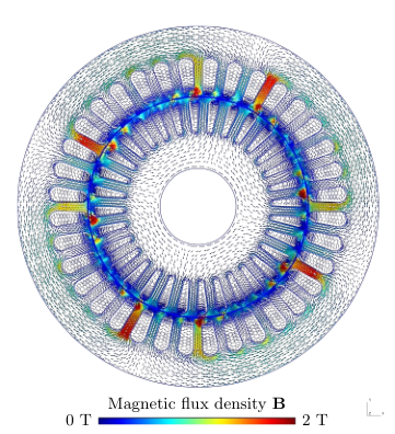
We will now illustrate the performance of our new Parareal algorithm (16)-(17) for the semi-discrete eddy current problem (49)-(50), supplied with a three-phase PWM voltage source. As a concrete example we consider a four-pole squirrel-cage induction motor, illustrated in Figure 6, and carry out the computations under no-load operation condition. The simulation of the 2D machine model was performed using the GetDP library [18] using degrees of freedom. The machine is supplied with a three-phase PWM voltage source of kHz, which corresponds to pulses on the time interval s, and is practically relevant for numerous applications in electrical engineering. For and , the excitation (in V) with pulses is given by
| (51) |
where denotes one of the three phases and
| (52) |
is determined by the bipolar trailing-edge modulation using a sawtooth carrier [35].
We consider s to be the electric period, which corresponds to a frequency of Hz. As an example of the voltage source, a PWM signal of kHz (corresponding to pulses on s) is shown in Figure 7.
An initial ramp-up of the applied voltage was used for reducing the transient behavior of the motor, as it was proposed by the original authors of the model [19]. Phase 1 of the three-phase sinusoidal voltage source of Hz is shown in Figure 7. This waveform will be used as an input for the reduced coarse problem within our new Parareal method.
The current waveforms, obtained by solving the DAE (49) excited by the PWM signal of kHz are shown in Figure 8.
The waveform has multiharmonic characteristics: one observes three different time scales: the underlying sinusoidal excitation (50 Hz), an additional sinusoidal behavior due to ‘slotting’ of the machine and finally the small high-frequency oscillations (‘ripples’) in the current waveforms due to the PWM excitations ( kHz). The consideration of all those frequencies may be for example important if an engineer is concerned with the acoustic design of the machine.
6.2 Application of the new Parareal algorithm
The new Parareal algorithm (16)-(17) was implemented in GNU Octave [9] and uses OpenMP parallelized calls of GetDP. It was executed on an Intel Xeon cluster with GHz cores and 1TB DDR3 memory.
The reduced coarse propagator solves (49)-(50) with the input three-phase voltage
| (53) |
for shown in Figure 9.
The fine solver uses the original PWM input , from (51). Both propagators solve the IVP using the Backward Euler method with the time step sizes s and s for the coarse and the fine problem, respectively. We have used cores within the new Parareal simulation, and for comparison we also simulated the machine with the original Parareal algorithm (7)-(8). In the original Parareal algorithm both coarse and fine problems have the same PWM voltage input and we use the same time step sizes and defined above.
In order to evaluate the convergence of the original and the new Parareal algorithms, we used the error norm from [20, Chapter II.4], i.e., the vector is considered close to if
| (54) |
where are prescribed absolute and relative tolerances. The error norm (54) is applied to each jump at the synchronization points. The Parareal iteration is terminated if the mismatch of the biggest jump, measured by (54), is below .
The numerical results in Figure 10 show that the new Parareal algorithm with well-chosen reduced coarse input works very well in practice: at each iteration, it is about one order of magnitude more accurate, and also needs in this example 25% less iterations than the original Parareal algorithm to converge to the desired tolerance, capturing well all relevant frequencies of the multiharmonic solution.
7 Conclusions
In this paper we proposed a new Parareal algorithm for problems which involve discontinuous inputs. Our new Parareal algorithm uses a smooth part of the source representing reduced dynamics for the coarse propagator, which is suitable for coarse discretization in time. We analyzed the new Parareal algorithm and derived precise error estimates, which show that order reduction is possible if the coarse model is not good enough. In particular, if the chosen non-smooth part of the input belongs to with , and a time integrator of order is used as the coarse propagator for the reduced problem, we proved that the order reduction can be at most . However, if the corresponding input with reduced dynamics is a good approximation to the original (discontinuous) input, i.e., they are close in the sense of the norm, then the new Parareal algorithm with a coarse propagator using large time steps reaches the same order as the original Parareal algorithm that would need a coarse propagator with very small time steps. We illustrated the accuracy of our estimates with numerical experiments on an RL-circuit model with PWM signal as input, and we also tested the new Parareal algorithm on an eddy current problem, describing the operation of an induction machine. The new Parareal algorithm is about an order of magnitude more accurate in each iteration than the original one, and reaches a prescribed tolerance in less iterations in the eddy current example.
References
- [1] M. Astorino, F. Chouly, and A. Quarteroni, Multiscale coupling of finite element and lattice Boltzmann methods for time dependent problems, tech. report, http://hal. archives-ouvertes. fr/hal-00746942, 2012.
- [2] L. Baffico, S. Bernard, Y. Maday, G. Turinici, and G. Zérah, Parallel-in-time molecular-dynamics simulations, Phys. Rev. E, 66 (2002), p. 057701, 10.1103/PhysRevE.66.057701.
- [3] G. Bal, Parallelization in time of (stochastic) ordinary differential equations, Math. Meth. Anal. Num.(submitted), (2003).
- [4] G. Barenblatt and A. J. Chorin, New perspectives in turbulence: Scaling laws, asymptotics, and intermittency, SIAM review, 40 (1998), pp. 265–291.
- [5] Y. Boubendir, X. Antoine, and C. Geuzaine, A quasi-optimal non-overlapping domain decomposition algorithm for the Helmholtz equation, Journal of Computational Physics, 231 (2012), pp. 262–280.
- [6] F. Chen, J. S. Hesthaven, and X. Zhu, On the use of reduced basis methods to accelerate and stabilize the parareal method, in Reduced Order Methods for Modeling and Computational Reduction, Springer, 2014, pp. 187–214.
- [7] F. Chouly and A. Lozinski, Parareal multi-model numerical zoom for parabolic multiscale problems, Comptes Rendus Mathematique, 352 (2014), pp. 535–540.
- [8] G. Dahlquist and Å. Björck, Numerical methods in scientific computing, volume I, SIAM, 2007.
- [9] J. W. Eaton, D. Bateman, S. Hauberg, and R. Wehbring, The GNU Octave 4.0 Reference Manual 1/2: Free Your Numbers, Samurai Media Limited, Oct. 2015, http://www.gnu.org/software/octave/doc/interpreter.
- [10] S. Engblom, Parallel in Time Simulation of Multiscale Stochastic Chemical Kinetics, Multiscale Modeling & Simulation, 8 (2009), pp. 46–68, https://doi.org/10.1137/080733723.
- [11] M. V. Ferreira da Luz, P. Dular, N. Sadowski, C. Geuzaine, and J. P. A. Bastos, Analysis of a permanent magnet generator with dual formulations using periodicity conditions and moving band, IEEE Trans. Magn., 38 (2002), pp. 961–964, https://doi.org/10.1109/20.996247.
- [12] A. F. Filippov, Differential equations with discontinuous righthand sides: control systems, vol. 18, Springer Science & Business Media, 2013.
- [13] P. F. Fischer, F. Hecht, and Y. Maday, A parareal in time semi-implicit approximation of the Navier-Stokes equations, in Domain Decomposition Methods in Science and Engineering, R. Kornhuber and et al., eds., vol. 40 of Lecture Notes in Computational Science and Engineering, Berlin, 2005, Springer, pp. 433–440, https://doi.org/10.1007/3-540-26825-1_44.
- [14] M. J. Gander, Optimized Schwarz methods, SIAM Journal on Numerical Analysis, 44 (2006), pp. 699–731.
- [15] M. J. Gander, 50 years of time parallel time integration, in Multiple Shooting and Time Domain Decomposition Methods, Springer, 2015, pp. 69–113.
- [16] M. J. Gander and E. Hairer, Nonlinear convergence analysis for the Parareal algorithm, Springer, 2008.
- [17] M. J. Gander and S. Vandewalle, Analysis of the Parareal time-parallel time-integration method, SIAM Journal on Scientific Computing, 29 (2007), pp. 556–578.
- [18] C. Geuzaine, GetDP: a general finite-element solver for the de Rham complex, PAMM, 7 (2007), pp. 1010603–1010604, https://doi.org/10.1002/pamm.200700750.
- [19] J. Gyselinck, L. Vandevelde, and J. Melkebeek, Multi-slice FE modeling of electrical machines with skewed slots-the skew discretization error, IEEE Trans. Magn., 37 (2001), pp. 3233–3237, https://doi.org/10.1109/20.952584.
- [20] E. Hairer, S. Norsett, and G. Wanner, Solving Ordinary Differential Equations I, Nonstiff problems/E. Hairer, SP Norsett, G. Wanner, with 135 Figures, Vol.: 1, 2Ed. Springer-Verlag, 2000, 2000.
- [21] T. Haut and B. Wingate, An asymptotic parallel-in-time method for highly oscillatory PDEs, SIAM Journal on Scientific Computing, 36 (2014), pp. A693–A713.
- [22] L. He, The reduced basis technique as a coarse solver for parareal in time simulations, Journal of Computational Mathematics, 28 (2010), pp. 676–692.
- [23] J. D. Jackson, Classical Electrodynamics, Wiley and Sons, New York, 3rd ed., 1998.
- [24] J.-L. Lions, Y. Maday, and G. Turinici, A parareal in time discretization of PDEs, Comptes Rendus de l’Académie des Sciences – Series I – Mathematics, 332 (2001), pp. 661–668, https://doi.org/10.1016/S0764-4442(00)01793-6.
- [25] J. Liu and Y.-L. Jiang, A parareal waveform relaxation algorithm for semi-linear parabolic partial differential equations, Journal of Computational and Applied Mathematics, 236 (2012), pp. 4245–4263, https://doi.org/10.1016/j.cam.2012.05.014.
- [26] Y. Maday, The Parareal in time algorithm, in Substructuring Techniques and Domain Decomposition Methods, Saxe-Coburg Publications, 2008.
- [27] Y. Maday, J. Salomon, and G. Turinici, Monotonic parareal control for quantum systems, SIAM Journal on Numerical Analysis, 45 (2007), pp. 2468–2482, https://doi.org/10.1137/050647086.
- [28] Y. Maday and G. Turinici, Parallel in time algorithms for quantum control: Parareal time discretization scheme, Int. J. Quant. Chem., 93 (2003), pp. 223–228, https://doi.org/10.1002/qua.10554.
- [29] A. S. Nielsen, Feasibility study of the parareal algorithm, 2012.
- [30] A. Quarteroni and A. Valli, Domain Decomposition Methods for Partial Differential Equations, Numerical Mathematics and Scientific Computation, Oxford University Press, Oxford, 1999.
- [31] K. Schmidt, O. Sterz, and R. Hiptmair, Estimating the eddy-current modeling error, IEEE Trans. Magn., 44 (2008), pp. 686–689, https://doi.org/10.1109/TMAG.2008.915834.
- [32] S. Schöps, H. De Gersem, and T. Weiland, Winding functions in transient magnetoquasistatic field-circuit coupled simulations, COMPEL, 32 (2013), pp. 2063–2083, https://doi.org/10.1108/COMPEL-01-2013-0004.
- [33] S. Schöps, I. Niyonzima, and M. Clemens, Parallel-in-time simulation of eddy current problems using parareal, IEEE Trans. Magn., 54 (2018), https://doi.org/10.1109/TMAG.2017.276309, https://arxiv.org/abs/1706.05750.
- [34] G. Staff, Convergence and Stability of the Parareal Algorithm, master’s thesis, Norwegian University of Science and Technology, Norway, 2003.
- [35] J. Sun, Pulse-Width Modulation, Springer-Verlag London, London, 2012, pp. 25–61, https://doi.org/10.1007/978-1-4471-2885-4.
- [36] A. Toselli and O. B. Widlund, Domain decomposition methods: algorithms and theory, vol. 34, Springer, 2005.
- [37] J. M. F. Trindade and J. C. F. Pereira, Parallel-in-time simulation of the unsteady Navier-Stokes equations for incompressible flow, International Journal for Numerical Methods in Fluids, 45 (2004), pp. 1123–1136, https://doi.org/10.1002/fld.732.