跳到论文正文
W Papers独立论文阅读器 arXiv:1803.05309 论文正文 计算阅读时间 · 0%
引用这篇论文根据当前论文元数据生成,正式投稿前建议核对。


License: arXiv.org perpetual non-exclusive license
arXiv:1803.05309v2 [math.NA] 03 Jul 2018

Direct sampling method for imaging small anomalies: real-data experiments

Won-Kwang Park Email: parkwk@kookmin.ac.kr Address: Department of Information Security, Cryptology, and Mathematics, Kookmin University, Seoul, 02707, Korea. Corresponding author: First and corresponding author    Kwang-Jae Lee Email: reolee0122@etri.re.kr    Seong-Ho Son Email: shs@etri.re.kr Address: Radio Environment & Monitoring Research Group, Electronics and Telecommunications Research Institute, Daejeon, 34129, Korea Corresponding author: Co-corresponding author
Abstract

In this paper, a direct sampling method (DSM) is designed for a real-time detection of small anomalies from scattering parameters measured by a small number of dipole antennas. Applicability of the DSM is theoretically demonstrated by proving that its indicator function can be represented in terms of an infinite series of Bessel functions of integer order, Hankel function of order zero, and the antenna configurations. Experiments using real-data then demonstrate both the effectiveness and limitations of this method.

Keywords: 
Direct sampling method , scattering parameter , Bessel and Hankel functions , Real-data experiments

1 Introduction

Several studies have revealed that the direct sampling method (DSM) is a fast, stable, and effective imaging technique in inverse scattering problems. It has been investigated for imaging small two-dimensional anomalies [1, 2, 3, 4] and retrieving three-dimensional objects [5] for diffusive [6] and electrical impedance [7] tomography applications and for source detection in stratified ocean waveguides [8]. As we have previously observed, DSM only requires one or at most a few incident fields, rather than additional operations, such as singular value decomposition [9, 10] or solving ill-posed integral equations [11] or adjoint problems [12, 13].

Recent study [14] has shown that the DSM is an effective technique for microwave imaging; however, their simulations differ in crucial ways from real-world scenarios: for example, it is difficult to measure scattering parameters when the transmitting and receiving antennas are in the same location. An extended study that considered a more realistic scenario is required and experiments using real-data should be conducted to show that this method could feasibly be used for real-world applications. Therefore, an appropriate DSM is designed herein, and its mathematical structure is analyzed to demonstrate its real-world applicability.

This study is an extension of a previous study [14] on analyzing the DSM’s structure to a real-world application. Herein, the DSM is designed to handle a real-world problem, and the mathematical structure of its indicator function is analyzed by expressing it in terms of an infinite series of Bessel functions of integer order. Finally, the imaging performance of designed DSM and related factors are discussed.

This paper is organized as follows. Section 2 briefly discusses the scattering parameters in the presence of a set of anomalies and designing of an indicator function of DSM. Section 3 investigates the structure of this indicator function by expressing it in terms of an infinite series of Bessel functions of the first kind of integer order, Hankel function of order zero, and the antenna configuration. With this, we discuss the factors that influence its imaging performance. Section 4 contains experimental results using real-data for multiple anomalies for supporting theoretical result. Section 5 presents our conclusions and future works.

2 Scattering parameters and direct sampling method

This section briefly introduces the scattering parameters and discusses the design of a DSM indicator function. Here, we assume that multiple small anomalies Dm\mathrm{D}_{m} with smooth boundaries ∂Dm\partial\mathrm{D}_{m}, m=1,2,⋯,Mm=1,2,\cdots,M, exist in a homogeneous background medium. For simplicity, the Dm\mathrm{D}_{m} are assumed to be small balls of radius ρm\rho_{m} located at 𝐫m\mathbf{r}_{m} and denote the collection of all Dm\mathrm{D}_{m} by D\mathrm{D}. All the anomalies are contained in a homogeneous domain Ω\Omega and are surrounded by NN different dipole antennas 𝐚n\mathbf{a}_{n}, n=1,2,⋯,Nn=1,2,\cdots,N, located on a circle of radius RR. We denote the set of all antennas by A\mathrm{A}.

Throughout this study, the materials and anomalies are characterized by their dielectric permittivity and electrical conductivity at a given angular frequency ω=2​π​f\omega=2\pi f. The magnetic permeability is set to be a constant μ⁡(𝐫)≡μ=4⋅10−7​π\mu(\mathbf{r})\equiv\mu=4\cdot 10^{-7}\pi for 𝐫∈Ω\mathbf{r}\in\Omega and the permittivity (conductivity) of the background and Dm\mathrm{D}_{m} are denoted by εb\varepsilon_{\mathrm{b}} (σb\sigma_{\mathrm{b}}) and εm\varepsilon_{m} (σm\sigma_{m}), respectively. In addition, the wavenumber kk is given by ω2​μb​(εb+i​σb/ω)\omega^{2}\mu_{\mathrm{b}}(\varepsilon_{\mathrm{b}}+i\sigma_{\mathrm{b}}/\omega).

The scattering parameters (S−S-parameters) S⁡(n,n′)\mathrm{S}(n,n^{\prime}) are defined as the ratios of the output voltages (or reflected waves) at the 𝐚n\mathbf{a}_{n} to the input voltages (or incident waves) at 𝐚n′\mathbf{a}_{n^{\prime}}. The measured data is the scattered field Sscat​(n,n′)\mathrm{S}_{\mathrm{scat}}(n,n^{\prime}), which is obtained by subtracting the S−S-parameters with and without anomalies, respectively. Then, based on [15], Sscat​(n,n′)\mathrm{S}_{\mathrm{scat}}(n,n^{\prime}) is given by

Sscat​(n,n′)=i​k24​ω​μb​∫Ω(ε⁡(𝐫)−εbεb+i​σ⁡(𝐫)−σbω​σb)​𝐄inc​(𝐚n′,𝐫)⋅𝐄tot​(𝐫,𝐚n)​𝑑𝐫,\mathrm{S}_{\mathrm{scat}}(n,n^{\prime})=\frac{ik^{2}}{4\omega\mu_{\mathrm{b}}}\int_{\Omega}\left(\frac{\varepsilon(\mathbf{r})-\varepsilon_{\mathrm{b}}}{\varepsilon_{\mathrm{b}}}+i\frac{\sigma(\mathbf{r})-\sigma_{\mathrm{b}}}{\omega\sigma_{\mathrm{b}}}\right)\mathbf{E}_{\mathrm{inc}}(\mathbf{a}_{n^{\prime}},\mathbf{r})\cdot\mathbf{E}_{\mathrm{tot}}(\mathbf{r},\mathbf{a}_{n})d\mathbf{r}, (1)

where 𝐄inc​(𝐚n′,𝐫)\mathbf{E}_{\mathrm{inc}}(\mathbf{a}_{n^{\prime}},\mathbf{r}) is the incident electric field in a homogeneous medium due to the point current density at 𝐚n′\mathbf{a}_{n^{\prime}}, which satisfies

OPEN∇×𝐄inc​(𝐚n′,𝐫)=−i​ω​μ​𝐇​(𝐚n′,𝐫))and∇×𝐇⁡(𝐚n′,𝐫)=(σb+i​ω​εb)​𝐄inc​(𝐚n′,𝐫),\nabla\times\mathbf{E}_{\mathrm{inc}}(\mathbf{a}_{n^{\prime}},\mathbf{r})=-i\omega\mu\mathbf{H}(\mathbf{a}_{n^{\prime}},\mathbf{r}))\quad\mbox{and}\quad\nabla\times\mathbf{H}(\mathbf{a}_{n^{\prime}},\mathbf{r})=(\sigma_{\mathrm{b}}+i\omega\varepsilon_{\mathrm{b}})\mathbf{E}_{\mbox{\tiny inc}}(\mathbf{a}_{n^{\prime}},\mathbf{r}),

and 𝐄tot​(𝐫,𝐚n)\mathbf{E}_{\mathrm{tot}}(\mathbf{r},\mathbf{a}_{n}) be the total field owing to the presence of the anomalies D\mathrm{D} measured at 𝐚n\mathbf{a}_{n}, which satisfies

∇×𝐄tot​(𝐫,𝐚n)=−i​ω​μ​𝐇​(𝐫,𝐚n)and∇×𝐇⁡(𝐫,𝐚n)=(σ⁡(𝐫)+i​ω​ε​(𝐫))​𝐄tot​(𝐫,𝐚n),\nabla\times\mathbf{E}_{\mathrm{tot}}(\mathbf{r},\mathbf{a}_{n})=-i\omega\mu\mathbf{H}(\mathbf{r},\mathbf{a}_{n})\quad\mbox{and}\quad\nabla\times\mathbf{H}(\mathbf{r},\mathbf{a}_{n})=(\sigma(\mathbf{r})+i\omega\varepsilon(\mathbf{r}))\mathbf{E}_{\mathrm{tot}}(\mathbf{r},\mathbf{a}_{n}),

with transmission conditions at the boundaries ∂D\partial\mathrm{D}. Here, we assume a time-harmonic dependence ei​ω​te^{i\omega t}, and 𝐇\mathbf{H} denotes the magnetic field.

It is worth noting that, in general real-world experiments, it is impossible to measure Sscat​(n,n′)\mathrm{S}_{\mathrm{scat}}(n,n^{\prime}) when n=n′n=n^{\prime} because antenna 𝐚n′\mathbf{a}_{n^{\prime}} is used for signal transmission and the remaining N−1N-1 antennas 𝐚n\mathbf{a}_{n}, n=1,2,⋯,Nn=1,2,\cdots,N with n≠n′n\neq n^{\prime} are used for signal reception. Thus, the indicator function introduced in [1, 2, 4, 14] cannot be applied for imaging of D\mathrm{D}.

Motivated by the above, we design an indicator function of DSM for imaging D\mathrm{D} by finding their positions 𝐫m\mathbf{r}_{m} based on the measured data Sscat​(n,n′)\mathrm{S}_{\mathrm{scat}}(n,n^{\prime}) for fixed n′n^{\prime}. Since the anomalies are assumed to be small, applying the Born approximation to (1) yields

Sscat​(n,n′)=i​k24​ω​μb​∑m=1Mρm3​χ​(𝐫m)​𝐄inc​(𝐚n′,𝐫m)⋅𝐄inc​(𝐫m,𝐚n)+o⁡(ρm3),χ⁡(𝐫m)=εm−εbεb+i​σm−σbω​σb.\mathrm{S}_{\mathrm{scat}}(n,n^{\prime})=\frac{ik^{2}}{4\omega\mu_{\mathrm{b}}}\sum_{m=1}^{M}\rho_{m}^{3}\chi(\mathbf{r}_{m})\mathbf{E}_{\mathrm{inc}}(\mathbf{a}_{n^{\prime}},\mathbf{r}_{m})\cdot\mathbf{E}_{\mathrm{inc}}(\mathbf{r}_{m},\mathbf{a}_{n})+o(\rho_{m}^{3}),\quad\chi(\mathbf{r}_{m})=\frac{\varepsilon_{m}-\varepsilon_{\mathrm{b}}}{\varepsilon_{\mathrm{b}}}+i\frac{\sigma_{m}-\sigma_{\mathrm{b}}}{\omega\sigma_{\mathrm{b}}}. (2)

Based on this representation, we introduce the indicator function of DSM as follows. For 𝐫∈Ω\mathbf{r}\in\Omega,

𝔉DSM​(𝐫,n′)=|⟨Sscat​(n,n′),𝐄inc​(𝐫,𝐚n)⟩L2​(A)|‖Sscat​(n,n′)‖L2​(A)​‖𝐄inc​(𝐫,𝐚n)‖L2​(A),\mathfrak{F}_{\mathrm{DSM}}(\mathbf{r},n^{\prime})=\frac{|\langle\mathrm{S}_{\mathrm{scat}}(n,n^{\prime}),\mathbf{E}_{\mathrm{inc}}(\mathbf{r},\mathbf{a}_{n})\rangle_{L^{2}(\mathrm{A})}|}{||\mathrm{S}_{\mathrm{scat}}(n,n^{\prime})||_{L^{2}(\mathrm{A})}||\mathbf{E}_{\mathrm{inc}}(\mathbf{r},\mathbf{a}_{n})||_{L^{2}(\mathrm{A})}}, (3)

where

⟨𝐟⁡(𝐚n),𝐠⁡(𝐚n)⟩L2​(A)=∑n=1,n≠n′N𝐟⁡(𝐚n)​𝐠⁡(𝐚n)¯and‖𝐟⁡(𝐚n)‖L2​(A)=(⟨𝐟⁡(𝐚n),𝐟⁡(𝐚n)⟩L2​(A))1/2.\langle\mathbf{f}(\mathbf{a}_{n}),\mathbf{g}(\mathbf{a}_{n})\rangle_{L^{2}(\mathrm{A})}=\sum_{n=1,n\neq n^{\prime}}^{N}\mathbf{f}(\mathbf{a}_{n})\overline{\mathbf{g}(\mathbf{a}_{n})}\quad\mbox{and}\quad||\mathbf{f}(\mathbf{a}_{n})||_{L^{2}(\mathrm{A})}=(\langle\mathbf{f}(\mathbf{a}_{n}),\mathbf{f}(\mathbf{a}_{n})\rangle_{L^{2}(\mathrm{A})})^{1/2}.

Notice that the definition of 𝔉DSM​(𝐫,n′)\mathfrak{F}_{\mathrm{DSM}}(\mathbf{r},n^{\prime}) is different from the traditional indicator function of DSM. Nevertheless, the maps of 𝔉DSM​(𝐫,n′)\mathfrak{F}_{\mathrm{DSM}}(\mathbf{r},n^{\prime}) shown later contain large peaks at 𝐫≈𝐫m\mathbf{r}\approx\mathbf{r}_{m} and small values at 𝐫≠𝐫m\mathbf{r}\neq\mathbf{r}_{m}; therefore, the locations of the Dm\mathrm{D}_{m} can be identified via this DSM.

3 Theoretical result

This section investigates the mathematical structure of 𝔉DSM​(𝐫,n′)\mathfrak{F}_{\mathrm{DSM}}(\mathbf{r},n^{\prime}) by proving it can be written in terms of Bessel functions of integer order. It should be noted that, since the omnidirectional antennas are arranged perpendicular to the z−z-axis, the mathematical treatment of time-harmonic electromagnetic waves scattered from thin, infinitely-long cylindrical obstacles, (e.g., [10]) indicating that this problem can be regarded as two-dimensional, and the incident field can be expressed as 𝐄inc(𝐫,𝐚n)=−iH0(1)(k|𝐫−𝐚n|)/4\mathbf{E}_{\mathrm{inc}}(\mathbf{r},\mathbf{a}_{n})=-iH_{0}^{(1)}(k|\mathbf{r}-\mathbf{a}_{n}|)/4, where H0(1)H_{0}^{(1)} is the Hankel function of order zero. Based on this, the following result can be derived.

Theorem 3.1 (Mathematical structure of the indicator function).

Assume that the total number of antennas, NN, is small. Let |𝐚n|=R|\mathbf{a}_{n}|=R, 𝛉n:=𝐚n/|𝐚n|=(cos⁡θn,sin⁡θn)\boldsymbol{\theta}_{n}:=\mathbf{a}_{n}/|\mathbf{a}_{n}|=(\cos\theta_{n},\sin\theta_{n}), and 𝐫−𝐫m=|𝐫−𝐫m|(cosϕmsinϕm)\mathbf{r}-\mathbf{r}_{m}=|\mathbf{r}-\mathbf{r}_{m}|(\cos\phi_{m}\sin\phi_{m}). If k​|𝐫−𝐚n|≫0.25k|\mathbf{r}-\mathbf{a}_{n}|\gg 0.25 for 𝐫∈Ω\mathbf{r}\in\Omega, then 𝔉DSM​(𝐫,n′)\mathfrak{F}_{\mathrm{DSM}}(\mathbf{r},n^{\prime}) can be represented as follows:

𝔉DSM​(𝐫,n′)=|Φ⁡(𝐫)|max𝐫∈Ω⁡|Φ⁡(𝐫)|,\mathfrak{F}_{\mathrm{DSM}}(\mathbf{r},n^{\prime})=\frac{|\Phi(\mathbf{r})|}{\displaystyle\max_{\mathbf{r}\in\Omega}|\Phi(\mathbf{r})|}, (4)

where

Φ⁡(𝐫)≈∑m=1Mρm3​χ​(𝐫m)​H0(1)​(k​|𝐫m−𝐚n′|)​(J0​(k​|𝐫−𝐫m|)+1N−1​∑n=1,n≠n′N∑s∈ℤ¯0is​Js​(k​|𝐫−𝐫m|)​ei​s​(θn−ϕm)).\Phi(\mathbf{r})\approx\sum_{m=1}^{M}\rho_{m}^{3}\chi(\mathbf{r}_{m})H_{0}^{(1)}(k|\mathbf{r}_{m}-\mathbf{a}_{n^{\prime}}|)\left(J_{0}(k|\mathbf{r}-\mathbf{r}_{m}|)+\frac{1}{N-1}\sum_{n=1,n\neq n^{\prime}}^{N}\sum_{s\in\overline{\mathbb{Z}}_{0}}i^{s}J_{s}(k|\mathbf{r}-\mathbf{r}_{m}|)e^{is(\theta_{n}-\phi_{m})}\right).

Here, ℤ¯0=ℤ∪{−∞,+∞}\{0}\overline{\mathbb{Z}}_{0}=\mathbb{Z}\cup\left\{-\infty,+\infty\right\}\backslash\left\{0\right\} and ℤ\mathbb{Z} denotes the set of integer number.

Proof.

From (2), we can observe that

⟨Sscat​(n,n′),𝐄inc​(𝐫,𝐚n)⟩L2​(A)=i​k24​ω​μb​∑n=1,n≠n′N∑m=1Mρm3​χ​(𝐫m)​𝐄inc​(𝐚n′,𝐫m)⋅𝐄inc​(𝐫m,𝐚n)​𝐄inc​(𝐫,𝐚n)¯+o⁡(ρm3)≈−k2256​ω​μb∑m=1Mρm3χ(𝐫m)H0(1)(k|𝐫m−𝐚n′|)(∑n=1,n≠n′NH0(1)(k|𝐫m−𝐚n|)H0(1)​(k​|𝐫−𝐚n|)¯).\langle\mathrm{S}_{\mathrm{scat}}(n,n^{\prime}),\mathbf{E}_{\mathrm{inc}}(\mathbf{r},\mathbf{a}_{n})\rangle_{L^{2}(\mathrm{A})}=\frac{ik^{2}}{4\omega\mu_{\mathrm{b}}}\sum_{n=1,n\neq n^{\prime}}^{N}\sum_{m=1}^{M}\rho_{m}^{3}\chi(\mathbf{r}_{m})\mathbf{E}_{\mathrm{inc}}(\mathbf{a}_{n^{\prime}},\mathbf{r}_{m})\cdot\mathbf{E}_{\mathrm{inc}}(\mathbf{r}_{m},\mathbf{a}_{n})\overline{\mathbf{E}_{\mathrm{inc}}(\mathbf{r},\mathbf{a}_{n})}+o(\rho_{m}^{3})\\ \approx-\frac{k^{2}}{256\omega\mu_{\mathrm{b}}}\sum_{m=1}^{M}\rho_{m}^{3}\chi(\mathbf{r}_{m})H_{0}^{(1)}(k|\mathbf{r}_{m}-\mathbf{a}_{n^{\prime}}|)\left(\sum_{n=1,n\neq n^{\prime}}^{N}H_{0}^{(1)}(k|\mathbf{r}_{m}-\mathbf{a}_{n}|)\overline{H_{0}^{(1)}(k|\mathbf{r}-\mathbf{a}_{n}|)}\right). (5)

Since 𝐫m∈Ω\mathbf{r}_{m}\in\Omega and k​|𝐫−𝐚n|≫0.25k|\mathbf{r}-\mathbf{a}_{n}|\gg 0.25 for all 𝐫∈Ω\mathbf{r}\in\Omega, substituting the Hankel function’s asymptotic form

H0(1)(k|𝐫−𝐚n|)=1+i4​k​πei​k​RRe−ik𝜽n⋅𝐫+o(1k​R)H_{0}^{(1)}(k|\mathbf{r}-\mathbf{a}_{n}|)=\frac{1+i}{4\sqrt{k\pi}}\frac{e^{ikR}}{\sqrt{R}}e^{-ik\boldsymbol{\theta}_{n}\cdot\mathbf{r}}+o\left(\frac{1}{\sqrt{kR}}\right)

yields

∑n=1,n≠n′NH0(1)​(k​|𝐫−𝐚n|)​H0(1)​(k​|𝐫−𝐚n|)¯=∑n=1,n≠n′N18​k​π​Re−ik𝜽n⋅𝐫mei​k​𝜽n⋅𝐫+o(1k​R)≈18​k​π​R​∑n=1Nei​k​𝜽n⋅(𝐫−𝐫m)−18​k​π​R​ei​k​𝜽n′⋅(𝐫−𝐫m).\displaystyle\begin{aligned} \sum_{n=1,n\neq n^{\prime}}^{N}H_{0}^{(1)}(k|\mathbf{r}-\mathbf{a}_{n}|)\overline{H_{0}^{(1)}(k|\mathbf{r}-\mathbf{a}_{n}|)}&=\sum_{n=1,n\neq n^{\prime}}^{N}\frac{1}{8k\pi R}e^{-ik\boldsymbol{\theta}_{n}\cdot\mathbf{r}_{m}}e^{ik\boldsymbol{\theta}_{n}\cdot\mathbf{r}}+o\left(\frac{1}{\sqrt{kR}}\right)\\ &\approx\frac{1}{8k\pi R}\sum_{n=1}^{N}e^{ik\boldsymbol{\theta}_{n}\cdot(\mathbf{r}-\mathbf{r}_{m})}-\frac{1}{8k\pi R}e^{ik\boldsymbol{\theta}_{n^{\prime}}\cdot(\mathbf{r}-\mathbf{r}_{m})}.\end{aligned} (6)

Since 𝜽n⋅(𝐫−𝐫m)=|𝐫−𝐫m|​cos⁡(θn−ϕm)\boldsymbol{\theta}_{n}\cdot(\mathbf{r}-\mathbf{r}_{m})=|\mathbf{r}-\mathbf{r}_{m}|\cos(\theta_{n}-\phi_{m}) and the Jacobi-Anger expansion

ei​x​cos⁡θ=J0​(x)+∑s∈ℤ¯0is​Js​(x)​ei​s​θe^{ix\cos\theta}=J_{0}(x)+\sum_{s\in\overline{\mathbb{Z}}_{0}}i^{s}J_{s}(x)e^{is\theta}

holds uniformly, we can obtain

∑n=1Nei​k​𝜽n⋅(𝐫−𝐫m)=∑n=1Nei​k​|𝐫−𝐫m|​cos⁡(θn−ϕm)=∑n=1N(J0​(k​|𝐫−𝐫m|)+∑s∈ℤ¯0is​Js​(k​|𝐫−𝐫m|)​ei​s​(θn−ϕm))=N​J0​(k​|𝐫−𝐫m|)+∑n=1N∑s∈ℤ¯0is​Js​(k​|𝐫−𝐫m|)​ei​s​(θn−ϕm)\displaystyle\begin{aligned} \sum_{n=1}^{N}e^{ik\boldsymbol{\theta}_{n}\cdot(\mathbf{r}-\mathbf{r}_{m})}&=\sum_{n=1}^{N}e^{ik|\mathbf{r}-\mathbf{r}_{m}|\cos(\theta_{n}-\phi_{m})}=\sum_{n=1}^{N}\left(J_{0}(k|\mathbf{r}-\mathbf{r}_{m}|)+\sum_{s\in\overline{\mathbb{Z}}_{0}}i^{s}J_{s}(k|\mathbf{r}-\mathbf{r}_{m}|)e^{is(\theta_{n}-\phi_{m})}\right)\\ &=NJ_{0}(k|\mathbf{r}-\mathbf{r}_{m}|)+\sum_{n=1}^{N}\sum_{s\in\overline{\mathbb{Z}}_{0}}i^{s}J_{s}(k|\mathbf{r}-\mathbf{r}_{m}|)e^{is(\theta_{n}-\phi_{m})}\end{aligned} (7)

and, similarly,

ei​k​𝜽n′⋅(𝐫−𝐫m)=J0​(k​|𝐫−𝐫m|)+∑s∈ℤ¯0is​Js​(k​|𝐫−𝐫m|)​ei​s​(θn′−ϕm).e^{ik\boldsymbol{\theta}_{n^{\prime}}\cdot(\mathbf{r}-\mathbf{r}_{m})}=J_{0}(k|\mathbf{r}-\mathbf{r}_{m}|)+\sum_{s\in\overline{\mathbb{Z}}_{0}}i^{s}J_{s}(k|\mathbf{r}-\mathbf{r}_{m}|)e^{is(\theta_{n}^{\prime}-\phi_{m})}. (8)

Combining (7) and (8), (6) can be rewritten as

∑n=1,n≠n′NH0(1)​(k​|𝐫−𝐚n|)​H0(1)​(k​|𝐫−𝐚n|)¯≈N−18​k​π​R​(J0​(k​|𝐫−𝐫m|)+1N−1​∑n=1,n≠n′N∑s∈ℤ¯0is​Js​(k​|𝐫−𝐫m|)​ei​s​(θn−ϕm)).\sum_{n=1,n\neq n^{\prime}}^{N}H_{0}^{(1)}(k|\mathbf{r}-\mathbf{a}_{n}|)\overline{H_{0}^{(1)}(k|\mathbf{r}-\mathbf{a}_{n}|)}\\ \approx\frac{N-1}{8k\pi R}\left(J_{0}(k|\mathbf{r}-\mathbf{r}_{m}|)+\frac{1}{N-1}\sum_{n=1,n\neq n^{\prime}}^{N}\sum_{s\in\overline{\mathbb{Z}}_{0}}i^{s}J_{s}(k|\mathbf{r}-\mathbf{r}_{m}|)e^{is(\theta_{n}-\phi_{m})}\right). (9)

Finally, substituting (9) into (5) leads us to

⟨Sscat(n,n′),𝐄inc(𝐫,𝐚n)⟩L2​(A)≈−(N−1)​k2048​R​ω​μb​π∑m=1Mρm3χ(𝐫m)H0(1)(k|𝐫m−𝐚n′|)×(J0​(k​|𝐫−𝐫m|)+1N−1​∑n=1,n≠n′N∑s∈ℤ¯0is​Js​(k​|𝐫−𝐫m|)​ei​s​(θn−ϕm)).\langle\mathrm{S}_{\mathrm{scat}}(n,n^{\prime}),\mathbf{E}_{\mathrm{inc}}(\mathbf{r},\mathbf{a}_{n})\rangle_{L^{2}(\mathrm{A})}\approx-\frac{(N-1)k}{2048R\omega\mu_{\mathrm{b}}\pi}\sum_{m=1}^{M}\rho_{m}^{3}\chi(\mathbf{r}_{m})H_{0}^{(1)}(k|\mathbf{r}_{m}-\mathbf{a}_{n^{\prime}}|)\\ \times\left(J_{0}(k|\mathbf{r}-\mathbf{r}_{m}|)+\frac{1}{N-1}\sum_{n=1,n\neq n^{\prime}}^{N}\sum_{s\in\overline{\mathbb{Z}}_{0}}i^{s}J_{s}(k|\mathbf{r}-\mathbf{r}_{m}|)e^{is(\theta_{n}-\phi_{m})}\right).

With this, applying Hölder’s inequality,

⟨Sscat​(n,n′),𝐄inc​(𝐫,𝐚n)⟩L2​(A)≤‖Sscat​(n,n′)‖L2​(A)​‖𝐄inc​(𝐫,𝐚n)‖L2​(A),\langle\mathrm{S}_{\mathrm{scat}}(n,n^{\prime}),\mathbf{E}_{\mathrm{inc}}(\mathbf{r},\mathbf{a}_{n})\rangle_{L^{2}(\mathrm{A})}\leq||\mathrm{S}_{\mathrm{scat}}(n,n^{\prime})||_{L^{2}(\mathrm{A})}||\mathbf{E}_{\mathrm{inc}}(\mathbf{r},\mathbf{a}_{n})||_{L^{2}(\mathrm{A})},

allows us to obtain (4), thereby completing the proof. ∎

Remark 3.1.

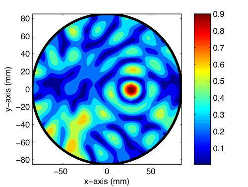
The indicator function structure (4) implies that the imaging performance is highly dependent on 1) the anomaly’s size, permittivity, and conductivity; 2) the antenna configuration (total number and arrangement); and 3) the distance between the transmitter 𝐚n′\mathbf{a}_{n^{\prime}} and anomaly Dm\mathrm{D}_{m}. Observations 1 and 2 have also been made by other studies [3, 4, 14], but observation 3 is also a significant factor that affects imaging performance in real-world applications, as shown below by the experimental results for Example 4.1.

4 Experimental results

To evaluate this theoretical result and demonstrate the effectiveness and limitations of the designed DSM, we now present the results of experiments with real-world data. For these experiments, we placed N=16N=16 dipole antennas in a circle of radius 0.090.09m as follows:

𝐚n=0.09​m​(cos⁡θn,sin⁡θn),withθn=3​π2−2​π​(n−1)N.\mathbf{a}_{n}=0.09\mbox{m}\left(\cos\theta_{n},\sin\theta_{n}\right),\quad\mbox{with}\quad\theta_{n}=\frac{3\pi}{2}-\frac{2\pi(n-1)}{N}.

The homogeneous background medium was filled with water, and its permittivity and conductivity were εb=78\varepsilon_{\mathrm{b}}=78 and σb=0.2\sigma_{\mathrm{b}}=0.2S/m, respectively. The imaging region Ω\Omega was set to be the interior of a circle of radius 0.0850.085m, centered at the origin. The S−S-parameters Sscat​(n,n′)\mathrm{S}_{\mathrm{scat}}(n,n^{\prime}) were measured using a microwave machine developed by the Electronics and Telecommunications Research Institute (ETRI), and the incident field data 𝐄inc​(𝐚n,𝐫)\mathbf{E}_{\mathrm{inc}}(\mathbf{a}_{n},\mathbf{r}) used to calculate the indicator function 𝔉DSM​(𝐫,n′)\mathfrak{F}_{\mathrm{DSM}}(\mathbf{r},n^{\prime}) via (3), were generated by CST STUDIO SUITE, as shown in Figure 1.

Refer to caption
Refer to caption
Refer to caption
Figure 1: Microwave machine (left) and real part of 𝐄inc​(𝐚n,𝐫)\mathbf{E}_{\mathrm{inc}}(\mathbf{a}_{n},\mathbf{r}) for n=4n=4 (center), and n=10n=10 (right).
Example 4.1.

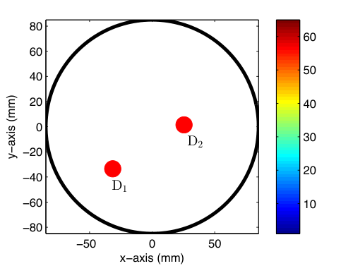
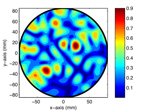
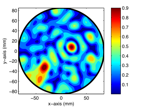
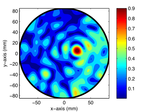
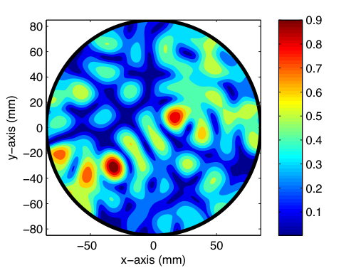
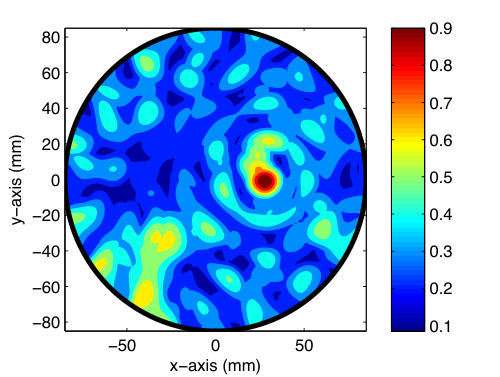
Here, we consider imaging two anomalies, D1\mathrm{D}_{1} and D2\mathrm{D}_{2}, both of diameter 0.00640.0064m. Maps of 𝔉DSM​(𝐫,n′)\mathfrak{F}_{\mathrm{DSM}}(\mathbf{r},n^{\prime}) for several different n′n^{\prime} are shown in Figure 2. Note that the locations of D1\mathrm{D}_{1} and D2\mathrm{D}_{2} can be identified, but some large artifacts also exist. It is also interesting to observe that D1\mathrm{D}_{1} cannot be identified when n′=9n^{\prime}=9 and n′=13n^{\prime}=13, i.e., when D1\mathrm{D}_{1} is not close enough to 𝐚n′\mathbf{a}_{n^{\prime}}. While D1\mathrm{D}_{1} can be located when n′=1n^{\prime}=1, n′=2n^{\prime}=2, and n′=5n^{\prime}=5, these provide the wrong location for D2\mathrm{D}_{2} because D2\mathrm{D}_{2} is not close enough to 𝐚n′\mathbf{a}_{n^{\prime}}.

Refer to caption
Refer to caption
Refer to caption
Refer to caption
Refer to caption
Refer to caption
Figure 2: True locations of the anomalies (top left) and maps of 𝔉DSM​(𝐫,n′)\mathfrak{F}_{\mathrm{DSM}}(\mathbf{r},n^{\prime}) for n′=1n^{\prime}=1 (top center), n′=5n^{\prime}=5 (top right), n′=9n^{\prime}=9 (bottom left), n′=13n^{\prime}=13 (bottom center), and n′=2n^{\prime}=2 (bottom right).
Example 4.2.

As observed in Example 4.1, the imaging performance is highly dependent on the location of the transducer 𝐚n′\mathbf{a}_{n^{\prime}}. To identify all the anomalies in Example 4.1, the following indicator function with multiple incident fields is adopted, introduced in [1, 2]. For each 𝐫∈Ω\mathbf{r}\in\Omega,

𝔉MDSM​(𝐫):=maxn′⁡{𝔉DSM​(𝐫,n′)}.\mathfrak{F}_{\mathrm{MDSM}}(\mathbf{r}):=\max_{n^{\prime}}\left\{\mathfrak{F}_{\mathrm{DSM}}(\mathbf{r},n^{\prime})\right\}.

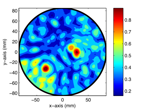
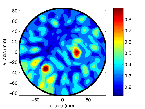
Figure 3 shows the maps of 𝔉MDSM​(𝐫)\mathfrak{F}_{\mathrm{MDSM}}(\mathbf{r}) for four (n′=1,5,9,13n^{\prime}=1,5,9,13), eight (n′=1,3,5,⋯,15n^{\prime}=1,3,5,\cdots,15), and sixteen (n′=1,2,3,⋯,16n^{\prime}=1,2,3,\cdots,16) different incident fields. These results indicate that the location of D1\mathrm{D}_{1} cannot be identified with a small number of incident directions but can be identified when sufficient incident directions are used. However, some artifacts still appear in the map; therefore, further improvement is still needed.
Refer to caption
Refer to caption
Refer to caption
Figure 3: Maps of 𝔉MDSM​(𝐫)\mathfrak{F}_{\mathrm{MDSM}}(\mathbf{r}) for four (left), eight (center), and sixteen (right) different incident fields.

5 Conclusions

An indicator function of DSM is designed for identifying small anomalies from scattering parameters measured by a small number of dipole antennas. The experimental results with real-data indicate that such small anomalies can be identified via this DSM with only one or at most a few incident fields, which means that it can be regarded as a fast imaging technique for real-world microwave imaging. Unfortunately, these results also include some artifacts, and the imaging performance depended significantly on the transmitter location. This has motivated us to develop an improved DSM, and this will be the subject of future study.

Acknowledgements

This research was supported by the Basic Science Research Program of the National Research Foundation of Korea (NRF) funded by the Ministry of Education (No. NRF-2017R1D1A1A09000547), the research program of Kookmin University in Korea, and Electronics and Telecommunications Research Institute (ETRI) grant funded by the Korean government (No. 18ZR1230).

References

  • [1] K. Ito, B. Jin, J. Zou, A direct sampling method to an inverse medium scattering problem, Inverse Problems 28 (2) (2012) 025003.
  • [2] J. Li, J. Zou, A direct sampling method for inverse scattering using far-field data, Inverse Probl. Imag. 7 (3) (2013) 757–775.
  • [3] S. Kang, M. Lambert, W.-K. Park, Direct sampling method for imaging small dielectric inhomogeneities: analysis and improvement, Inverse Problems accepted for publication.
  • [4] W.-K. Park, Detection of small inhomogeneities via direct sampling method in transverse electric polarization, Appl. Math. Lett. 79 (2018a) 169–175.
  • [5] K. Ito, B. Jin, J. Zou, A direct sampling method for inverse electromagnetic medium scattering, Inverse Problems 29 (9) (2013) 095018.
  • [6] Y. T. Chow, K. Ito, K. Liu, J. Zou, Direct sampling method for diffusive optical tomography, SIAM J. Sci. Comput. 37 (4) (2015) A1658–A1684.
  • [7] Y. T. Chow, K. Ito, J. Zou, A direct sampling method for electrical impedance tomography, Inverse Problems 30 (9) (2014) 095003.
  • [8] K. Liu, Y. Xu, J. Zou, A multilevel sampling method for detecting sources in a stratified ocean waveguide, J. Comput. Appl. Math. 309 (2017) 95–110.
  • [9] H. Ammari, E. Iakovleva, D. Lesselier, G. Perrusson, MUSIC type electromagnetic imaging of a collection of small three-dimensional inclusions, SIAM J. Sci. Comput. 29 (2) (2007) 674–709.
  • [10] W.-K. Park, H. P. Kim, K.-J. Lee, S.-H. Son, MUSIC algorithm for location searching of dielectric anomalies from S−{S}-parameters using microwave imaging, J. Comput. Phys. 348 (2017) 259–270.
  • [11] A. Kirsch, S. Ritter, A linear sampling method for inverse scattering from an open arc, Inverse Problems 16 (1) (2000) 89–105.
  • [12] F. L. Louër, M.-L. Rapún, Topological sensitivity for solving inverse multiple scattering problems in 3D electromagnetism. Part I: one step method, SIAM J. Imag. Sci. 10 (3) (2017) 1291–1321.
  • [13] A. A. Novotny, J. Sokolowski, Topological Derivatives in Shape Optimization, Interaction of Mechanics and Mathematics Series, Springer-Verlag, Berlin, Heidelberg, 2013.
  • [14] W.-K. Park, Direct sampling method for anomaly imaging from scattering parameter, Appl. Math. Lett. 81 (2018b) 63–71.
  • [15] M. Haynes, J. Stang, M. Moghaddam, Real-time microwave imaging of differential temperature for thermal therapy monitoring, IEEE Trans. Biomed. Eng. 61 (6) (2014) 1787–1797.