Quench Dynamics of the Gaudin-Yang Model

The study of nonequilibrium dynamics has been stimulated recently by the remarkable progress in the ultracold atom systems and other systems that allow fine control of its parameters and isolation from the environment. These systems provide us with finely engineered model Hamiltonians, arbitrarily designed initial state and single-site and single-atom resolution. This developments spurred many questions, such as whether steady states emerge, how do observables equilibrate or validity of thermodynamic ensembles in describing the equilibrium states in large isolated systems.

We shall study two-component atomic gases in one dimension interacting via short range potentials, the atoms being either of fermions or of bosons. The system may be realized experimentally using $\hphantom{{}^{\mathrm{6}}_{\mathrm{}}}{\vphantom{\mathrm{X}}}{}^{\mathchoice{\hbox to0.0pt{\hss$\displaystyle\vphantom{\smash[t]{\mathrm{2}}}\mathrm{6}$}}{\hbox to0.0pt{\hss$\textstyle\vphantom{\smash[t]{\mathrm{2}}}\mathrm{6}$}}{\hbox to0.0pt{\hss$\scriptstyle\vphantom{\smash[t]{\mathrm{2}}}\mathrm{6}$}}{\hbox to0.0pt{\hss$\scriptscriptstyle\vphantom{\smash[t]{\mathrm{2}}}\mathrm{6}$}}}\kern 0.0pt\mathrm{Li}$ [1] or $\hphantom{{}^{\mathrm{40}}_{\mathrm{}}}{\vphantom{\mathrm{X}}}{}^{\mathchoice{\hbox to0.0pt{\hss$\displaystyle\vphantom{\smash[t]{\mathrm{2}}}\mathrm{40}$}}{\hbox to0.0pt{\hss$\textstyle\vphantom{\smash[t]{\mathrm{2}}}\mathrm{40}$}}{\hbox to0.0pt{\hss$\scriptstyle\vphantom{\smash[t]{\mathrm{2}}}\mathrm{40}$}}{\hbox to0.0pt{\hss$\scriptscriptstyle\vphantom{\smash[t]{\mathrm{2}}}\mathrm{40}$}}}\kern 0.0pt\mathrm{K}$ [2] atoms loaded in a one dimensional optical lattice. Millions of spin-polarized fermion atoms can be cooled well below the Fermi temperature. Then a desired spin population imbalance can be prepared by Laudau-Zener radio frequency sweep. Moreover, the kinetic part of the Hamiltonian may be controlled by the optical lattice while the Feshbach resonance may tune the interaction strength. Lastly, the density profile for each spin state can be measured by state-selective imaging procedure with down to single site and single atom resolution.

These systems are described by the Gaudin-Yang model which is exactly solvable by the Bethe Ansatz. This allows a complete determination of its thermodynamic properties [3] using the thermodynamic Bethe Ansatz (TBA) approach [4]. It also allows an exact study of many of its non equilibrium properties, some of which will be studied in this paper. The study is carried out via the Yudson approach based on contour integral representation that solves time-evolution of one dimensional integrable systems analytically. So far it has been used to solve the quench dynamics in the Lieb-Liniger gas [5, 6] and the XXZ model [7], beyond the original work by Yudson. In this paper, the approach will be generalized for the Gaudin-Yang model with nested Bethe Ansazt. It includes two sets of integral contour, one for quasi-momenta and one for spin rapidities.

The Yudson approach proceeds by expanding the initial state in energy eigenstates with their overlaps with the initial state being calculated with respect to ordered Yudson states and integrated over appropriately chosen contours that capture the poles of the S-matrices and render the representation exact. It completeness is formally proven and does not rely on the String hypothesis which states that the parameters characterizing the state, real or imaginary, follow some well defined patterns - ”strings”, see below. Rather, the Yudson approach allows to deduce the hypothesis directly in the infinite volume limit. The string hypothesis has been widely used and leads in general to excellent results, but has not been proven and in some instances can be shown to be incomplete [8]. In this work, we found string structures that are beyond the hypothesis and some of the strings predicted in the conjecture need to be modified.

Other approaches to quench dynamics of integrable models include the Quench Action method [9] and ABACUS (Algebraic Bethe Ansatz-based Computation of Universal Structure factors) [10]. The question of quench dynamics has been widely studied in many other context and other methods while including: t-DMRG [11, 12, 13], exact diagonalization [14, 15], t-RG [16], Flow equations [17], TEDB [18]

We calculate the density and noise correlation from several initial states such as a static or kinetic impurity evolving in an array of particles. Among our observations: starting from a Mott state with small overlap among the particles the system retains this feature after the quench. This is reflected in the density evolution which displays similar behavior for systems with different signs of interaction, indicating the suppression of bound states. At the same, the study of normalized noise function $c(z,-z)$ at the origin shows different stages. Shortly after the quench, the sign of the correlation function $c(0,0)$ depends on whether the interaction is attractive or repulsive interaction. subsequently $c(0,0)$ quickly approaches the value where the possibility to find both particles is small, later as time goes on, the value of the correlation function at origin increase gradually for attractive models while remaining small for repulsive systems. Other properties that appear relate to the FFLO type states that appear when there is an unequal number of the two components. Such states involve singlet pairs with nonzero center of mass momentum that equals the mismatch of the two Fermi sea. The exotic phase manifests itself as oscillatory order parameter as compare to the homogeneous BCS phase [19]. Unlike in the low energy scenario where the FFLO phase occupies a lot of the parameter space in 1D, the FFLO state is absent in the quench dynamics in our study, which involves numerous amount of excitations. Even though we observed dynamical emergence of singlet bound states, they are suppressed due to minimum overlap with the initial state.

The structure of the paper is as follows. In section 2, we review existing Bethe Ansatz results for the Gaudin-Yang model, which are the building blocks for the following sections. Section 3 is denoted to the introduction of the Yudson approach where advantages and disadvantages are discussed. Explicit form of the Yudson representation for the Gaudin-Yang model is given in section 4. And integration contours are specified for both attractive and repulsive cases. In section 5, we separate out bound states from the contour and compare the string solutions with the String hypothesis. In section 6, we calculate the time evolution of a single impurity problem. We first obtain the exact wavefunction for two particle cases and derived the multi-particle wavefunction in the asymptotic limit. In section 7, we repeat the calculation for bosonic Gaudin-Yang model and make comparisons between the two systems. In the last section, we summarize our work and discuss promising directions with the approach.

The model describes two-component Fermi gases with contact interaction confined in a single dimension. The Hamiltonian is defined as

$\Psi^{\dagger}_{\sigma}(x)$ ($\Psi_{\sigma}(x)$) is the creation (annihilation) operator of a spin $\sigma$ fermion at location $x$, $c$ characterizes the interaction, which can be attractive($c<0$) or repulsive($c>0$). The model is integrable and can be solved by the nested Bethe Ansatz. The solution for arbitrary spin population imbalance was first obtained by Yang [20] and Gaudin [21]. The eigenstates are characterized by quasimomenta $k$’s and spin rapidities $\mu$’s. For a system with $N-M$ majority fermions of one spin and $M$ fermions of the opposite spin, they take the form

with

$P$, $R$ are permutation operators and $k_{Pi}=(P\raisebox{6.00006pt}{$\scriptscriptstyle-\!1$}k)_{i}$. $x$’s are the locations of the fermions, $\alpha$’s are the labels of down spins along the chain. That is to say $|x,\alpha\rangle=\prod_{i=1}^{N}\Psi^{\dagger}_{a_{i}}(x_{i})|0\rangle$ and $a_{i}=\downarrow$ if $i\in\{\alpha\}$, $a_{i}=\uparrow$ if $i\not\in\{\alpha\}$. $\theta(\alpha)$ is a shorthand notation, defined as $\theta(\alpha_{1}<\ldots<\alpha_{M})$ and similarly, $\theta(x)=\theta(x_{1}<\ldots<x_{N})$. The state satisfies the equation

The Bethe Ansatz equations are obtained by placing the systems under the periodic boundary condition. This leads to

The solutions to these equations follow some pattern, as first proposed by Takahashi as three conjectures in [4]:

1. 1.

   Complex $\mu$ always form strings. For a $\mu$-string with length $n$, the $\mu$’s take the value $\mu_{i}=\mu+i(n+1-2j)c/2$ for $j=1,\ldots,n$.

2. 2.

   For $c>0$, momenta $k$’s are real.

3. 3.

   For $c<0$, complex $k$ forms complex conjugate pairs with another $k$ with a $\mu$ being its real part.

These conjectures form the String hypothesis. They were applied to other systems with internal degree of freedom, like the 1D Hubbard model [22], the sine-Gordon model [23] and the Kondo problem [24, 25]. Although the hypothesis has not been proven explicitly, it is widely accepted and been used to obtain thermodynamic properties of these systems. However, as we will shown later in this work, we found that some type of strings predicted here does not show up, while other new type of strings do exist.

Physically, these string solutions are related to bound states for attractive fermions, i.e. a $k$-pair describes a bound state between two fermions and a $\mu$-string depicts a bound state between down spins. It is easy to see that when $k=k_{1}+ic/2=$ $k_{2}-ic/2$, the wavefunction contains a factor

which decreases exponentially with the separation between $y_{P1}$ and $y_{P2}$. For states with $\mu=\mu_{1}+ic/2=$ $\mu_{2}-ic/2$, the wavefunction is proportional to

As $|\frac{\mu-k_{P\raisebox{2.0417pt}{\tiny-\!1}m}}{\mu-k_{P\raisebox{2.0417pt}{\tiny-\!1}m}+ic}|<1$ for real $k$ and $\mu$, the state diminishes with the distance between the two down spins.

One type of bound states of particular interest are the ones between a down-spin and an up-spin, i.e. between $k_{P\alpha_{i}}$ and $k_{Pj}(j\not\in\alpha)$. When the center of mass of the bound state is not zero, this is called a Fulde-Ferrell-Larkin-Ovchinnikov (FFLO) state which relates to the non-conventional superconducting state. Great efforts have been made to find the signature of such states in terms of local observables, both theoretically [26, 27] and experimentally [1]. As shown in [26], pair correlation and spin correlation function oscillate with wavefunction related to the spin population imbalance. The pair correlation in the momentum space shows peaks at the value of the mismatch between two fermi seas. In this paper, we will discuss how these bound state emerges dynamically as seen from the wavefunction.

The approach was originally proposed by V. Yudson to study the superradiance effect in an infinite system described by the Dicke model in 1988 [28, 29]. The formalism has not gain much attention until recent years when the interest in nonequilibrium process has received a boost from the field of ultracold atoms. So far, the approach has successfully solved the quench dynamics of the Lieb-Liniger model [5, 6] and XXZ model [7] on an infinite line, the Lieb-Liniger model with strong interaction on a finite line with periodic boundary conditions [30] as well as hard wall boundary conditions [31] and the Dicke model [32]. In this paper, we will use it to study the time evolution of two component fermion gases following a global quench.

The core of the Yudson approach is a resolution of the identity which takes the form

Here $|k,\mu\rangle$ represents the Bethe Ansatz eigenstate [see Eq. (II.2)] and $|k,\mu)$, the Yudson state, is given by,

Namely, it is a single term in $|k,\mu\rangle$ corresponding to the identity permutation. The full Bethe Ansatz eigenstate can be expressed in terms of the Yudson states,

with

Using the relation among the eigenstate,

it is easy to see that the Yudson representation is nothing but the eigenstate expansion of the unity operator $\mathbb{1}=\sum_{\mu,k}|\mu,k\rangle(\mu,k|\theta(\mu)\theta(k)$ with summations replaced by integrals. However, this modification results in significant simplifications in the non-equilibrium calculations, as listed below.

1. 1.

   It implifies the calculation of the overlap with the initial state.

2. 2.

   Obviates the need to solve Bethe Equations if one works on the infinite line.

3. 3.

   Complex contour includes the contribution from both free states and bound states (i.e. string states).

4. 4.

   Infinite rapidity guarantees that the expansions scans the whole Hilbert space, not only the highest weight states.

5. 5.

   Complicated norm factors disappear.

We now discuss these points in turn. Point 1 stems from the simple form of a Yudson state. Instead of being a summation over factorially many terms, in Yudson representation, the overlap is one simple term. Point 2 is related to the fact that the system is infinite while the Bethe equations originate from the constraint of periodic boundary condition. Usually, the system is placed on a circle so as to make the momentum discrete. This is helpful to label the states and to include a few low energy states. Such boundary condition becomes unnecessary for the dynamics as all states overlapping with the initial state should be included. Point 3 is the most prominent. For systems with bound states, the Hilbert space is spanned by states with complex parameters. Even though the roots are not scattered on the complex plane randomly, the number of string patterns they fall into is still huge. In Yudson approach, this difficulty is circumvented by a proper choice of integration contour in the complex plane. Such a contour integration incorporates contributions from both free states and bound states. To separate them apart, one simply shift all contours to the real axis. Point 4 is an interesting one. As every nested Bethe Ansatz state is a highest weight state with respect to the total spin. This means that it will be annihilated by spin raising operator $S^{+}$. Therefore, a complete basis includes not only Bethe Ansatz states $|\mu,k\rangle$, but also states with lower expectation value of $S^{z}$, i.e. $(S^{-})^{n}|\mu,k\rangle$ with $n=1,\ldots,N-2M$ for system with $N$ particles and $M$ down spins. However, as shown in [33], the spin lowering operator simply corresponds to the spin wave with $\mu\to\pm\infty$. Therefore, by integrating from $-\infty$ to $+\infty$ for each rapidity, we are assured to probe every eigenstates in the Hilbert space. Point 5 is also associated with the infinite size of the system. In finite volume, the norm of an eigenstate is always complicated that consists of determinant whose dimension equals the number of degree of freedom [34, 35]. For Yudson representation, as long as the states are dimensionless, the norm is always a constant that does not depend on the system parameters. We will see this in the next section while proving the central theorem.

Note, the Yudson Approach does not depend on the eigenstates being complete and orthogonal, nor is it based on the String hypothesis. Instead, the proof of the Yusdon representation, in turn, sheds light on their validity.

Although the Yudson approach allows the exact determination the time evolution of any initial state the hard problem of computing expectation values of local operators in such state, as in any Bethe state, still remains. One approach, valid in the long time limit is to replace integration over the parameters with their saddle point values. For attractive models, this requires separation of all free and bound states, thus one lose the compact form of the solution. On the other hand, one can make use of the form factor results. However, the form factor has apparent singularities when the parameters from the bra state and ket state overlaps. How the explicit results for the form factor survive for complex parameters is still an open question. Thus it is unclear if one can shift the integration contour to get rid of the poles in the form factor.

In this section, we will write down the explicit form of the Yudson representation with the Gaudin-Yang eigenstates in the coordinate basis. The integration contours will be specified for attractive and repulsive models respectively. Central theorem will be proved which shows that the Yudson representation is equivalent to the identity operator.

Plugging in the result for $|\mu,k\rangle$ and $|\mu,k)$, it is easy to obtain the Yudson representation in real space as

Here $S(\mu-\nu)$ is defined in Eq. (II.3), $J(\mu)$, which is an abbreviated notation of $J(\mu,k,P,\alpha,\beta)$ is defined as

Here, we have taken into account the cancellation between $I(\mu,Pk,\alpha)$ and $I^{*}(\mu,k,\beta)$. However, to keep the expression compact, we have left the possible cancellation related to $k_{P\alpha}$ and $k_{\beta}$ unattended. We have only considered ordered positions($x$, $y$) and labels($\alpha$,$\beta$) as any permutation on them does not create new states.

As we have discussed in the previous chapter, the integration contour is of vital importance to the Yudson approach. For the Gaudin-Yang model, their choice depends on the initial condition. For the initial state $|x,\beta\rangle$, which means the N fermions locate at $x_{1}<\ldots<x_{N}$ and the down-spins correspond to label $\beta_{1}<\ldots<\beta_{M}$, the integral contours are chosen as follows. $k_{1}$ to $k_{N}$ are integrated along a horizontal direction. Their contours are separated by a distance greater than $2|c|$. The line of $k_{1}$ stays on the top and that of $k_{N}$ lies in the bottom. How $\mu$’s are integrated varies between repulsive and attractive models. For $c>0$, $\mu_{m}$ are integrated forward along the line of $k_{\beta_{m}}$. For $c<0$, $\mu_{m}$ are integrated backward along the contour of $k_{\beta_{m}}$ and forward along two lines that lie above and below that of $k_{\beta_{m}}$ with a separation greater than $|c|$ but still less than the distance between adjacent $k$. See Figure 1 as an example with $\beta_{1}=m$ and $\beta_{2}=n$.

The completeness of the representation is proven directly via contour integrals and does not requires a previous knowledge of the eigenstates. This feature, as mentioned earlier allows us to determine the actual string structure of the system in the infinite volume limit, as the contour includes both free state - corresponding to real momenta $k$’s and bound states corresponding to complex momenta. In this section, we will separate out these bound states. The aim of this is twofold. First, it tests the validity of the String hypothesis by enumerating every bound states in the complete basis. Second, since these bound states have different energy and spread out at various speed, their contributions separate apart asymptotically in real space and we need such separation in calculations for asymptotic behaviours.

Before we carry out the separation, we will define five kinds of string solutions

1. 1.

   $k-\mu$ string of length $n$.
   $n$ $k$’s forming a string with $n-1$ $\mu$’s, with $k=\bar{k}+ic(j-n/2-1/2)$ for $j=1,\ldots,n$ and $\mu=\bar{k}+ic(j-n/2)$ for $j=1,\ldots,n-1$.

2. 2.

   $\mu-k$ string of length $n$.
   $n$ $\mu$’s form a string with $n-1$ $k$’s, with $k=\bar{k}+ic(j-n/2)$ for $j=1,\ldots,n-1$ and $\mu=\bar{k}+ic(j-n/2-1/2)$ for $j=1,\ldots,n$.

3. 3.

   $\mu$ string of length n
   $n$ $\mu$’s form a string without $k$, with $\mu=\bar{\mu}+ic(n/2+1/2-j)$ for $j=1,\ldots,n$.

4. 4.

   $k$ string of length n
   $n$ $k$s form a string without $\mu$, with $k=\bar{k}+ic(n/2+1/2-j)$ for $j=1,\ldots,n$.

5. 5.

   $k-\mu$ pair.
   One real $k$ pairs with one $\mu$, either $\mu=k\pm ic/2$ or $\mu=k-ic/2$, depending on the representation (See below). These pairs have no physical consequences.

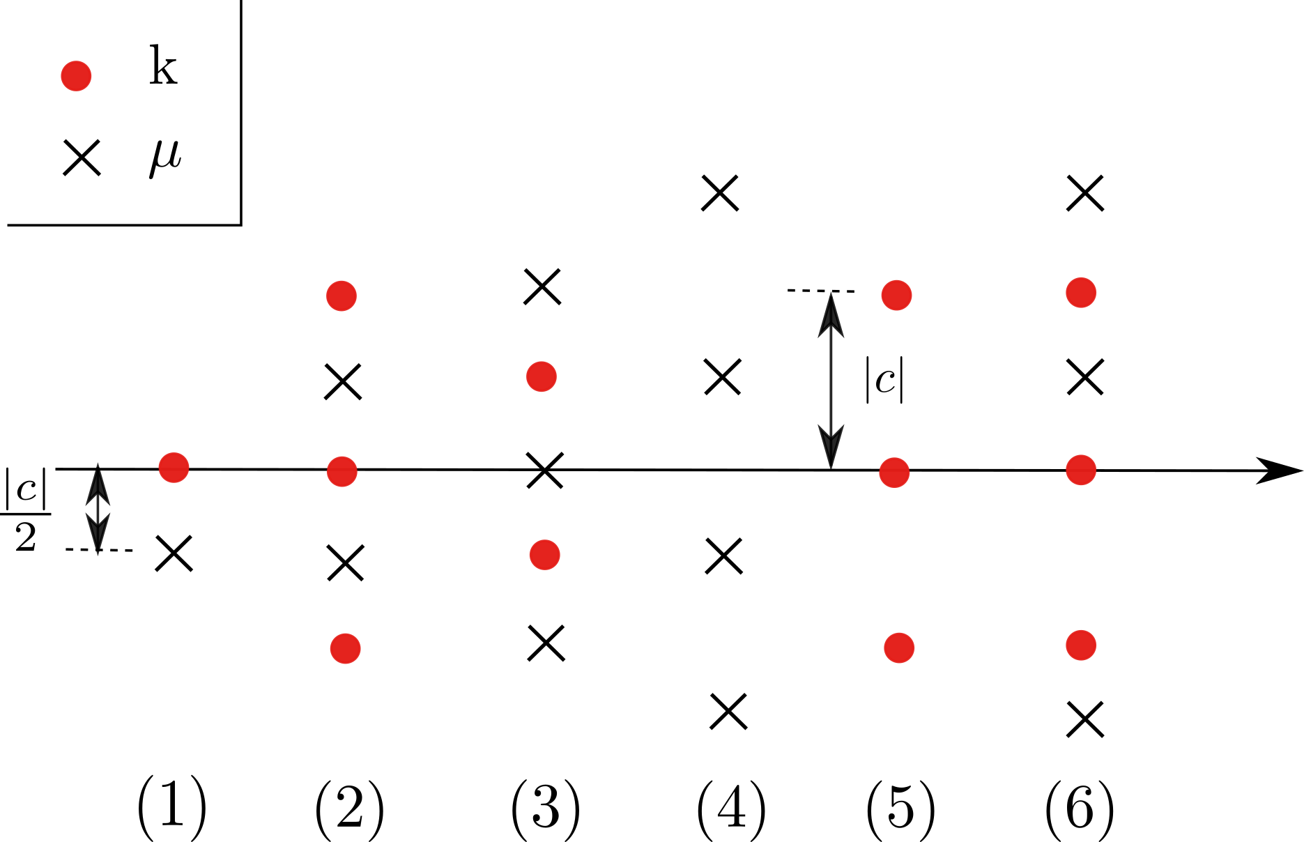
Figure 3 shows an illustration of each type of string solutions. In the String hypothesis, Takahashi predicted the existence of $\mu$ string of any length and $k-\mu$ string of length 2. In this section, we will see strings of the first two as well as the last types emerging by shifting contours. No strings of $\mu$ or $k$ alone exist. $k-\mu$ pair is a basic building block of string solutions, but it does not have any physical significance in real space. $\mu-k$ strings of length $n+1$ is treated as $k-\mu$ string of length $n$ accompanied by two $k-\mu$ pairs. The two strings are physically equivalent. Moreover, we will see that although $\mu-k$ strings of length 2 describes bound state between two down spins, it can be decomposed into sum of free states. For $c<0$, we will also see $k-\mu$ string of length $n>2$, which represents a cluster of $n$ particles bounded together by $n-1$ spin waves.

In order to perform the separation, we first perform the $\mu$ integration. This will result in a constant term plus a sum over terms with Lieb-Liniger type of poles, i.e. $k_{i}-k_{j}+ic=0$ for $i<j$ and $P\raisebox{6.00006pt}{$\scriptscriptstyle-\!1$}i>P\raisebox{6.00006pt}{$\scriptscriptstyle-\!1$}j$. Then one shift all $k$ contours to the real axis. For $c>0$, the pole of $k_{i}=k_{j}-ic$ lies below both $k_{i}$ and $k_{j}$ contours. Thus, no pole is caught when one shift contours to the real axis. For this reason, the only type of string exists, after separating different states apart, is the one with a real $k_{i}$ ($i\leq\beta$ and $P\raisebox{6.00006pt}{$\scriptscriptstyle-\!1$}i\geq\alpha$) and a complex $\mu$ at $k_{i}+ic/2$ (string type 1). However, such string depends on how we close the $\mu$ contours. If we close both contours from below, we are left with a different string configuration with $\mu=k_{j}-ic/2$ for $j\geq\beta$ and $P\raisebox{6.00006pt}{$\scriptscriptstyle-\!1$}j\leq\alpha$. Physically, it should not matter how one closes the contour, as mathematically it leads to the same result. Indeed, they are not related to bound state in real space.

However, we also noticed the appearance or disappearance of a $\mu$-k string of length 2 which depends on how one closes the contour. For the purpose of illustration, we will consider a specific scenario, with $\alpha_{1}=3,\alpha_{2}=2$, $\beta_{1}=2,\beta_{2}=4$, $P=P_{15}$. Under this condition, the integrand of $\mu$ and $k$ becomes

If one closes the contour of $\mu_{1}$ and $\mu_{2}$ from the same direction, there is no $\mu-\mu$ string. But if one closes $\mu_{1}$ from below and $\mu_{2}$ from above, we see four terms corresponding to $\mu_{1}=\mu_{2}+ic=k_{i}+3ic/2$ for $i=1,2,3,4$. What is strange about these solutions is that it leads to a result whose denominator has poles at $k_{i}-k_{j}-2ic$. This is a new type of pole. But the fact is, if we sum up the contribution from these strings, these new poles are canceled by the numerator of the sum. This means, the sum of the $\mu$ strings is equivalent to a collection of states without strings. Physically, that means the bound state between two down spins can be decomposed into sum of free states. As the energy does not depend on $\mu$’s, the bound states keep a coherence phase with all other states. Thus, it is impossible to tell whether the decrease of the wavefunction as the two impurities separate is due to bound states or simply destructive interference among free states. That is to say, the $\mu$ string does not play an important role in real space. As there is no $k$ strings when $c>0$, there is no bound states in such system.

When $c<0$, the pole of $k_{i}$ at $k_{j}-ic$ is between the contours of $k_{i}$ and $k_{j}$. When shifting both contour to the real axis, the original integral splits into two terms. One results from the residue, the other one is integrated along the real axis. The former describes a bound state and the other is a free state, see [5]. As the appearance of this pole originates from the residue at $\mu_{m}=k_{i}+ic/2$, such pole contribution yields bonds among $k_{i}$, $\mu_{m}$ and $k_{j}$. Since no two $k$’s can take the same value, each $\mu$ connects at most two $k$’s. However when different $\mu$’s relate to a same $k$, it will snap two $k-\mu$ strings together to form a longer string. Such $k-\mu$ string solutions of length greater than 2 are not included in the String hypothesis, as it involves ambiguity of $0/0$ in the Bethe equations Eq. (II.6) and (II.7). However, they do exist in the time evolution of the system. Figure 4 shows a complete set of string solutions in the example considered here.

In order to interpret these string solutions, we keep track of the particles by their quasimomentum $k$’s. In the above example, we have $P=P_{15}$, thus particle $k_{1}$ switches position with particle $k_{5}$. In the final state, particle $k_{Pi}$ becomes the $i$th particle in the sequence. $P\raisebox{6.00006pt}{$\scriptscriptstyle-\!1$}i$ is the location of the particle $k_{i}$ in the state.

When $P\alpha=\beta$, i.e. the down spins stays with the original particles, the integral does not vanish under any circumstances. However when $P\alpha<\beta$, i.e. the down spin transfers to a prior particle labeled by $k_{P\alpha}$, the integral will vanish unless there exists a $k_{Pi}$ such that $i<\alpha$ and $Pi\geq\beta$. This indicates that a particle may acquire the down spin in two ways. Either the impurity itself crosses the target particle or the particle after $\beta$ first passes the impurity and then pass the target particle.

Besides transferring down spins, the interaction can also lead to bound states. In order to form a bound state between particle $i$ and $j$, the following condition must be satisfied $i\leq\beta\leq j$ and $P\raisebox{6.00006pt}{$\scriptscriptstyle-\!1$}i\geq\alpha\geq P\raisebox{6.00006pt}{$\scriptscriptstyle-\!1$}j$. Physically, this means one of the following situations depicted in table 1. When a bound state involves an up spin and a down spin, it is a singlet which is related to Cooper pair in BCS and FFLO state. When the bound state includes two up spins, it is a triplet and describes a bound state in a normal state.

As shown in [3], in an unpolarized system, the singlet bound state leads to Cooper pairs in the weak interaction regime, and it relates to the bound state with bosonic nature that results in BEC with strong attraction. When the spin is unbalanced, the string solution characterizes FFLO states. However, the bound state that is described by the string solution, is not a cooper pair in BCS or FFLO state by itself. The center of mass momentum of the former is determined by the spin rapidity, while that of the latter equals zero or the difference between the Fermi wave vectors. In fact, the Cooper pair is a dressed version of the bound state described by the string solution. That is to say, changing one string solution will affect the position of other strings as determined by the Bethe equation. And the cooper pair describes the collective behavior of the whole system. When the spin is unpolarized, breaking a string does not change the total momentum as the other string will shift their center accordingly to minimize the energy and remain symmetric on the momentum axis. The situation is different when there are unpaired fermions, which interact differently with the strings. Thus breaking a string will change the total momentum, making the momentum of the dressed bound state nonzero. Here we only provide an intuitive picture between the string solutions and the Cooper pair. The explicit relation between them is still elusive. But one can tell that the existence of the singlet solution is a necessary condition to the emergence of the FFLO state.

Here we want to remark that the situation is quite different in a quench dynamic where the system no longer seeks the lowest energy state. Instead, each string solution evolves independently with the weight determined by the overlap. Due to the abundance of excitation in the nonequilibrium dynamics, the FFLO quasiparticle picture does not hold. Indeed, as shown in [36], the pair correlation loses the FFLO signature quickly after turning off the longitudinal confinement potential.

Aside from bound states between two particles, more particles can bind together via more spin wave modes. In the example in Figure 4e, $k_{1}$, $k_{2}$ and $k_{5}$ forms a bound state with the help of $\mu_{1}$ and $\mu_{2}$. In order to form such a bound state, one needs to reverse the order of particle 1,2,4 and 5. Though particle 4 does not show up in the bound state, the spacial motion of it relative to the particles in the bound state is crucial to the formation of it. Moreover, as particle 4 is sandwiched between particle 2 and particle 5, the wavefunction will also decrease exponentially with the separation between particle 4 and 2 as well as particle 4 and 5. However, such binds are different to that among $k_{1}$, $k_{2}$ and $k_{5}$. The wavefunction of this bound state consists of the factor $\exp(ik(y_{P\raisebox{2.3917pt}{\tiny-\!1}1}-x_{1}+y_{P\raisebox{2.3917pt}{\tiny-\!1}2}-x_{2}+y_{P\raisebox{2.3917pt}{\tiny-\!1}5}-x_{5})+c/2(y_{P\raisebox{2.3917pt}{\tiny-\!1}1}-x_{1}-y_{P\raisebox{2.3917pt}{\tiny-\!1}5}+x_{5}))$ $\exp(ik_{4}(y_{P\raisebox{2.3917pt}{\tiny-\!1}4}-x_{4}))$. Therefore, although particle 4 is bounded with particle 1,2 and 5, it does not move coherently with them and its quasimomentum is different from that of the center of mass of the bound state. Note, such bound state cannot be decomposed into two bound states related to shorter strings, which should take the form $\exp((ik(y_{P\raisebox{2.3917pt}{\tiny-\!1}1}-x_{1}+2y_{P\raisebox{2.3917pt}{\tiny-\!1}2}-2x_{2}+iy_{P\raisebox{2.3917pt}{\tiny-\!1}5}-x_{5})+c/2(y_{P\raisebox{2.3917pt}{\tiny-\!1}1}-x_{1}-y_{P\raisebox{2.3917pt}{\tiny-\!1}5}-x_{5}))$. Thus, in the String hypothesis, one should include $k-\mu$ strings of all lengths.

References

- [1] Y.-a. Liao, A. S. C. Rittner, T. Paprotta, W. Li, G. B. Partridge, R. G. Hulet, S. K. Baur, and E. J. Mueller, Nature 467, 567 (2010).
- [2] H. Moritz, T. Stöferle, K. Günter, M. Köhl, and T. Esslinger, Physical review letters 94, 210401 (2005).
- [3] X.-W. Guan, M. T. Batchelor, and C. Lee, Reviews of Modern Physics 85, 1633 (2013).
- [4] M. Takahashi, in Exactly Solvable Models Of Strongly Correlated Electrons (World Scientific, 1994), pp. 388–406.
- [5] D. Iyer and N. Andrei, Physical review letters 109, 115304 (2012).
- [6] D. Iyer, H. Guan, and N. Andrei, Physical Review A 87, 053628 (2013).
- [7] W. Liu and N. Andrei, Physical review letters 112, 257204 (2014).
- [8] C. Destri and J. Lowenstein, Nuclear Physics B 205, 369 (1982).
- [9] J.-S. Caux, Journal of Statistical Mechanics: Theory and Experiment 2016, 064006 (2016).
- [10] J.-S. Caux, Journal of Mathematical Physics 50, 095214 (2009).
- [11] A. E. Feiguin and S. R. White, Physical Review B 72, 220401 (2005).
- [12] F. Essler, S. Kehrein, S. Manmana, and N. Robinson, Physical Review B 89, 165104 (2014).
- [13] F. Schwarz, I. Weymann, J. von Delft, and A. Weichselbaum, arXiv preprint arXiv:1708.06315 (2017).
- [14] P. R. Zangara, A. D. Dente, E. Torres-Herrera, H. M. Pastawski, A. Iucci, and L. F. Santos, Physical Review E 88, 032913 (2013).
- [15] J. Zhang, C. Shen, and W. Liu, Physical Review A 83, 063622 (2011).
- [16] O. Kashuba, D. M. Kennes, M. Pletyukhov, V. Meden, and H. Schoeller, Physical Review B 88, 165133 (2013).
- [17] M. Heyl and S. Kehrein, Journal of Physics: Condensed Matter 22, 345604 (2010).
- [18] open-source time-evolving block decimation, URL http://physics.mines.edu/downloads/software/tebd.
- [19] A. Feiguin, F. Heidrich-Meisner, G. Orso, and W. Zwerger, in The BCS-BEC Crossover and the Unitary Fermi Gas (Springer, 2012), pp. 503–532.
- [20] C. N. Yang, Phys. Rev. Lett. 19, 1312 (1967), URL https://link.aps.org/doi/10.1103/PhysRevLett.19.1312.
- [21] M. Gaudin, Physics Letters A 24, 55 (1967).
- [22] M. Takahashi, Progress of Theoretical Physics 47, 69 (1972).
- [23] M. Fowler and X. Zotos, Physical Review B 24, 2634 (1981).
- [24] N. Andrei, K. Furuya, and J. Lowenstein, Reviews of modern physics 55, 331 (1983).
- [25] A. Tsvelick and P. Wiegmann, Advances in Physics 32, 453 (1983).
- [26] J. Lee and X.-W. Guan, Nuclear Physics B 853, 125 (2011).
- [27] H. Hu, X.-J. Liu, and P. D. Drummond, Physical review letters 98, 070403 (2007).
- [28] V. Yudson, ZHURNAL EKSPERIMENTALNOI I TEORETICHESKOI FIZIKI 88, 1757 (1985).
- [29] V. Yudson, Physics Letters A 129, 17 (1988).
- [30] G. Goldstein and N. Andrei, arXiv preprint arXiv:1309.3471 (2013).
- [31] G. Goldstein and N. Andrei, Physical Review B 92, 155103 (2015).
- [32] C. Rylands and N. Andrei, arXiv preprint arXiv:1408.3652 (2014).
- [33] D. Braak and N. Andrei, Journal of Statistical Physics 105, 677 (2001).
- [34] F. H. Essler, H. Frahm, F. Göhmann, A. Klümper, and V. E. Korepin, The one-dimensional Hubbard model (Cambridge University Press, 2005).
- [35] V. E. Korepin, N. M. Bogoliubov, and A. G. Izergin, Quantum inverse scattering method and correlation functions, vol. 3 (Cambridge university press, 1997).
- [36] C. Bolech, F. Heidrich-Meisner, S. Langer, I. McCulloch, G. Orso, and M. Rigol, Physical review letters 109, 110602 (2012).
- [37] N. J. Robinson, J.-S. Caux, and R. M. Konik, arXiv preprint arXiv:1602.05532 (2016a).
- [38] N. J. Robinson, J.-S. Caux, and R. M. Konik, Physical review letters 116, 145302 (2016b).
- [39] DLMF, NIST Digital Library of Mathematical Functions, http://dlmf.nist.gov/, Release 1.0.16 of 2017-09-18 (2017), f. W. J. Olver, A. B. Olde Daalhuis, D. W. Lozier, B. I. Schneider, R. F. Boisvert, C. W. Clark, B. R. Miller and B. V. Saunders, eds., URL http://dlmf.nist.gov/.
- [40] T. Rom, T. Best, D. Van Oosten, U. Schneider, S. Fölling, B. Paredes, and I. Bloch, arXiv preprint cond-mat/0611561 (2006).