A Physical Model for the Spectral-Timing Properties of Accreting Black Holes
Abstract
We develop new techniques to deconvolve the radial structure of the X-ray emission region in the bright low/hard state of the black hole Cygnus X-1 using both spectral and timing data in the 3-35 keV range. The spectrum at these energies is dominated by Comptonisation rather than the disc, but there is a complex pattern in the time lags between different energy bands and differences in the normalisation and shape in the power spectra of these bands, which clearly shows that the Comptonisation is not produced from a single, homogeneous region. We use a physically based model of density fluctuations propagating through a spectrally inhomogeneous flow, setting the spectral components by jointly fitting to the time-averaged and Fourier resolved spectra. The predicted variability in any band is modelled analytically in Fourier space so it can be fit directly to the observed power spectra and lags. We find that the best fit model picks out three distinct radii in the flow, each with a distinct Compton spectrum. The variability and luminosity produced at these radii is enhanced, while propagation of fluctuations from larger radii is suppressed. We associate these radii with the disc truncation, the inner edge of the flow, and (more speculatively) the jet launch radius. These distinct radii are most evident where the source is close to a transition between the low/hard and high/soft states. We suggest that the smoother power spectra seen at lower luminosities imply that the source structure is simpler away from the transition.
Keywords:
accretion, accretion discs – X-rays: binaries – X-rays: individual: Cygnus X-11 Introduction
The overall spectral properties of the low/hard state in black hole binaries (BHBs) are often interpreted in a truncated disc/hot inner flow geometry (see e.g. the review by Done, Gierliński & Kubota 2007; hereafter DGK07). In this picture, a cool, optically thick, geometrically thin disc (Shakura & Sunyaev 1973) transitions at some radius to a hot, optically thin, geometrically thick inner flow which behaves similarly to an advection-dominated accretion flow (ADAF; Narayan & Yi 1995). A decreasing truncation radius between the cool disc and the hot, inner flow as the mass accretion rate increases (on timescales of days to weeks) leads to stronger disc emission, and hence stronger Compton cooling of the hot flow, so that its spectrum steepens. This also provides a mechanism to explain the transition to the disc-dominated state when the truncated disc finally reaches the innermost stable circular orbit (ISCO; Esin, McClintock & Narayan 1997; DGK07).
More recent work has shown in detail how this can also explain the properties of the fast variability (on timescales of s), including the strong low frequency quasi-periodic oscillation (QPO). The radius of the thin truncated disc sets the outer radius of the hot inner flow. Any turbulence in the hot flow will have a timescale which decreases with radius, so the longest timescale fast variability is set by the outer radius of the hot flow (Lyubarskii 1997; Arévalo & Uttley 2006); this defines the low-frequency break in the power spectrum. The QPO can be produced in the same geometry by Lense-Thirring (relativisitic vertical) precession of the entire hot flow (Fragile et al. 2007; Ingram et al. 2009), predicting that the iron line centroid energy is modulated on the same quasi-period as the QPO. This characteristic signature of prograde precession has been seen in the data in H1743-322 ( detection; Ingram et al. 2016). The decrease in truncation radius with increasing mass accretion rate which produces the spectral softening then also drives the correlated decrease in low frequency break and QPO timescale, as observed (Wijnands & van der Klis 1999; Klein-Wolt & van der Klis 2008; Ingram & Done 2012b).
This geometry also offers a qualitative explanation of the more complex, higher order variability properties. It is well established that BHB lightcurves on fast timescales show variability in higher energy bands lagging behind that from lower energy bands (Miyamoto & Kitamoto 1989; Nowak et al. 1999; Grinberg et al. 2014). These lags might be expected in a model where the low energy band is dominated by the disc, and the high energy band is dominated by Comptonisation from the hot flow. Fluctuations in the disc will propagate inwards through the hot flow, but with some lag time corresponding to the viscous timescale for the fluctuation to drift from the disc inner edge to the innermost parts of the hot flow which dominate the Comptonised emissivity (Uttley et al. 2014;Rapisarda et al. 2016). However, such models are unable to explain why these lags are seen between different energy bands where the disc emission is negligible, nor why the lags also depend on the frequency of variability (Nowak et al. 1999; De Marco et al. 2015; Misra et al. 2017). Instead these features can be explained if the hot flow itself is stratified not only in variability timescale, but also in spectral shape, such that the outer regions of the flow are associated with softer Compton spectra than the inner regions (Kotov, Churazov & Gilfanov 2001; Gierliński, Done & Page 2009). Slow variability is generated at the largest radii, in the region where the Compton spectrum is softer. These fluctuations have the largest distance to travel (i.e. the longest lag time) before they modulate the hardest spectral inner regions. By comparison, faster variability is produced closer in, so has a shorter distance to propagate - and hence a shorter lag time - before it modulates the spectrally hardest inner regions (Mahmoud & Done 2018, hereafter MD18a). If instead the hot flow were homogeneous, spectra from the outer and inner radii would be the same, so while the fluctuation in the inner radii would be lagged behind those produced in the outer radii, two different energy bands would each sample the same fraction of initial and lagged emission, so their lightcurves would be the same, and no lag would be observed.
Thus the observed lag between different energy bands which are both dominated by Comptonisation suggests that the spectral and variability properties of the hot flow are radially stratified. The observed spectral variability can therefore in principle be used to determine the radial stratification of the hot flow. This goal is complementary to that of the recent work of Mastroserio, Ingram & van der Klis (2018), where they focus on using the continuum variability to probe the thin disc structure via reverberation. Here we are interested instead in using the continuum variability to probe the continuum source itself.
We develop techniques to use the observed spectral-timing information to build a model of a flow which is radially stratified in variability, emissivity and energy spectra, developing significantly from our previous work in MD18a. We use this on some of the best available data, that of the Rossi X-ray Timing Explorer (RXTE) observations of Cyg X-1, taken before the telemetry limitations which accompanied the antenna failure. Cygnus X-1 is an ideal source for this study, since there is no obvious QPO to complicate the underlying propagation models, as well as being very bright, resulting in a high signal-to-noise. We show simultaneous fits to the time averaged spectra, the frequency resolved spectra, and the power spectral densities (PSDs) over different energy bands, together with the lags between those energy bands. We show that we can build a self-consistent picture of all these data with a flow composed of two spectral regions, with the transition from soft to hard spectra at very small radii (within of the black hole) associated with a large peak in both the variability and the emissivity. Alternatively, we prefer a three component spectral model which gives larger radii, with maximal variability and emissivity generated in an intermediary region from . While we cannot break all the degeneracies, we show that the data fundamentally require spectrally distinct regions within the Comptonisation zone, and that the variability and emissivity are jointly enhanced at specific radii. In this picture, the flow consists of a number of bright, turbulent rings rather than being a smooth, self-similar structure. This picture is very different to the original assumption that variability is dominated by the radially smooth turbulence of the Magneto-Rotational Instability (MRI), which remains the physical mechanism behind the angular momentum transport in the flow (e.g. Balbus & Hawley 1998, Noble & Krolik 2009, as used by Ingram & Done 2011, hereafter ID11; Ingram & Done 2012a). The bright, turbulent radii we identify must be important in understanding the physics of the flow, and we suggest identifying these with the disc truncation radius, the ‘bending wave’ or nonaxisymmetric tilt-shock radii seen in Magnetohydrodynamic simulations (MHD; Lubow, Ogilvie & Pringle 2002; Fragile et al. 2007; Generozov et al. 2014), and/or the jet launch radius.
We note that this complex source structure is required by the distinct timescales picked out by the multiple separate maxima (‘humps’) in the power spectra. A systematic analysis of all the RXTE PCA data shows that these separate components in the power spectra are especially evident in the intermediate states, where the source is making a transition between the low/hard and high/soft states (Belloni et al. 2002; Axelsson et al. 2005, Grinberg et al. 2014). Instead, the power spectra are much smoother in the dimmer low/hard states, indicating that the X-ray emitting Comptonisation source structure may be described by simpler models where there is a smooth radial gradient in variability timescale, amplitude, emission spectrum and luminosity in these states (Rapisarda, Ingram & van der Klis 2017a, hereafter R17a). We will apply these spectral-timing techniques to data from a dim low/hard state data in a subsequent paper (Mahmoud, Done & De Marco, in preparation).
2 Analytic Modelling
In the following we denote radii as , with gravitational radius and black hole mass .
In MD18a we carried out all simulations of the mass accretion variability in the hot flow using a numerical procedure adapted from the method of AU06 and ID11. In that method, the mass accretion rate curve in each annulus, , was generated by randomly sampling from a zero-centered Lorentzian with a cut off at the local viscous frequency, ,
| (1) |
here is the fractional variability per radial decade at , related to the rms variability produced at via , where is the number of annuli per radial decade. The samples were then transformed to the time domain via the Timmer and König (1995; hereafter TK95) algorithm. These mass accretion rate curves were then lagged and multipled together to simulate propagation through the flow, and the final time series were weight-summed to produce the light curves in each band.
However these simulations are slow. The basis for a fast procedure to produce the energy-dependent PSDs was also adapted in MD18a from the groundbreaking analytic formalism of Ingram & van der Klis 2013, hereafter IvdK13. This analytical method can produce results consistent with those of the TK95 algorithm when spectral constraints are also included. In this work we will use this faster technique to enable us to search through the wide parameter space generated by the multiple components of the model. The updated formalism is described in rigorous detail in Appendix A, but we give an overview of the physical parameters below.
2.1 Spectral Stratification
Fundamentally, our model assumes a changing spectral shape as a function of radius, . In the simplest case, it describes a hot flow stratified into two regions, each of which produces a different spectral shape. A soft spectral component, , is produced in the outer region, while the inner region produces a hard spectral component . In this work, both of these components are formed from Comptonisation as the RXTE PCA is sensitive only above 3 keV, where the disc emission is neglible. This is different to the two component models used by Rapisarda, Ingram & van der Klis (2017a), where the lower bandpass of XMM-Newton means that they are sensitive to the direct emission from the disc. Their two component model describes a disc and homogeneous hot flow, while ours describes an inhomogeneous hot flow.
, and their reflected components are determined from direct fitting of a two Compton component model to the broadband spectrum, further details of which are described in Section 4. For soft and hard Comptonisation components (and their reflections) , , and , the time-averaged spectrum associated with each annulus is given by
| (2) |
here is the transition radius between the soft and hard Comptonisation regions. This is analytically derived from the radial scale, the spectral components and , and the prescribed emissivity (parameterised in Section 2.3) such that the luminosity ratio between the two direct components, , matches that of the emissivity, via
| (3) |
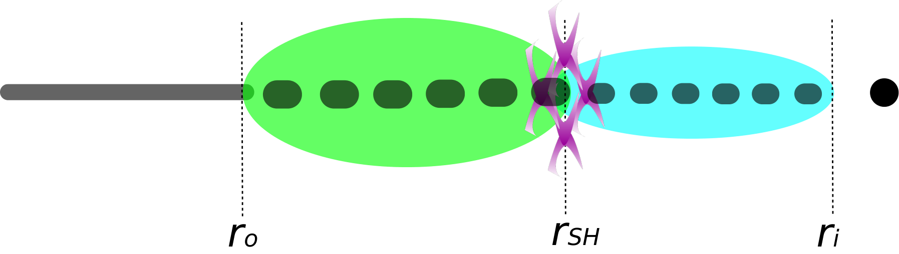
Regarding equation (2), we note that our model assumes that the observed variability relates only to variation in the normalisation of each spectral component, not from a changing spectral shape. This means we assume that the seed photon rate for Comptonisation changes with in the flow, because the spectral index is set by the balance between electron heating from and cooling from the seed photons (e.g. Beloborodov 1999). Any change in the heating and cooling can lead to changes in spectral index of the Comptonisation spectrum. The heating and cooling are expected to vary together if the seed photons are predominantly from disc-reprocessed X-ray emission (Haardt & Maraschi 1993) and the light travel time for this reprocessing is fast compared to the propagation time. The latter is fairly well justified for our parameters since the disc truncation radii we derive here from the QPO-low frequency break relation (ID11; Section 2.2) are all <, equating to a light travel time of order ms. Of course this is not always the case for AGN (Gardner & Done 2014).
However, if the seed photons for the Hard component instead originate from the Soft Compton component, then there will be correlated but lagged variability between the dissipation in the inner regions and its seed photons caused by the same fluctuation which appeared earlier in the outer regions. Alternatively (or additionally), changes in spectral shape can be produced even if the seed photons are locally generated, if they arise via cyclo-synchrotron emission. An increase in density gives rise to more local dissipation but fewer seed photons as it increases the synchrotron self absorption. This would result in a simultaneous (no lag) anticorrelation of the seed photons with . Both cases would lead to strong spectral pivoting (Veledina 2016).
Nonetheless, spectral pivoting alone (with or without lags) is not likely to explain all of the lags seen in the Cyg X-1 dataset. Mushtukov, Ingram & van der Klis (2017) used spectral pivoting to fit to the complex covariance of this Cyg X-1 data. Here their focus was to phenomenologically model the continuum lags in order to extract the reverberation lags from the disc. They derived an extremely small inferred inner radius for the disc of , but with significant residuals around the iron line. This suggests that their model is using the reverberation lags to compensate for continuum lags which are not modelled with their purely pivoting continuum approach. We caution that a full picture of the spectral-timing properties of the flow may require a combination of all these factors, and we will explore this in future work.
Once , , and are established from the spectrum, the model then solves for parameters which set the radial dependencies of the flow, including
- 1.
The radial propagation speed
- 2.
The fractional variability per radial decade,
- 3.
The total emissivity,
- 4.
Propagation losses of variability amplitude. This occurs due to either smoothing by the Green’s function response of the flow, and/or damping due to macroscopic turbulent processes.
We specify these parameters in detail below, using previous results as the basis to set the minimum number of free parameters required to reproduce the features seen in these data.
2.2 Propagation Speed
In simple propagating fluctuations models, the viscous frequency often follows where is the Keplerian frequency. This sets the frequency at which fluctuations are generated at through equation (1). Here we assume that this also sets the propagation speed, , through . As we show in Appendix C, the viscous timescale therefore determines not only the peak positions in the PSD, but also the time lag between energy bands.
In MD18a, we used the association of the low frequency QPO with Lense-Thirring precession (see Ingram et al. 2016) to set and . This was required to reproduce the relation between the low frequency power spectral break and the QPO frequency (-; ID11). This relation correlates the low-frequency noise near - that generated in the outermost regions of the flow - with the QPO frequency assuming solid-body precession of the entire hot flow.
However the low frequency break could instead be set by fluctuations from the inner edge of the disc rather than fluctuations in the hot flow itself. In this work, we therefore assume that and in the outer part of the flow, but we also explore whether the inner flow has a distinct propagation speed, as might be expected from the transition between the thin disc and the hot flow (Hogg & Reynolds 2017). Where the spectral shape switches from soft to hard, the physical process resulting in the different spectrum may also be associated with a different viscosity form. We therefore parameterise the viscous timescale as
| (4) |
where , , and are model parameters for the viscosity in the soft and hard regions. Regardless of the internal variability processes of the flow at , the - relation should hold, so we fix and . However we do allow and to vary, as the inner-region viscosity is not constrained by the QPO.
We note that some previous works (e.g. Ingram & Done 2012a, Rapisarda et al. 2016, R17a) have instead used a viscous frequency profile for the flow which smoothly varies with surface density, this form being inferred from MHD simulations. However those works also assume smooth, MRI-driven turbulence and emission profiles, as these were satisfactory to explain their data given the lack of spectral constraints. In the new picture we are exploring - of quasi-limited regions enhancing the variability, and in particular of the thin disc being shredded in the soft region - it becomes inconsistent to think of the viscous timescale as being a smooth function of radius. This motivates the broken profile of equation (4).
2.3 Correlated Turbulence and Emissivity in a 2-Component Flow
MD18a principally showed that the ‘bumpy’ power spectra seen in the brighter low/hard states of Cyg X-1 and other sources (Churazov, Gilfanov & Revnivtsev 2001; Pottschmidt et al. 2003; Axelsson et al. 2008; Torii et al. 2011; Misra et al. 2017; GX 339-4: Nowak 2000) cannot be matched by self-similar turbulence where is constant. Regions of enhanced variability over a very small range in radii are required in order to produce an excess of power over a limited frequency range. These may be physically associated with the transition from the thin disc to the hot flow, nonaxisymmetric shocks at the inner radius of the flow if this is tilted with respect to the black hole spin (Henisey, Blaes & Fragile 2012; Generozov et al. 2014) or the jet/flow interaction.
The PSDs in our data show three distinct bumps (the shaded regions in e.g. Fig. 4a). In an effort to reproduce the clearly complex structure seen in the variability, we would like a phenomenological model for the turbulence as a function of radius which does not require an excess of free parameters. We therefore parameterise as a sum of three gaussians, with width, , radial position, and amplitude, , giving
| (5) |
One very natural source of this variability is at the truncation radius, where the interaction between the between the Keplerian disc and sub-Keplerian flow is likely to be highly unstable. We therefore associate the outermost gaussian in with the truncation radius so that . We also impose joint constraints on the other parameters in equation (5). The characteristic radii of the two inner gaussians are always limited to be less than that of the adjacent outer one, i.e. and < . also cannot fall below the inner radius of the flow, so that . We force positive-definite resulting lightcurves by ensuring that the rms variability generated in any region has . Models which go above this limit are flagged as infinitely bad in terms of goodness of fit (see Section 3). Since , this implies joint upper boundaries on the gaussian widths and amplitudes, and .
Incorporating equation (5) into the model allows it the freedom to significantly vary the amount of turbulence within the flow as a function of position. The physical pictures which can be inferred from the fits can therefore range from the traditional propagating fluctuations model, with broad, low amplitude Lorentzians producing constant variability at each radial decade, to the case of certain processes dominating the variability at distinct radii, potentially independent of any smooth MRI-driven turbulence.
However, to make an impact on the power spectra, regions of enhanced variability should form a significant contribution to the resulting lightcurves. This requires that they modulate a large fraction of the total luminosity. It is difficult to do this with a smooth emissivity (as assumed in MD18a) as this limits the contribution to the lightcurve from any small range of radii. The impact of a turbulent region in the lightcurve is a product of the variabilty power and the integrated emissivity over the radial range where the enhanced variability appears. With the smooth emissivity assumption, the additional variability required to fit the data is so large that the assumption of linearity in the generated lightcurves is broken (MD18a). This results in the lightcurves becoming negative, which is unphysical!
We now link the turbulence to the emissivity of the flow, such that the more variable regions produce a larger proportion of the emission. This is motivated not only by the demands of the data, but also by the findings of MHD simulations which show that turbulence is inherently dissipative (see e.g. Blaes 2013). We parameterise the radial dependence of the emissivity with a sum of three Gaussians, tied to the same radii and width as for the turbulence above, but with free normalisations. We also assume that this occurs on thebackground of a smooth with index in order to encode the joint contributions from the turbulence and gravitational energy release to the energetic dissipation. We then have
| (6) |
where and are the relative amplitudes of the second and third Gaussians to that of of the outermost at . Through equation 6, the model can also encompass interference-based interpretations of the double-humped power spectra, where the correlated, lagged variability between Comptonised photons from the outer and inner regions results in suppressed power in the range of frequencies for which the lag is half of the fluctuation period (Veledina 2016). On the other hand if interference is not significant, i.e. if the propagation delay is too short, damping will be required to suppress the propagated power and produce dips in the power spectra (see Section 2.4).
To calculate light curves in different energy bands from our simulation, we weight the mass accretion rate at each annulus by the product of the emissivity at , and the integrated spectral components of equation (2), folded with the detector response and interstellar absorption (see equation 21). Including the detector response and interstellar absorption ensures that the simulated data is weighted in the same way as the observations.
In Fig. 2(a) & (b) we show the schematic for the revised and profiles with arbitrary normalisation on both, illustrating how these profiles are now associated in terms of the positions and radial scales of the enhanced regions.
2.4 Smoothing and Damping
Another key feature often seen in the Cyg X-1 low/hard states which previous models have been unable to replicate is the suppression of low-frequency correlated variability associated with lower energy bands compared to higher energy bands (e.g. Grinberg et al. 2014, Rapisarda, Ingram & van der Klis 2017b; MD18a). This feature is also seen in other BHBs including SWIFT J1753.5-0127 and GX 339-4 (Wilkinson & Uttley 2009), and so is likely generic to the low/hard state paradigm. For similar Low and High energy power spectral shapes (i.e. no preferential suppression of certain frequencies between bands), the timing properties can be jointly fit using simple propagating fluctuations, but when the power spectral shapes become distinct at low frequencies, the lags in each band become dominated by different spectral components and joint fits fail (Rapisarda, Ingram & van der Klis 2017a). This implies that the variability present in the spectrally softer regions is not completely propagated down to modulate the harder regions. Yet the fact that there are lags between Low and High bands on the timescale of the outer parts of the flow means that at least some of the variability does propagate. The variations in the soft region must therefore map onto the inner-region variability after propagation, although with smaller amplitude and a time delay.
Our model includes two distinct methods of variability suppression. First, there can be diffusion of fluctuations as they propagate through the flow due to the Green’s function response (e.g. R17a). This acts to preferentially smooth out the fluctuations which have propagated over a larger distance compared to their wavelength. We follow R17a and model this as an exponetial decay such that all fluctuations of frequency which propagate from to (which takes timescale ) are suppressed by a continuous factor . Here
| (7) |
However, our model fundamentally includes regions of enhanced variability/emissivity. The specific processes which generate this additional power could also suppress the propagating fluctuations at the associated radii. In our nomenclature, we will refer to the process of suppressing power at all frequencies uniformly at specific radii as ‘damping’, distinct from the diffusive ‘smoothing’ process discussed above, which instead has a frequency/travel time dependence. We tie our damping effect to the radius at which the spectral shape changes from soft to hard. There are two proposed mechanisms by which such damping could occur, the first being an increased density of magnetic field lines at the transition radius. This buildup of flux density could be associated with the jet collimation, or warps induced by the flow tilt with respect to the disc plane. Such a process would be highly disruptive to incoming mass accretion rate fluctuations from . The purple knots in the flow in Fig. 1 represent this concentration of flux density at the spectral transition radius. An alternative, possibly concurrent mechanism which would result in fluctuation damping could be the dissipation of thermal clumps propagating through the flow. Physically, the spectral transition requires a change in seed photon availablity, and these seed photons in the soft region could be from clumps torn from the inner edge of the truncated disc by the truncation process. These clumps would produce copious, highly variable, seed photons for the soft region of the flow, making the characteristic soft, highly variable spectrum (see also Uttley et al. 2011; Grinberg et al. 2014). However as it accretes, a given clump would likely shrink due to its outer layers thermalising with the surrounding medium, and being stripped away by the MRI; this would also result in seed photon starvation of the inner region, explaining the observed hardening of the spectral shape. The grey ‘blobs’ in the flow in Fig. 1 represent these clumps dissipating as they accrete. When considering this possibility however, we bear in mind the work of Poutanen, Veledina & Zdziarski (2018) which showed that synchrotron emission may be the preferred method source of seed photons in the inner flow, although incorporating this into the model would invoke the aforementioned complexity of spectral pivoting.
Applying a generic mechanism which can encompass both magnetically-driven and clump evaporation-driven damping, we suppress all the propagated variabilty by a single factor at the spectral transition radius, . In the context of fluctuations propagating from to , these fluctuations are therefore damped by
| (8) |
In Fig. 2(c) we show an example of these smoothing and damping effects separately, and in combination. Note that the smoothing in this figure is an example for a fixed frequency, , and in truth smoothing acts as a function of frequency.
3 Timing Fit Procedure
Producing a fully generalised model which fits the spectra and timing properties simultaneously would be both technically complex and computationally prohibitive. Furthermore, in a parameter space with dimensions corresponding to the free parameters for both the spectral and timing fits, degeneracy and correlation between parameters would be a significant concern. With this in mind, we fit first to the energy spectra, and then to the energy-dependent timing properties, to demonstrate the possible achievements and limitations of the model. Unlike the slower TK95 method used in MD18a, the fast analytic prescription we use allows us to obtain parameter space minima using the Markov Chain Monte Carlo (MCMC) method via the python package, emcee (Foreman-Mackey et al. 2013). This allows a much more thorough exploration of the parameter space than in MD18a, systematically testing the limits of each model. In all analytic model fits, we assume that Cyg X-1 has a black hole of mass , and a dimensionless spin parameter of 0.85 when calculating (Tomsick et al. 2014; Kawano et al. 2017). All spectral-timing fits use logarithmically spaced radial bins, which is a compromise between computational cost and spatial resolution. We simulate on a time binning of s to match the Nyquist frequency of our data.
To find the timing properties of the data, we extract lightcurves using saextrct in three energy bands: Low (3.13-4.98 keV), Intermediate (9.94-20.09 keV) and High (20.09-34.61 keV). Selecting the boundaries of the Low and Intermediate bands ensures that contamination of the timing signal from the iron line at keV is avoided. Since the PCA response declines rapidly below keV and HEXTE becomes unreliable above keV, these bands span as large an energy range as possible for these data without, significantly sacrificing signal-to-noise. These lightcurves are found by co-addition of three consecutive observations of Cyg X-1 (ObsIDs: 10238-01-08-00, 10238-01-07-000, 10238-01-07-00, hereafter Obs. 1-3), where the similar spectra and hardness ratios of these observations justify their co-addition (see MD18a). Obs. 1-3 all consist of 64 energy bins across the entire RXTE PCA energy bandpass (standard channels 0-249; B_16ms_64M_0_249 configuration) giving moderate spectral resolution in the 3-10 keV band near the iron K line. We calculate the noise-subtracted power spectra and time lags of the data by ensemble averaging over 174 intervals, each containing time bins of s length. The power spectra and time lags are then rebinned geometrically such that the number of points in bin adheres to (van der Klis 1989), with at least a single point in each frequency bin. This produces fully binned power spectra in each band, , and lags between bands, , where and is the number of distinct energy bands. These statistics have corresponding errors , . Since each measured frequency is first ensemble averaged over 174 separate intervals, this far exceeds the prerequisite number of points required for the errors to converge to Gaussian at all frequencies (Papadakis & Lawrence 1993), and so chi-squared fitting is appropriate for this data.
When fitting, we wish to maximise our signal-to-noise ratio in the time lag. Due to the closer proximity of the High and Intermediate (and Intermediate and Low) bands, the propagation lag between these bands is inherently smaller, while their errors are the same as that of the High-Low. Particularly in the case of the Intermediate-High band cross-spectrum, the average lag reduces to s, of the order which would be expected for reverberation lags given the geometry of the system. Since the model does not include the reverberation lag here, fitting to these lag spectra would therefore skew the fit statistic towards an underpredicted lag, breaking the fit.
To simultaneously fit to the power spectra and time lags, we therefore reduce the sum of the chi-squared values for the power spectra in the Low, Intermediate and High bands, and a weighted form of the High-Low band time lags, since the High-Low lag gives us the best signal to noise ratio, thus being the most reliable diagnostic of the propagation lag. In particular we weight the lag by a factor of three against the power spectra. Selection of a factor three ensures an equal balance in fit preference between the overall power spectral and lag statistics. The statistic we reduce is therefore
where the superscripts and refer to the model and observational statistics respectively, and subscripts , and refer to the Low, Intermediate and High energy bands respectively.
4 Spectral Fits: Two Compton Components

| Spectrum | † | † | log() | |||||||
| (keV) | (keV) | |||||||||
| Total | ||||||||||
| These are tied. | ||||||||||
In MD18a we fitted the time averaged SED from Obs. 1 alone in xspec (version 12.9.1; Arnaud, Borkowski & Harrington 1996). The model consisted of two Comptonisation components described by tbabs * (nthcomp + nthcomp) (Zdziarski, Johnson & Magdziarz 1996), and their combined reflection, tbabs * (kdblur * xilconv * twocomp), where twocomp is a local model which adds the Comptonisation components together. This fit was motivated by model simplicity, and by similar successful fits to Cyg X-1 spectra (Gierliński et al. 1997; Di Salvo et al. 2001; Makishima et al. 2008; Basak et al. 2017). In MD18a this fit assumed 0.5% errors on the model alone, and no systematic errors on the data.
For the first spectral fit of this paper, we make two key revisions to this approach. First we use a slightly updated version of the MD18a model, instead fitting tbnew_gas * (nthcomp + nthcomp + kdblur * xilconv * (nthcomp + nthcomp))11
1
tnew_gas is the new, faster version of tbabs (Wilms, Allen & McCray 2000), and can be found here:
pulsar.sternwarte.uni-erlangen.de/wilms/research/tbabs., where the reflected components is now separated into its soft and hard components to be consistent with the revised formalism of equation (2). Second, we now add 1% systematic errors to the data only in the PCA range, and assume zero systematic error on the model, as opposed to the zero data-systematic, 0.5% model systematic used in MD18a. This decision is made for consistency with later fits in this paper, which incorporate Fourier-resolved spectra, using 1% PCA systematics as in Axelsson & Done (2018). Like MD18a however, we have followed Makishima et al. (2008) who fix the seed photon temperature for both Compton components to that of the disc at keV, and tie the electron temperatures of both components. We also fix the galactic column density to cm-2 in this and all other fits. Unlike the timing model, we fit the spectrum to Obs. 1 only, as co-addition of spectral data can result in artefacts.
In Fig. 3 we show the broadband spectral fit. The dominant soft (green) and hard (cyan) Compton components are produced from the outer and inner regions of the flow respectively. Also included is the reflection from the soft component (magenta solid), and from the hard component (magenta dashed), but we do not include the intrinsic or reprocessed disc emission as the energy of this is too low to make a significant contribution to the RXTE data above 3 keV. We denote this as spectral model 2C (two component), with full parameters detailed in Table 1. On comparison to the spectral fit of MD18a which found soft and hard spectral indices of 1.8 and 1.25 respectively, it is clear that the spectral picture we have found here is dramatically different in shape, despite the data being identical and the model having no additional complexity. The discrepancy between them therefore arises entirely from the systematic errors assumed. This exemplifies how susceptible spectral data alone are to degeneracy, when no external constraints are imposed from e.g. the timing properties (see also Basak et al. 2017). Due to the constraints on the seed photon and electron temperatures, the quality of spectral fit 2C is fairly poor () although in Section 4.2 we will look at how releasing these constraints can in fact lead to a better fit to the total and Fourier-resolved spectra.
Fig. 4 shows the optimal joint fit to the PSDs of all three energy bands, and to the High-Low band time lags obtained using spectral model 2C. The parameters of this fit are presented in Table 5, along with parameters for all other spectrally-constrained timing fits shown in the body of this paper. The model fits reasonably well to the power spectral properties, matching the higher normalisation of the Low energy band at low frequencies compared to the Intermediate and High, and the switch to lower normalisation above 8 Hz. However, the model has much less of the double hump structure below Hz than is seen in the data in all energy bands. This is despite the freedom to add regions with enhanced variability, emissivity and damping/smoothing, with the best fit radial profiles shown in Fig. 5. This has significant variability in the outer parts of the flow with a hump in at . This variability then propagates down through the soft region, with most contribution to the Low-energy light curve coming from the inner parts of the soft region due to the centrally peaked emission profile. The significant damping (dashed line in the lower panel) between the soft and hard regions (D_SH = 3.3) has then resulted in the correct power spectral hierarchy, with the hard component modulated by only a small part of the low frequency variability propagated from the soft region.There is no significant smoothing associated with the flow (solid blue line in the lower panel).
However, this best fit solution completely underpredicts the lag. By having a centrally peaked emission profile which does not contribute much beyond , the soft variability becomes characterised almost entirely by that near its inner edge close to . This results in a small ‘characteristic’ propagation time from the soft to hard region, far underpredicting the long lags seen in the data (see equation 32 and Fig. 19).
This tension between the power spectra and lag results are likely due to fundamental problems with spectral model 2C, as the weightings from the spectral fit dictate the contributions each energy band will see from each Comptonisation region. Modification of these spectral weights through an alternative spectral fit can therefore drastically alter the shape of the parameter space explored by the timing model. We will therefore now examine what our timing model can achieve when fitting only to the power spectra and time lags, with no prior fit to the energy spectra.
4.1 No Constraints from the Spectrum
Reworking the model to require no prior spectral fit can be done quite simply, by rewriting equation (21). This equation describes the weighting of the mass accretion rate curve from annulus when calculating the light curve in energy band, . Recasting the energy-dependent part of this equation, we get
| (9) |
where is the detector effective area, is the galactic column absorption and is the Thompson cross-section. The summation limits implied here by ‘region’ are to for and to for . Here, denotes the energy band used, and so can take any value from the set [, or ]. denotes the spectral component originating from annulus , so that for , and for . therefore denotes the luminosity produced by spectral component , as seen in energy band, .
Since we have assumed only two Compton components, here can take one of only six values depending on the energy band and radial zone. Explicitly, we have
| (10) |
for each of the three bands. Usefully, the rms normalisation on the power spectra and cross spectra of equations (26) and (27) mean that in calculating timing statistics, we actually require only the ratio of luminosities from each component in each band, = . We can also remove the necessity for a spectral prior in determining by simply allowing (formerly defined by the spectral fit throigh equation 3) to be free. This leaves us with four additional free parameters in the absence of an independent spectral fit: , , , .
| FSW1 | FSW2 | Fixed by | |
|---|---|---|---|
| spectral fit 2CFR | |||
| PSDs, Lags | Fig. 6 | - | Fig. 9 |
The best fit for our model free of spectral constraints is shown in Fig. 6, with fit values for the new parameters shown in Table 2. We denote this ‘free spectral weight’ fit as FSW1. Now free from the constraints of the spectrum, this fit shows remarkable agreement with the data comapared to previous cases. The PSD hierarchies and structure are better reproduced than before, although the sharpness of the high-energy peaks seems to be slightly underpredicted, potentially indicating that the soft component power should directly feed the hard Component through seed photon variations, as well as mass fluctuations. We discuss this idea further in Section 6. Remarkably though, the lag structure is very well matched for the first time, showing that the lag structure can be reproduced by certain regions of the spectral-timing parameter space, but that constraints imposed by the spectral fit have so far prevented this structure from appearing. On examining the final fit values of , and in Table 2, it seems that the spectral picture required by the timing data is that of a soft Compton component which decays monotonically with energy, providing less than contribution to the flux even in the Low energy band. This seems remarkably close to the behaviour of spectral fit 2C, and those of other fitting studies (e.g. Di Salvo et al. 2001; Basak et al. 2017) which have also indicated a hard component which dominates at all energies above keV, with only a minute soft compton contribution at low energies. The glaring problem with this spectral shape becomes clear however when looking at the required ratio of total fluxes in the soft and hard components, . FSW1 requires , while models which give the required behaviour have soft components with no more than of the luminosity of the hard component, e.g. in the case of 2C where . Not accounting for an unexpected sudden upturn in soft Compton contribution below the PCA bandpass then, the values found for the and are in extreme tension. However, previous spectral fitting studies have also lacked a key tool which we can now use to further constrain the spectrum, extracted from the timing data itself. This tool is the Fourier-resolved (phase-resolved) spectrum.
4.2 Constrained by the Fourier Resolved Spectra

| Spectrum | log() | |||||||||||
|---|---|---|---|---|---|---|---|---|---|---|---|---|
| (keV) | (keV) | (keV) | () | |||||||||
| Total | - | |||||||||||
| Slow FR | " | " | " | " | " | " | " | - | " | |||
| Int. FR | " | " | " | " | " | " | " | - | " | |||
| Fast FR | n/a | n/a | n/a | " | " | " | n/a | n/a | n/a | n/a |
To place further constraints on the spectral fit, we now draw on the Fourier-resolved (FR) spectra found using the technique of Axelsson & Done (2018). These spectra are derived from the first, second and third humps in the energy-independent power spectrum of Obs. 1 (designated here as the ‘slow’, ‘intermediate’ and ‘fast’ variability respectively). In Fig. 7, the slow, intermediate and fast FR spectra are shown as the red, green and blue crosses respectively.
The most obvious fact on comparison of the FR spectra is that the fast component is highly distinct from the other two, with a much steeper slope down to its minimum resolved energy. Since this fast variability corresponds to where is highest, it must derive from the innermost, and therefore the hardest, region. The fast FR component therefore provides a strong constraint on the shape of the hard Compton component, showing that its seed photon temperature, , should be much higher than that of the soft, which draws from the (shredding) disc at keV. If the seed photons for the hard component are coming from a source other than the disc (e.g. the soft region), then the hard region cannot have a line of sight to the disc. If the hard region cannot intercept the photons from the disc, then the disc in turn must not intercept photons from the hard region, and so there is no way that the hard component can produce disc reflection. In the following spectral fits, we therefore switch off reflection from the hard component [=0], in order to keep the spectral model self-consistent.
We now simultaneously fit to the broadband energy spectrum of Obs. 1 and its FR spectra, using 1% systematic errors in the PCA bandpass to ensure consistency with Axelsson & Done (2018). Unlike spectral fit 2C, we allow the hard component seed photon temperature to be free, and untie the soft and hard electron temperatures. Since the slow variablity is produced in the outer regions, it will propagate through both the soft and hard Compton regions. The slow FR spectrum (red crosses with red line fit) is therefore fit with a linear combination of the soft and hard nthcomp components, along with the reflection from the soft component. We allow all normalisations of these components to be free, as it is unknown how much of the slow variability propagates into the hard region. The intermediate FR spectrum (green crosses and solid line in Fig. 7), whose spectral shape is very similar to that of the slow, is similarly fit with a linear combination of the soft and hard nthcomp components and soft reflection, again with free normalisations. Finally the fast FR spectrum (blue crosses and solid line in Fig. 7) is fit only with the hard nthcomp component and no reflection, as this variability is produced and seen only in the hard innermost region, and as mentioned has no direct line-of-sight to the disc. We denote this as spectral fit 2CFR (two component Fourier resolved), the parameters for which are shown in Table 3. Despite the additional constraints from the phase-resolved spectra, untying the electron temperatures and the hard Compton seed photon temperature has produced a significant improvement in the fit quality () compared to spectral fit 2C. The overfitting in this case is due in part to the significant errors on the Fourier resolved spectra; discarding the FR spectra from this model we obtain (). While this is still overfit, this is often the case when applying multiple Compton components to data where the statistical errors underpredict the true uncertainty, and systematic errors must be relied upon (e.g. Ibragimov et al. 2005; Axelsson & Done 2018). However, an overfit in this case is acceptable since we know that additional spectral complexity is required by the timing properties, and that homogeneous Comptonisation models are chronically incapable of fitting such data (Ibragimov et al. 2005; Yamada et al. 2013; Axelsson & Done 2018).
It is clear from the broadband representation of Fig. 8 that we now have a very different spectral picture from that of 2C, where the soft Compton component is now dominant until the iron line, switching abruptly to hard Compton dominance.
Using 2CFR gives the best fit combined spectral-timing shown in Fig. 9. The general shape of both the power spectra and the time lags are approximated. The double-broken power law behaviour is achieved with a switch in band dominance at Hz, as observed, while the lags decrease with frequency with the correct slope. However, the finer structure is not well modelled. The observed power spectra show distinct humps whereas the model is much smoother, while the lags behave as a smooth power law function instead of displaying the clear steps seen in the data. These properties are due to the lack of structure present in the profile within , where the variability is almost uniform save for a minute peak near . This profile was likely converged upon as a compromise between the approximate shape of the PSDs and lags, but it is clearly not a good representation of the timing data.
While spectral fit 2CFR does constrain the shape of the hard Compton component, degeneracy still remains between the normalisation of this component and the shape of the soft component (and its reflection). To exhaust our analysis of the two component class of spectral models, we would like to determine whether there exists any spectral fit with two Compton components which satisfies the fast FR spectral shape, fits the energy spectrum, and provides a good fit to the timing properties. To do this, we can use the framework developed in Section 4.1, with one additional constraint.
In spectral fit 2CFR, the fastest FR component (blue lines and crosses in that figure) was well fit only with the hard Compton component. The curvature of the hard component is therefore well constrained until it peaks. In the case of that fit, the hard component normalisation is maximal, since it contributes all of the photons at energies above . This imposes a lower bound on the ratio of soft to hard component integrated flux in the Low energy band () of 4.2; for any alternative fit which replicates the fast FR spectrum, the hard component normalisation may reduce, but it cannot become larger, and its shape cannot change.
We therefore apply the constraint of > 4.2 to our ‘free spectral weight’ formalism of Section 4.1, to determine whether a better fit exists given only this requirement on the spectrum. We denote this fit as FSW2, with fit parameters shown in Table 2. This yields a PSD/cross-spectral best fit which shows no improvement in fit quality over Fig. 9 where spectral model 2CFR was used as a prior; for brevity, we therefore do not show this fit here. From this analysis it appears that no two component model exists which can reproduce the detailed structure in the timing properties simultaneously with satisfying the FR spectra. In particular the lag steps, which are obvious not only in these data, but also in the Astrosat/LAXPC observations of Misra et al. (2017), are entirely absent when using two Compton components. To find a model which can reproduce the timing features we therefore need to examine more complex spectral decompositions than the two component case, considering a more highly stratified flow than might be suggested by spectral fitting alone.
5 Spectral Fit: Three Compton Components
We now consider the decomposition of our energy spectrum into not two, but three distinct Comptonisation components, along with reflection from a truncated disc. This is not only motivated from the findings of Section 4, but also from those of other spectral-timing analyses of the low/hard state. In particular, the phase-resolved analysis of Yamada et al. (2013) showed that a highly variable, very soft component was necessary, in addition to two harder Compton components, to explain the spectral shape in the keV band for Cygnus X-1 data between 2005 and 2009.


| Spectrum | log() | ||||||||||||||
|---|---|---|---|---|---|---|---|---|---|---|---|---|---|---|---|
| (keV) | (keV) | (keV) | (keV) | () | |||||||||||
| Total | |||||||||||||||
| Slow FR | " | " | 0.387 | " | " | 0.117 | " | " | " | 0.335 | " | " | " | " | |
| Int. FR | " | " | 0.254 | " | " | 0.224 | " | " | " | 0.160 | " | " | " | " | |
| Fast FR | n/a | n/a | n/a | n/a | n/a | n/a | " | " | " | 0.399 | n/a | n/a | n/a | n/a |
In our formalism we now include an additional Compton component between the soft and hard - the “mid" component, , with reflection . In the spectral timing model, the flow is therefore radially stratified into three distinct regions with soft, mid and hard spectral shapes, illustrated in Fig. 11. The time-averaged flux from each annulus is therefore
| (11) |
where we continue to neglect reflection from the hard spectral component due to the fast FR spectral shape. Here and are the transition radii between the soft and mid, and mid and hard Comptonisation regions respectively, analytically derived from the prescribed emissivity such that the luminosity ratios between the Compton components matches that from the emissivity. These radii therefore satisfy the coupled equations
| (12) |
We now fit the time averaged SED, with 1% systematic errors in the PCA bandpass, with three Comptonisation components described by tbnew_gas * (nthcomp + nthcomp + nthcomp), and the reflection of the soft and mid components, tbnew_gas * (kdblur * xilconv * (nthcomp + nthcomp)). We simultaneously fit this model to both the total and FR spectra. In fitting we assume that the slow variability produced in the outer regions will be seen throughout the flow, and therefore in the soft, mid and hard Compton components. The slow FR spectrum (red crosses and solid line in Fig. 12) is therefore fit with a linear combination of the soft, mid and hard nthcomp components, and the soft and mid reflection. As in Section 4.2, we allow all normalisations of these components to be free. The intermediate variability (green crosses and solid line in Fig. 12) is also fit with a linear combination of the soft, mid and hard nthcomp components with reflection, as an improved fit was found when allowing this spectrum some contribution from all three Compton components. Finally the fast spectral component (blue crosses and solid line in Fig. 12) is satisfactorily fit only with the hard nthcomp component. We show this unfolded fit (denoted spectral model 3CFR, three component Fourier resolved) in Fig. 12, with the corresponding broadband shape shown in Fig. 13 and associated parameters shown in Table 4. This fit is somewhat akin to the spectral results of Yamada et al. (2013), with both fits featuring a very soft Compton component with a low-energy rollover in , in addition to the other two components, although our mid component is significantly harder than the one found in their observation.
To allow the timing fit model to accomodate three spectral components, the damping parameter of equation (8) now takes the form
| (13) |
The viscous frequency must also be adapted to reflect the use of three spectral regions. This now follows
| (14) |
where and are the viscosity parameters which the mid and hard regions share; we do not include distinct timescales for each of these regions for model simplicity.
Using spectral model 3CFR, we obtain a best fit to the timing properties shown in Fig. 14. The Intermediate and High band data are lacking in low-frequency power, likely due to the high degree of damping ( and ). However, the Low energy PSD is a reasonable match to the data, with the broadband behaviour approximated, and most importantly we now find an excellent fit to the lag spectrum at all frequencies, exhibiting clear step features. The overall fit remains imperfect, but this agreement in the lags is particularly attractive. The inferred truncation radius of is also consistent with spectral fitting studies (Kolehmainen, Done & Diaz Trigo 2014, ; Basak & Zdziarski 2016, ). Examining the emission profile in Fig. 15(b), we find two bright “rings" at and . The turbulence profile of Fig. 15(a) also exhibits a significant peak at , coincident with the spectral transition radii. This indicates a source of extreme variability and emission here, potentially giving rise to the switch in optical depth at this radius. Additional variability is also found at , which would be attributable to disk-flow interaction. Enhanced emission (and to a lesser degree, enhanced variability) are similarly found in the timing fit from spectral model 2CFR (Figs. 9-10) indicating that the data require enhancement of the emission and/or turbulence at specific positions in the flow, independent of the true spectral complexity.
The qualitatively good fit we find in Fig. 14 therefore strongly suggests that the fundamental model features required to approximate complex spectral-timing data such as these include at least: a non-constant profile, a bumpy emission profile corresponding to brighter annuli in the flow, at least three Compton components stratified with radius, and some form of damping of slow fluctuations as they propagate from softer to harder regions. Further complexities may be tested to fit the data in detail, but it appears that these features are required as a minimum to match the lags and PSDs.
Regarding the broken viscous timescale used in fitting, all timing model fits shown in this paper have also been run with a smooth viscous profile satisfying the relation, i.e. for all . Doing so produced only marginally worse fits in all cases (typical ), although the lag structure in the case of Fig. 14 is qualitatively much better reproduced with a broken viscous timescale. Since the inclusion of a smooth viscous timescale produces only a minor reduction in fit quality, we therefore do not regard a broken viscous timescale as a fundamental requirement of the model in the same manner as spectral stratification, / enhancement, and fluctuation suppression.
While our model accommodates reasonable complexity in the Compton emission and turbulence, an endemic issue we have encountered in all fits has been the underprediction of higher energy, low-frequency power. However this could be rectified by the inclusion of spectral pivoting of the harder spectral components, driven by variations in the seed photon production from the softer region, as detailed in Section 2.3. For spectral fit 2CFR, the position of the hard seed photon temperature is quite close to the electron temperature of the soft component ( keV compared to keV), suggesting that at least some of the seed photons for the hard component are from the soft region. The variation in soft region luminosity should therefore drive a change in the hard component shape, and in turn should be an additional source of correlated variability between these components. In particular, our best fit case of Fig. 14 approximates the High and Intermediate band spectra down to Hz, but cannot reproduce the low-frequency hump seen in these bands. Direct variability in the seed photons from the soft component driving pivoting may help to correct this. If the hard component pivot point is close to the High/Intermediate energy bands, pivoting would also result in variability suppression in the High/Intermediate bands relative to the Low band, relaxing the requirement for variability damping as fluctuations propagate from the soft to harder regions.
It is also worth noting that here we have shown the effect of using our best fits to the total + FR spectra in the timing model. However, even with constraints from the FR spectra, systematic uncertainties on our data mean that the spectral fit itself is subject to degeneracies, and some other three component spectral fit may better represent reality in the accretion flow. Given that the three component model highly over-fits the spectral data alone ( = 60.1/158), it is likely that a good spectral fit could still be obtained if the fitting procedure for the spectral and timing data were combined. This would provide better constraints on the accretion geometry by directly minimising across the model fits to both spectra and timing, but this is beyond the scope of this work.
| Spectral Model | 2C | 2CFR | 3CFR |
|---|---|---|---|
| PSDs, Lags | Fig. 4 | Fig. 9 | Fig. 14 |
| , | Fig. 5 | Fig. 10 | Fig. 15 |
| 1.36 | 0.269 | n/a | |
| 1.33 | 1.08 | n/a | |
| n/a | n/a | 0.0329 | |
| n/a | n/a | ||
| 19.9 | 19.1 | 13.8 | |
| † | 2.17 | 2.69 | 2.00 |
| 2.15 | 1.13 | 1.23 | |
| 0.103 | 0.447 | 2.22 | |
| 1.11 | |||
| 14.1 | 3.64 | 5.96 | |
| 5.78 | 3.00 | 2.58 | |
| 2.56 | 0.800 | 3.87 | |
| 1.79 | 11.6 | 0.213 | |
| 1.69 | 0.0216 | 1.40 | |
| 280 | |||
| 2400 | 41.7 | ||
| 9.36 | 3.25 | ||
| ‡ | 0.0175 | ||
| 3.90 | 1.64 | n/a | |
| n/a | n/a | 1.98 | |
| n/a | n/a | 2.59 | |
| 8481/289 | 4875/289 | 4708/288 | |
| A hard limit of (near the typical ISCO) | |||
| is set for the inner radius of the hot flow. | |||
| A hard limit of is set so that fluctuations do | |||
| not unphysically become narrower as they propagate. | |||
6 Conclusions
We expand on the spectral-timing model of MD18a describing the BHB low/hard state, in which fluctuations in the mass accretion rate propagate through a Comptonising, hot flow. This hot flow is stratified into spectrally distinct regions. We systematically explore the inclusion of more sophisticated profiles for the flow turbulence, emissivity, damping/smoothing and spectral shape, and fit these models to some of the best data available which is from a bright low/hard state in Cygnus X-1. This data exemplifies the complex behaviour seen in many bright low/hard state BHBs, in which low energy bands dominate the power spectra at low frequencies, while high energy bands dominate at high frequencies (e.g. Wilkinson & Uttley 2009; Grinberg et al. 2014). These power spectra often contain distinct bumps, and the frequencies of this enhanced variability correspond to distinct ‘steps’ in the time lags as seen here (Misra et al. 2017), as well as in other sources (e.g. in GX 339-4; De Marco et al. 2015). Such data is very difficult to fit (R17a; Rapisarda, Ingram & van der Klis 2017b; MD18a), indicating a complex source geometry. Lower luminosity low/hard states have smoother power spectra and time lags as a function of frequency, and can be fit with simpler models especially when the data only extend over a low energy bandpass where only the disc and outer parts of the hot flow dominate (R17a; Rapisarda, Ingram & van der Klis 2017b). Here we use data from 3-35 keV, so the emission is dominated by the flow, and not by intrinsic disc emission. It is however an unfortunate fact that our selection criteria of a low/hard state source with the best signal-to-noise and the best telemetry RXTE PCA data resulted in an observation where the source structure is most complex.
The main results of this study can be summarised as follows:
- 1.
Multiple continuum components showing correlated (but not identical) variability are required to produce the different power spectra seen from different energy bands across the Comptonised emission, and the lags between them.
- 2.
The data require that the amount of turbulence per radial decade is neither constant, nor a smooth power-law function of radius. Instead annuli of enhanced turbulence are present, separated by regions of low variability. These models therefore put less emphasis upon the MRI as the sole process driving the turbulence, as it is generally expected that the MRI will produce a uniform or at least smoothly varying amount of variability per radial decade. The enhanced turbulence may instead be due to disc-flow interaction at the truncation radius, non-axisymmetric tilt shocks, flow-jet interaction, and/or other even less well understood processes.
- 3.
These regions of greater variability are also sometimes associated with additional emission. Unlike previous cases where the emission has been assumed to be a simple power-law function of radius (perhaps with an inner boundary condition), we find that the best fit cases require Compton-bright ‘rings’ in the hot flow. Since the emission from these rings is enhanced, the photon flux variations from them are accentuated relative to the rest of the flow.
- 4.
Having distinct regions of enhanced variability and emissivity is not by itself enough to make the distinct humps in the PSD. Propagation means that the power is cumulative at any frequency, so for the power to drop requires that not all the fluctuation power is transmitted to the next radius. The only exception to this is where the emission from two distinct regions is lagged such that interference can be important in supressing power (Veledina 2016).
- 5.
Damping of propagated fluctuations is also required so that lower energy bands show more low-frequency variability power than higher energy bands, which is why our models favour a damping term over the effects of interference.
We regard these as fundamental features required in any model which can reproduce the spectra, PSDs and time lags for the bright low/hard state. This forms the basis for a new paradigm for this state, whereby the Compton emission is dominated by bright, turbulent rings, i.e. a highly inhomogeneous accretion flow. Other sources in this state may be even more complex as there is often a strong QPO present for higher inclinations.
Ultimately, even the use of spectral-timing data cannot break all the model degeneracies associated with the geometry and physical nature of the X-ray emission region without a better theoretical basis. The most fundamental issue is the lack of a clear prescription for the viscous frequency of the hot flow as a function of radius. This restricts our ability to convert from lag time to radius within the flow. The QPO-low frequency break relation can be used to determine the truncation radius between the disc and hot flow, but the viscous frequency within the rest of the hot flow is quite unconstrained. We are still a long way from numerical simulations which can include all of the potential physical components identified here - disc truncation and the torques from a misaligned flow and jet.
Nonetheless, there are much simpler PSDs seen in the lower luminosity low/hard states which presumably imply a simpler source structure, and there are now detections of reverberation lags from the central source illuminating the accretion disc which give independent size scale information in GX339-4 (De Marco & Ponti 2016; De Marco et al. 2017). We will extend our method to fit these data in future work.
Acknowledgements
RDM and CD sincerely thank Magnus Axelsson for assistance with the Fourier-resolved spectral analysis and extensive discussions on the accretion flow behaviour. RDM acknowledges the support of a Science and Technology Facilities Council (STFC) studentship through grant ST/N50404X/1. CD acknowledges the STFC through grant ST/P000541/1 for support. This work used the DiRAC Data Centric system at Durham University, operated by the Institute for Computational Cosmology on behalf of the STFC DiRAC HPC Facility (www.dirac.ac.uk). This equipment was funded by BIS National E-infrastructure capital grant ST/K00042X/1, STFC capital grant ST/H008519/1, and STFC DiRAC Operations grant ST/K003267/1 and Durham University. DiRAC is part of the National E-Infrastructure. This research has made use of data obtained through the High Energy Astrophysics Science Archive Research Center Online Service, provided by the NASA/Goddard Space Flight Center.
Supporting Materials
A time-domain animated version of the timing fit using spectral model 3CFR can be found at: youtu.be/cGdqSAhxTVw
This video includes the mass accretion rate fluctuation behaviour through the flow, the effect on the spectral component variation, and the output time-domain light curves for a handy illustration of how the spectra and propagating fluctuations relate.
References
- Arévalo & Uttley (2006) Arévalo P., Uttley P., 2006, MNRAS, 367, 801
- Arnaud, Borkowski & Harrington (1996) Arnaud K., Borkowski K.J., Harrington J.P., 1996, ApJ, 462, L75
- Axelsson et al. (2005) Axelsson M., Borgonovo L., Larsson S., 2005, A&A, 438, 999
- Axelsson et al. (2008) Axelsson M., Hjalmarsdotter L., Borgonovo L., Larsson S., 2008, A&A, 490, 253
- Axelsson & Done (2018) Axelsson M., Done C., 2018, MNRAS, 480 (1), 751
- Balbus & Hawley (1998) Balbus S.A., Hawley J.F., 1998, RvMP, 70, 1
- Basak & Zdziarski (2016) Basak R., Zdziarski A.A., 2016, MNRAS, 458, 2199
- Basak et al. (2017) Basak R., Zdziarski A.A., Parker M., Islam N., 2017, MNRAS, 472, 4220
- Belloni et al. (2002) Belloni T., Psaltis D., van der Klis M., 2002, ApJ, 572, 392
- Beloborodov (1999) Beloborodov A.M., 1999, ApJ, 510, L123
- Blaes (2013) Blaes O., 2013, Space Sci. Rev., 103, 21
- Churazov, Gilfanov & Revnivtsev (2001) Churazov E., Gilfanov M., Revnivtsev M., 2001, MNRAS, 321, 759
- Di Salvo et al. (2001) Di Salvo T., Done C., ycki P.T., Burderi L., Robba N.R., 2001, ApJ, 547, 1024
- De Marco et al. (2015) De Marco B., Ponti G., Muñoz-Darias T., Nandra K., 2015, ApJ, 814, 50
- De Marco & Ponti (2016) De Marco B., Ponti G., 2016, ApJ, 826, 70
- De Marco et al. (2017) De Marco B., Ponti G., Petrucci P.O. et al., 2017, MNRAS, 471, 1475
- Done, Gierliński & Kubota (2007) Done C., Gierliński M., Kubota A., 2007, A&ARv, 15, 1 (DGK07)
- Esin, McClintock & Narayan (1997) Esin A.A., McClintock J.E., Narayan R., 1997, ApJ, 489 (2), 865
- Foreman-Mackey et al. (2013) Foreman-Mackey D., Hogg D.W., Lang D., Goodman J., 2013, Publ. Astron. Soc. Pac, 125, 306
- Fragile et al. (2007) Fragile P.C., Blaes O.M., Anninos P., Salmonson J.D., 2009, ApJ, 668, 417
- Gardner & Done (2014) Gardner E., Done C., 2014, MNRAS, 442, 2456
- Generozov et al. (2014) Generozov A., Blaes O., Fragile P.C., Henisey K.B., 2014, ApJ, 780, 81
- Gierliński et al. (1997) Gierliński M., Zdziarski A.A., Done C. et al., 1997, MNRAS, 288, 958
- Gierliński, Done & Page (2009) Gierliński M., Done C., Page K., MNRAS, 392, 1106
- Grinberg et al. (2014) Grinberg V., Pottshmidt K., Böck M. et al., 2014, A&A, 565, A1
- Haardt & Maraschi (1993) Haardt F., Maraschi L., 1993, ApJ, 413, 507
- Henisey, Blaes & Fragile (2012) Henisey K.B., Blaes O.M., Fragile P.C., 2012, ApJ, 761, 18
- Hogg & Reynolds (2017) Hogg J.D., Reynolds C.S., 2017, ApJ, 834, 80
- Ibragimov et al. (2005) Ibragimov A., Poutanen J., Gilfanov M., Zdziarski A.A. & Shrader C.R., 2005, MNRAS, 362, 1435
- Ingram et al. (2009) Ingram A., Done C., Fragile P.C., 2009, MNRAS, 397 (1), L101
- Ingram & Done (2011) Ingram A., Done C., 2011, MNRAS, 415 (3), 2323 (ID11)
- Ingram & Done (2012a) Ingram A., Done C., 2012, MNRAS, 419, 2369
- Ingram & Done (2012b) Ingram A., Done C., 2012, MNRAS, 427, 934
- Ingram & van der Klis (2013) Ingram A., van der Klis M., 2013, MNRAS, 434, 1476 (IvdK13)
- Ingram et al. (2016) Ingram A., van der Klis M., Middleton M. et al., 2016, MNRAS, 461 (2), 1967
- Kawano et al. (2017) Kawano T., Done C., Yamada S., Takahashi H., Axelsson M., Fukuzawa Y., 2017, PASJ, 69(2), 36
- Klein-Wolt & van der Klis (2008) Klein-Wolt M., van der Klis M., 2008, ApJ, 675, 1407
- Kolehmainen, Done & Diaz Trigo (2014) Kolehmainen M., Done C., Diaz Trigo M., 2014, MNRAS, 437, 613
- Kotov, Churazov & Gilfanov (2001) Kotov O., Churazov E., Gilfanov M., 2001, MNRAS, 327, 799
- Lubow, Ogilvie & Pringle (2002) Lubow S.H., Ogilvie G.I., Pringle J.E., 2002, MNRAS, 337, 706
- Lyubarskii (1997) Lyubarskii Y.E., 1997, MNRAS, 292, 679
- Mahmoud & Done (2018) Mahmoud R.D., Done C., 2018, MNRAS, 473, 2084 (MD18a)
- Makishima et al. (2008) Makishima K., Takahashi H., Yamada S. et al., 2008, PASJ, 60, 585
- Mastroserio, Ingram & van der Klis (2018) Mastroserio G., Ingram A., van der Klis M., 2018, MNRAS, 475, 4027
- Misra et al. (2017) Misra R., Yadav J.S., Chauhan J.V. et al., 2017, ApJ, 835 (2), 195
- Miyamoto & Kitamoto (1989) Miyamoto A., Kitamoto S., 1989, Nature, 342, 773
- Mushtukov, Ingram & van der Klis (2017) Mushtukov A.A., Ingram A., van der Klis M., 2017, MNRAS, 474, 2259
- Narayan & Yi (1995) Narayan R., Yi I., 1995, ApJ, 452, 710
- Noble & Krolik (2009) Noble S.C., Krolik J.H., 2009, ApJ, 703, 964
- Nowak et al. (1999) Nowak M.A., Vaughan B.A., Wilms J., Dove J.B., Begelman M.C., 1999, ApJ, 510, 874
- Nowak (2000) Nowak M.A., 2000, MNRAS, 318, 361
- Papadakis & Lawrence (1993) Papadakis I.E., Lawrence A., 1993, MNRAS, 261, 612
- Pottschmidt et al. (2003) Pottschmidt K., Wilms J., Nowak M.A. et al., 2003, A&A, 407, 1039
- Poutanen, Veledina & Zdziarski (2018) Poutanen J., Veledina A., Zdziarski A.A., 2018, A&A, 614, A79
- Rapisarda et al. (2016) Rapisarda S., Ingram A., Kalamkar M., van der Klis M., 2016, MNRAS, 462, 4078
- Rapisarda, Ingram & van der Klis (2017a) Rapisarda S., Ingram A., van der Klis M., 2017, MNRAS, 469 (2), 2017 (R17a)
- Rapisarda, Ingram & van der Klis (2017b) Rapisarda S., Ingram A., van der Klis M., 2017, 472, 3821 (R17b)
- Shakura & Sunyaev (1973) Shakura N.I., Sunyaev R.A., 1973, A&A, 24, 337
- Tomsick et al. (2014) Tomsick J.A. et al., 2014, ApJ, 780, 78
- Timmer & König (1995) Timmer J., König M., 1995, A&A, 300, 707
- Torii et al. (2011) Torii S., Yamada S., Makishima K, et al., 2011, PASJ, 63, S771
- Uttley et al. (2011) Uttley P., Wilkinson T., Cassatella P., Wilms E., Pottschmidt K., Hanke M., Böck M., 2011, MNRAS, 414, L60
- Uttley et al. (2014) Uttley P., Cackett E.M., Fabian A.C., Kara E., Wilkins D.R., 2014, Astron. Astrophys. Rev., 22, 72
- van der Klis (1989) van der Klis M., 1989, in Timing Neutron Stars: proceedings of the NATO Advanced Study Institute on Timing Neutron Stars, p.27, Kluwer Academic / Plenum Publishers, ed. Ögelman H. & van den Heuvel E.P.J.
- Veledina (2016) Veledina A., 2016, ApJ, 832, 181
- Wijnands & van der Klis (1999) Wijnands R., van der Klis M., 1999, ApJ, 522 (2), 965
- Wilkinson & Uttley (2009) Wilkinson T., Uttley P., 2009, MNRAS, 397, 666
- Wilms, Allen & McCray (2000) Wilms J., Allen A., McCray R. 2000, ApJ, 542, 914
- Yamada et al. (2013) Yamada S., Makishima K., Done C., Torii S., Noda H., Sakurai S., 2013, PASJ, 65, 80
- Zdziarski, Johnson & Magdziarz (1996) Zdziarski A.A., Johnson W.N., Magdziarz P., 1996, MNRAS, 283, 193
Appendix A Timing Formalism for Two Spectral Components
IvdK13 show that in the absence of damping, the propagated mass accretion rate curve at a given annulus can be written as:
| (15) |
where we denote capital as the propagated mass accretion rate at radius , distinct from the generated variability at , . This of course implies that .
However recent work (R17a, Mushtukov, Ingram & van der Klis 2017) has highlighted that equation (15) is only a specific case of the Green’s function for the accretion of an annular unit mass from radius to , . This function describes how a delta function perturbation initialised at spreads and propagates toward the compact object, to be observed at some inner annulus . The general case of the generator functions is therefore given by
| (16) |
where denotes a convolution. In the case where , we recover equation (15) and the power spectrum of mass accretion rate fluctuations becomes the standard case of IvdK13,
| (17) |
In reality, an infinitely narrow annulus propagating according to equation (17) would be unphysical, as it would simply move toward the black hole without dispersing radially. Instead, as the surface density fluctuations propagate, they are also expected to smooth out. For a radiatively inefficient accretion flow, the relation between the smoothing timescale and the local viscous timescale is poorly understood, so we follow R17a in parameterising the Fourier transform of this part of the Green’s function as an exponential decay with frequency and lag time, scaled by the smoothing parameter, . This prescription has the property of smoothing out older and/or shorter timescale fluctuations first, as we would expect a physically realistic accretion flow to do.
In MD18a we also showed that the Low-band dominance of the PSDs at low frequencies demands that the seed photon variability from be suppressed on propagation into the inner regions. Such seed photon suppression may arise from clump evaporation as thermal packets torn from the disc dissipate as they are accreted. We again model this generically by only including a fraction of the low frequency noise propagated from the outer regions in the time series of the inner regions. The effect of this damping is distinct from the diffusive smoothing process, in that it affects all fluctuations equally irrespective of frequency or of lifetime within the flow. This prescription is only the simplest possible way to include damping, where the supression of amplitude takes place at a specific radius. It could instead be a continuous function of radius, but since the final band-dependent light curves are simply weighted sums of the average mass accretion rates in each spectral region, the discrete and continuous suppression cases are interchangeable in the model. The final Green’s function therefore has a Fourier transform of
| (18) |
The propagated PSDs are now described by
| (19) |
which shows that the mass accretion rate in each annulus is simply a sequential convolution of all those preceeding it (rescaled by their Green’s functions). The modified equation in terms of the input generator power spectra is therefore
| (20) |
where the coproduct symbol denotes sequential convolutions.
Our mass accretion rates are converted to counts in a given energy band, , using the emissivity prescription and SED decomposition described in Section 2.3. This effectively weights the propagated mass accretion rate from each annulus by a factor, , given by
| (21) |
where is the detector effective area, is the galactic column absorption and is the Thompson cross-section. The count rate for that band can then be written
| (22) |
Since the mean count rate of is normalised to , the mean count rate in a given energy band is then
| (23) |
Dropping the superscript on , the rms-normalised power spectrum of the variability in this energy band is then
| (24) | ||||
Since our Green’s function has the property , or equivalently , we can use the same arguments as the case of the Green’s function of IvdK13 to show that, in the case of unity mean mass accretion rate at each annulus, the cross-spectrum between annuli can be expressed,
| (25) |
The band-dependent power spectrum therefore becomes
| (26) | ||||
We can also compare the timing data in different energy bands
| (27) |
which yields a result for the cross-spectrum, , analogous to that of equation (26),
| (28) | ||||
Phase/time lags can then be obtained by splitting this cross spectrum into its real and imaginary parts,
| (29) | ||||
| (30) | ||||
From these complex components, the time lag is then extracted as
| (31) |
in the same way as the observed timing statistic, which allows direct comparison to the data.
Appendix B Spectral Timing Results for MD18a Model
In Fig. 16 we show the spectral fit of MD18a, now with the reflection split into its soft and hard components. This fit is distinguished from model 2C in that systematic errors of 0.5% on the model are used instead of 1% on the data in the PCA bandpass. This yields a poor fit quality, (), however it is clear that even though this difference in systematic errors is fairly minor, the obtained fit is drastically different. We also show the best energy-dependent timing fit for this spectrum in Fig. 17 with turbulence, emissivity and suppression profiles in Fig. 18.

Appendix C A Developed Physical Picture for the Observed Time Lags

In MD18a, we demonstrated how the maximal time lag - that for the lowest frequencies generated at - can be understood in terms of fluctuations propagating from the characteristic soft to the characteristic hard position, and . These are simply the emissivity weighted average positions within each region,
| (32) |
The maximum raw lag is then the propagation time between these radii
| (33) | ||||
This raw lag is illustrated schematically in Fig. 19. The lag we measure is then diluted due to the overlap of the soft spectral component into the High band and the hard component into the Low band (Uttley et al. 2014), yielding
| (34) |
where is the total flux due to spectral component in band . For sufficiently ‘peaked’ emissivity profiles, (i.e. the emission profile is approximately delta functions at and and negligible elsewhere), can be replaced with , generalising equation (34) to all frequencies. Introducing the soft-hard damping mechanism, frequencies are also suppressed by a factor in the hard region relative to the soft, and so we arrive at a modified form for the final measured lag,
| (35) |
Equation (35) holds well at low frequencies in all cases, with only minor discrepancies introduced by the width of the Fourier-space generator Lorentzians away from and . For peaked emissivities, the lags at other frequencies are also consistent with equation (35). In Fig. 20 we demonstrate this by comparing the lags of equation (35) with the rigorous prediction of equation (31) for delta function emissivities at arbitrary and . We note that the models agree remarkably well, showing that lag terms of higher order than equation (35) can be ignored in the case of this very simple emissivity.
However for broader emission profiles, the lag can significantly diverge from the equation (31) prediction, since this breaks the key assumption in equation (33) of the emission being dominated by and . Ultimately the continuum of emission leads to a greater contribution from the lags associated with other annuli and cross-term interference, and equation (35) breaks down. The broader the emission profile, the more this physically simplified result diverges from the complex analytic prediction of equations (27)-(31).
Appendix D Uncertainties on Fit Parameters
Due to its sheer size, the parameter space formed by the final model in this work suffers from some inherent degeneracy. Several of the posterior distributions obtained for these parameters from the MCMC chains were therefore non-gaussian. Partly for this reason we do not quote parameters with errors, but instead show an example corner plot of the posterior distributions for a spectral-timing fit in Fig. 21. This figure shows the posterior distributions for all pairs of parameters for the fit of Fig. 14. A good example of the ‘banana’ structure characteristic of degeneracy can be see in the - or - distributions in Fig. 21. This is clearly because the parameters , and could be dependently varied to form similar profiles. Also, bimodality is exhibited by several parameters (e.g. , ), and parameter cross-sections (e.g. -), making error estimations for these parameters meaningless. By contrast, the damping parameters of and are quite independent of other parameters and could be well determined for a given spectral prior variant. However, even when parameters are well constrained and non-degenerate in the timing fits, these parameters are highly sensitive to the spectral fit used as a prior, and so may vary dramatically for alternative spectral fits.
