Solving First Order Autonomous Algebraic Ordinary Differential Equations by Places
Abstract
Given a first-order autonomous algebraic ordinary differential equation, we present a method for computing formal power series solutions by means of places. We provide an algorithm for computing a full characterization of possible initial values, classified in terms of the number of distinct formal power series solutions extending them. In addition, if a particular initial value is given, we present a second algorithm that computes all the formal power series solutions, up to a suitable degree, corresponding to it. Furthermore, when the ground field is the field of the complex numbers, we prove that the computed formal power series solutions are all convergent in suitable neighborhoods.
keyword Algebraic autonomous differential equation, algebraic curve, local parametrization, place, formal power series solution, analytic solution.
1 Introduction
A first-order algebraic ordinary differential equation (AODE) is a polynomial relation among a function and its derivatives. If the independent variable does not explicitly appear in the relation, the AODE is called autonomous. In this paper we are looking for formal power series solutions of first-order autonomous AODEs. More precisely, we are looking for truncations of formal power series up to a suitable degree, so that the truncation can be extended uniquely to a formal solution.
The problem of finding formal power series solutions of AODEs has a long history and has been extensively studied in the literature. Denef and Lipshitz consider AODEs of any order and their general formal power series solutions (see [7]). As a consequence of their results, one can make an ansatz of unknown coefficients, plug it into the differential equation and compare coefficients. We will refer to this process as the direct method. A comparison of this approach with our method is illustrated in Example 3.
A method to compute generalized formal power series solutions, i.e. power series with real exponents, can be found in [11]. There, the authors introduce a parametric version of the Newton polygon method and use it to study generalized formal power series solutions of AODEs. For a more detailed insight into this method we refer to [4] and [5].
In [2] the recursive Newton-Puiseux method for first-order (not necessarily autonomous) AODEs is presented. The author gives necessary conditions in each step for the existence of the next coefficient of the Puiseux series solutions; see Proposition 2.1. in [2]. If the degree in is one, the method is indeed algorithmic and the existence of Puiseux solutions is guaranteed; see Theorem 3.8. Moreover, the obtained solutions, for the first-order and first-degree AODE, are shown to be convergent in the sense of Puiseux series; see Theorem 3.10. In addition, these results can be extended to the dicritical case (see [4]).
There are contributions to obtain other types of solutions such as rational general solutions; see e.g. [9], [10]. Extensions to algebraic general solutions and first-order non-autonomous AODEs can be found in [3], [14], [15] and [18].
In this paper we compute all formal power series solutions of a first-order autonomous AODE, in the sense explained at the beginning of this section. In particular, we use the known bounds for computing places to ensure termination. Up to our knowledge, this cannot be achieved by any of the other methods. Our approach strongly depends on geometric methods. More precisely, we associate a plane curve to the given first-order autonomous AODE, and we use the places of this curve to analyze the existence, and actual computation, of formal power series solutions.
The structure of the paper is as follows. Section 2 is devoted to recall the preliminary theory on algebraic curves to be used throughout the paper. In Section 3 we show that every non-constant formal power series solution defines a place of the associated curve. Moreover, we give a sufficient and necessary condition on a place of the curve to contain in its equivalence class a formal power series solution of the original differential equation. From this characterization, since all elements in the class are related by means of the substitution of formal power series of order one, the formal power series solution can be determined. Using this strategy, and choosing as ground field the field of complex numbers, we prove that every formal power series solution is convergent in a certain neighborhood of zero.
Using the previous ideas, and some intermediate results which are presented in Section 4, in Section 5 we outline two algorithms that are illustrated by examples. The first algorithm provides a characterization of all possible initial tuples, i.e. the first two coefficients of the formal power series solutions, of the equation. More precisely, the algorithm decomposes the points of the affine plane into sets such that the number of formal power solutions, centered at each point in the set, is the same. The output of the algorithm is described in finite terms. On the other hand, for any particular initial tuple, the second algorithm determines the coefficients of all solutions, starting with this initial tuple, up to a suitable order such that it is distinguished from the other solutions.
2 Preliminaries
In this section we recall some basic notions on differential algebra and algebraic geometry that will be used throughout this paper. For further details, we refer to [13], [16] and [19].
Let be an algebraically closed field of characteristic zero and . We denote by the ring of differential polynomials in with coefficients in . A differential polynomial is of order if the -th derivative is the highest derivative appearing in it.
In the following, we consider irreducible first-order autonomous algebraic ordinary differential equations (AODEs) of the form
| (1) |
where . For technical reasons, that will be clear below and in subsequence sections, we will also assume that is not of the form with . We observe that none of the assumptions implies any loss of generality. Indeed, if is reducible, one might consider each irreducible component of the factorization and proceed accordingly. If does not depend on the first derivative, it is just an algebraic equation, and finally, the case is trivial.
Our goal is to decide the existence and, in the positive case, actually determine the formal power series solutions of (1), in the sense explained in Section 1. Our strategy to approach this problem consists in analyzing an algebraic curve associated to the given AODE. This algebraic curve is introduced as follows. Let be as in (1). We consider and as independent variables, let us say and . So, . is non-constant because , and hence it defines a plane affine algebraic curve, say , over ; namely,
We call the corresponding curve of . Observe that because of our assumptions is irreducible and it is neither a vertical line nor the -axis.
Let be the ring of formal power series in the indeterminate and coefficients in . Assume that
is a formal power series solution of (1). Then, substituting for , we get that So, we get a first necessary condition on the initial tuples of the solution. Furthermore, the constant solutions of (1) are the first coordinates of the intersection points of and the line . In order to deal with the other coefficients of the non-constant formal power solutions, one may proceed as follows. Let and let the coefficients , with , in , be undetermined. Then, for every , there exists a differential polynomial of order at most such that
where is the separant of (see e.g. [16][page 6]). Then, if , we can use the above formula to recursively determine , for , namely
| (2) |
However, if the separant does vanish at , a formal power series solution cannot be derived using the previous reasoning. We observe that, under our assumptions, the set of points , for which the above direct method does not work, is finite and non-empty. Indeed, since , then is not identically zero. Furthermore, and since is irreducible, by Bézout’s theorem (see e.g. [19]), the number of common zeros of , counted with multiplicity, is equal to , which is not since is not of the form .
Therefore, in order to complete the analysis still finitely many points on need to be analyzed. For this purpose, we will use the places of . Let us recall this notion. A pair is called a local parametrization of if holds, and not both power series and are constant. is called the center of the local parametrization . The order of at the center c (similarly for ), denoted by , is defined as . is called reducible, if there exists another local parametrization and such that . Otherwise is called irreducible. We also recall that the units in are exactly the power series of order .
Now, let with and let be a local parametrization. By using the usual substitution for formal power series, is again a local parametrization of the same curve with the same center. Finally, we recall that two local parametrizations of the same curve are called equivalent if there exists with , such that This is an equivalence relation. A place is the equivalence class of an irreducible local parametrization of the curve. The center of the place is the common center point of all local parametrizations in the equivalence class. In the sequel, in case of non ambiguity, we will not distinguish between places and irreducible local parametrizations.
We finish this preliminary section recalling some properties and concepts related to places that will be used later. Let be the representative of a place of with and . Then, the tangent vector of at through the place defined by is (see Section 5.3. in [19])
| (3) |
We recall that the order of the place centered at is . The order of a place is related to the multiplicity of its center as follows. The multiplicity of at is equal to the sum of the orders of all places of centered at ; see e.g. Theorem 5.8(i),(ii) in [19].
A simple point of with a tangent parallel to one of the axes is called a ramification point. We distinguish between ramification points w.r.t. , where the tangent is parallel to the -axis, and ramification points w.r.t. , where the tangent is parallel to the -axis. Finally, let be simple, and let define a place at ; see above the relationship between the multiplicity of a point and the orders of the places centered at the point. Then by (3) we get that is a -ramification point if and only if , and it is a -ramification point if and only if .
3 Solution Places
In this section we state our main result that shows how the places of and the non-constant formal power solutions of (1) relate. We start showing that non-constant formal power solutions always define places of the associated curve .
Lemma 3.1.
Proof.
(i) and is non-constant by assumption. So defines a local parametrization at the center For proving the irreducibility of , let
and let us assume that there exists another local parametrization and an such that We express as
where . Then
Hence, and if then follows. If , we get and therefore, implying . Thus, is irreducible in both cases.
(ii) Let be solutions of (1) defining the same place of . Then, there exists of order 1, such that . Therefore,
Since is a local parametrization, we have that , and hence . So, using that , we get that . Thus . ∎
Based on the previous lemma, we introduce the following concept.
Definition 3.2.
We say that a place of is a solution place if it is definable by a non-constant formal power series solution of (1).
Taking into account that the orders of the coordinates of all the local parametrizations in a place are the same, a necessary condition for a place for being a solution place is that . This motivates the next concept.
Definition 3.3.
Let be a place of . We say that is order-suitable if . Moreover, we call a suitable center, if there exists an order-suitable place centered at c.
The next theorem shows that the two previous notions are equivalent.
Theorem 3.4.
Let be a place of . Then is a solution place if and only if is a order-suitable place.
Proof.
Clearly a solution place is an order-suitable place.
Conversely, let be order-suitable and let be a representative of . Let be a formal power series of order at least 1, with unknown coefficients. Since is of suitable order, can be expressed as
with Now factoring out on both sides and multiplying by the inverse of the series we get the equivalent differential equation
| (4) |
Following the idea of the method of Limits, see e.g. Section 12.2. in [12], and comparing coefficients we obtain a unique formal power series solution with . For the constant coefficients in (4) we have The -th coefficient with on the left hand side is equal to . On the right hand side, due to the well-known formulas for the substitution, product and inversion of formal power series, we obtain a polynomial in (and ). Hence, the coefficients of are recursively given. Thus, and is a solution of (1). Let us assume that is constant. This is the case if and only if is constant. Then also and therefore in contradiction to the assumption that is a local parametrization. Thus is a solution place. ∎
Remark 3.5.
In the previous proof, we have seen that if one starts from a local parametrization with coefficients in a subfield of , then has coefficients in . Hence, the non-constant formal power series solution belongs to .
Theorem 3.6.
Let . Then, all formal power solutions of (1) are analytic.
Proof.
The statement is trivial for the case of constant solutions. Let be a non-constant formal power solution of (1). By Lemma 3.1, there is a unique solution place defined by . On the other hand, let be the irreducible local parametrization of generated by the Newton-Puiseux method (see e.g. [19]). By [6][Theorem 1.7.2], we get that are analytic. Furthermore, from Section 12.2 in [12], we know that (4) has a convergent solution in a certain neighborhood of its center if and are convergent. Thus, is analytic. ∎
4 Critical Sets
In Section 3 we have seen that the non-constant formal power series solutions of (1) are related to the places in that are of suitable order. To proceed algorithmically with the ideas in Section 3, we need to ensure that almost all, i.e., all but finitely many, points in , are suitable centers; note that, as already observed, points in cannot generate solutions. For this purpose, we introduce the notion of critical set.
Definition 4.1.
We say that is a critical set if is finite, and every point is the center of at least one solution place.
We observe that, because of Theorem 3.4, a point in is the center of at least one solution place if and only if it is of suitable order for (1). In the following, we prove that there always exist critical sets for the equation (1). For this, we first prove the next technical lemma.
Lemma 4.2.
Let and let be a local parametrization of centered at . is an order-suitable center if and only if both (i) and (ii) hold, where
- (i)
if then .
- (ii)
if then .
Proof.
Let where . If is order-suitable, then . Therefore, if then , and if then . Thus, (i) and (ii) hold. Conversely, if (i) and (ii) hold then if and if . Thus, . So is order-suitable. ∎
Corollary 4.3.
Let with . If is simple and not of -ramification, then it is a suitable center.
Proof.
We conclude the section by proving the existence of critical sets. For this, we will use the following notation. If is a nonempty subset of we denote by the affine variety of defined by ; i.e. the zero-set of over .
Theorem 4.4.
where is the separant of , is a critical set of .
Proof.
Let . If , then , , and . Therefore, by Corollary 4.3, we get that is a suitable center.
The fact that is finite follows by applying Bézout’s theorem as follows: is irreducible, and by our general assumptions . So, is finite. Moreover, and is not zero, because under our hypotheses does depend on . Thus, is finite too. ∎
Remark 4.5.
We observe that the places centered at the points in are not solution places. Indeed, let be in the previous set. Then, , and . So, by equation (2), there exists a unique formal power solution of (1) initialized at . But, is indeed a constant solution. Thus, the place centered at is not a solution place.
5 Algorithms and Examples
In this section, using the results from Section 3, we derive two different algorithms and illustrate them by some examples. In addition, we compare our method with the direct method (see Section 1) by commenting on a main difference and illustrate it with an example.
Given , the first algorithm computes truncated expressions for all formal power series solutions of (1), with as initial tuple, so that the output truncation of any two different solutions do not coincide. The second algorithm classifies all initial tuples by the number of distinct formal power series solutions initialized at .
In both algorithms, we focus on non-constant solutions. Note that the constant solutions are precisely the points on with a zero in the second component.
For this purpose, we will use two auxiliary algorithms. The first auxiliary algorithm, denoted by LocalParametrization, provides a set containing the truncation of a representative of each place centered at , so that any two output truncated local parametrizations do not coincide. More precisely, the algorithm works at follows. After a suitable change of coordinates we may assume w.l.o.g. that is the origin. In this situation, we apply to the irreducible polynomial the algorithm described in [19][Section 3.2.] to compute the set of all roots of up to a given order , in the field of formal Puiseux series. Alternatively one may use the rational Puiseux expansion algorithm described in [8]. In [8] (see also [17]), upper bounds for the number of terms of the singular part of the Puiseux expansions in are given; for instance is an upper bound. So, can be taken bigger or equal to this quantity. In this situation, we recall that the positive order elements in correspond to the places of centered at (see Theorem 4.1. in [19][page 107]). Thus, the positive order elements in provide (truncated) local parametrizations of the form for some , and . Finally, analyzing equivalences among these (truncated) local parametrizations one gets the (truncated) places at (see e.g. [8] or [17]).
For the second auxiliary algorithm, we recall that, for a given , in the proof of Theorem 3.4 we have seen how to compute the coefficients of the reparametrization , namely with the ansatz of unknown coefficients and coefficient comparison. Let be a solution place with and . We note that only and are required to compute the -th coefficient of . Hence, in order to compute (truncated) solutions up to order , the first coefficients of the local parametrization have to be computed. We will refer to this constructible method as Reparametrization.
If , starting from the representation of a local parametrization as mentioned above, one can decide whether this branch is real or not and transform it into a real one by the substitution , where is a root of unity; see [1][Section 5.10]. Moreover, by Remark 3.5, we can check whether the solutions are real for a given initial tuple.
Now, we proceed with the description of the proposed algorithms.
Algorithm 1
Theorem 5.1.
Algorithm 5 is correct.
Proof.
Since is a finite set and LocalParametrization and Reparametrization terminate, the algorithm terminates. Let be the set of all non-constant formal power solutions of (1) at . By Theorem 3.4, contains the truncations of the elements in .
Now, let us prove that . We first observe that contains as many elements as places centered at , and each of them is a truncation of a place.
The computed truncations can be expressed in the form and are distinct due to [17][Lemma 1 and Lemma 2], where the multiplicity of at is an upper bound for the calculated coefficients until the first distinct appears. Clearly, and therefore all computed (truncations of) local parametrizations are different.
Let be another computed truncation. If , then obviously the truncated solutions obtained via them are different. So let us assume that and set . Moreover, let be the first index such that . Then the -st coefficient and of the reparametrizations and are the first different coefficients; note that in (4) by the recursive construction for and all terms on the right hand side are the same except for the only summand where ( respectively) appears, namely and . Therefore, the coefficients
are different. ∎
Algorithm 2
We want to emphasize that in Algorithm 5 the set has always infinitely many elements. However, we can give back this set in closed form as we indicate in the last step of the algorithm.
Theorem 5.2.
Algorithm 5 is correct.
Proof.
Example 1.
Consider the AODE
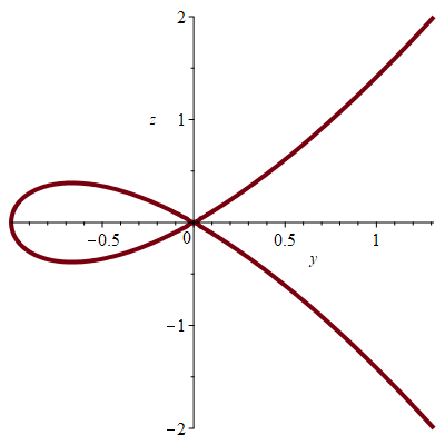
with The corresponding curve is a rational cubic with a double point at the origin (see Fig. 1 left). We apply Algorithm 5 to decompose the points of depending on the existence of non-constant analytic solutions. In Step 1, we get . Let and . In Step 2 we apply Algorithm 5 to the critical points.
For we get two places locally parametrized by and . So, . Since none of the places are order-suitable, we get
For we get the place which is order-suitable. Therefore, we apply Algorithm Reparametrization to . We obtain Thus, .
Therefore, the output of the algorithm is , , which means that: (1) at every point in there exists exactly one non-constant formal power solution that is, indeed, analytic; (2) there is no non-constant analytic solution at ; (3) are the only constant solutions.
Now, to further illustrate the method, we take . A local parametrization at is Applying Algorithm Reparametrization to we get that provides the solution
Example 2.
Consider the following AODE
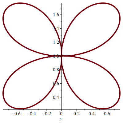
with . The corresponding curve is a rational degree curve with a non-ordinary singularity at (see Fig. 1 right). We apply Algorithm 5. In Step 1, we get where , and .
In Step 2 we apply Algorithm 5 to the critical points.
Let . We get the following four places
So, Observe that only are order-suitable. We apply to them Algorithm Reparametrization. One obtains for , and for , that generate two solutions at , namely (truncated)
Thus, .
Let , where and . We get the place which is not order-suitable. Thus, .
Therefore, the output of Algorithm 5 is , , and , where are as above. Moreover, the constant solutions are . To summarize: (1) At there are two non-constant analytic solutions. (2) At each point in there is exactly 1 non-constant analytic solution. (3) At there is no non-constant analytic solution. (4) At there is no non-constant analytic solution.
In the last part of the section we compare our method with the direct method (see Section 1). The direct method consists in computing the solutions of in . However, finding an upper bound such that every solution of can be extended to a solution of is in general an unsolved problem. This difficulty does no appear in our method as the following example illustrates:
Example 3.
Let us consider the family of irreducible AODEs
where .
Set and . Then .
It is straightforward to see that for each , the differential polynomial is the sum of a linear -combination of terms of the form , with and , and the term .
Moreover, for each , the differential polynomial is a linear -combination of terms of the form , where is a non-constant monomial and . Hence, for and the equations
hold if and only if . However, since
cannot be extended to a formal power series solution. This is exactly the result obtained by Theorem 3.4: for every the curve has a tangent vector parallel to the -axis at and therefore is not a suitable center.
Acknowledgements. The authors are supported by the Spanish Ministerio de Economía y Competitividad, by the European Regional Development Fund (ERDF), under the MTM2017-88796-P. The first author is also supported by the strategic program "Innovatives OÖ 2020" by the Upper Austrian Government and by the Austrian Science Fund (FWF): P 31327-N32.
References
- [1] M.E. Alonso, T. Mora, G. Niesi, and M. Raimondo. Local Parametrization of Space Curves at Singular Points. In Computer Graphics and Mathematics, 61–90. Springer Berlin Heidelberg, 1992.
- [2] J.M. Aroca. Puiseux Solutions of Singular Differential Equations. In Resolution of Singularities, 129–145. Birkhäuser Basel, 2000.
- [3] J.M. Aroca, J. Cano, R. Feng, and X.-S. Gao. Algebraic general solutions of algebraic ordinary differential equations. In Proceedings of the 2005 International Symposium on Symbolic and Algebraic Computation, 29–36. ACM Press, 2005.
- [4] J. Cano. The Newton Polygon Method for Differential Equations. In Proceedings of the 6th International Conference on Computer Algebra and Geometric Algebra with Applications, 18–30. Springer-Verlag, 2005.
- [5] J. Cano and P. Fortuny. The Space of Generalized Formal Power Series Solution of an Ordinary Differential Equations. Astérisque, 323:61–82, 2009.
- [6] E. Casas-Alvero Singularities of Plane Curves. London Mathematical Society Lecture Note Series, Cambridge University Press, 2000.
- [7] J. Denef and L. Lipshitz. Power series solutions of algebraic differential equations. Mathematische Annalen, 267:213–238, 1984.
- [8] D. Duval. Rational puiseux expansion. Compositio Mathematica, 70:119–154, 1989.
- [9] R. Feng and X.-S. Gao. Rational general solutions of algebraic ordinary differential equations. In Proceedings of the 2004 International Symposium on Symbolic and Algebraic Computation, pages 155–162. ACM Press, 2004.
- [10] R. Feng and X.-S. Gao. A polynomial time algorithm for finding rational general solutions of first order autonomous odes. J. Symb. Comput., 41(7):739–762, 2006.
- [11] D.Yu. Grigor’ev and M.F. Singer. Solving Ordinary Differential Equations in Terms of Series with Real Exponents. Transactions of the American Mathematical Society, 327(1):329–351, 1991.
- [12] E. Ince. Ordinary Differential Equations. Dover Books on Mathematics, 1926.
- [13] E.R. Kolchin. Differential Algebra and Algebraic Groups. ACM Press, 1973.
- [14] L.X.C. Ngo and F. Winkler. Rational general solutions of first order non-autonomous parametrizable ODEs. J. Symb. Comput., 45(12):1426–1441, 2010.
- [15] L.X.C. Ngo and F. Winkler. Rational general solutions of planar rational systems of autonomous ODEs. J. Symb. Comput., 46(10):1173–1186, 2011.
- [16] J.F. Ritt. Differential algebra. American Mathematical Society Colloquium, New York, 1950.
- [17] P. Stadelmeyer. On the Computational Complexity of Resolving Curve Singularities and Related Problems. PhD Thesis, Johannes Kepler University Linz, 2000.
- [18] N.T. Vo, G. Grasegger, and F. Winkler. Deciding the Existence of Rational General Solutions for First-Order Algebraic ODEs. J. Symb. Comput., 87:127–139, 2018.
- [19] R.J. Walker. Algebraic curves. Princeton University Press, 1950.