Convection Enhances Magnetic Turbulence in AM CVn Accretion Disks
Abstract
We present the results of local, vertically stratified, radiation magnetohydrodynamic shearing box simulations of magnetorotational instability (MRI) turbulence for a (hydrogen poor) composition applicable to accretion disks in AM CVn type systems. Many of these accreting white dwarf systems are helium analogues of dwarf novae (DNe). We utilize frequency-integrated opacity and equation of state tables appropriate for this regime to accurately portray the relevant thermodynamics. We find bistability of thermal equilibria in the effective temperature, surface mass density plane typically associated with disk instabilities. Along this equilibrium curve (i.e. the S-curve) we find that the stress to thermal pressure ratio varied with peak values of near the tip of the upper branch. Similar to DNe, we found enhancement of near the tip of the upper branch caused by convection; this increase in occurred despite our choice of zero net vertical magnetic flux. Two notable differences we find between DN and AM CVn accretion disk simulations are that AM CVn disks are capable of exhibiting persistent convection in outburst, and ideal MHD is valid throughout quiescence for AM CVns. In contrast, DNe simulations only show intermittent convection, and non-ideal MHD effects are likely important in quiescence. By combining our previous work with these new results, we also find that convective enhancement of the MRI is anticorrelated with mean molecular weight.
Keywords:
accretion, accretion disks; convection; magnetohydrodynamics (MHD); binaries: close; white dwarfsI Introduction
AM Canum Venaticorum type stars (AM CVns) are very short period ( minutes) binary systems consisting of a white dwarf that is accreting from a Roche lobe filling, hydrogen-deficient companion star (often another, lower mass, white dwarf), and can be thought of as helium analogues of cataclysmic variables (see, e.g., Solheim 48 for a review). They are of intrinsic astrophysical interest because they may be sources of helium novae, .Ia supernovae [4], and possibly even type Ia supernovae, as well as being among the strongest known sources of gravitational waves detectable by the future space-based gravitational wave mission LISA (e.g. Nelemans et al. 34). The helium-dominated accretion disks in AM CVns exhibit all the rich phenomenology of hydrogen-dominated accretion disks around white dwarfs, including persistent and outbursting systems, eclipsing systems, superhumps, quasiperiodic oscillations (QPO’s), and broadband noise (e.g. Ramsay et al. 36, Campbell et al. 9, Kupfer et al. 29, Levitan et al. 31). The outbursting systems are generally dominated by superoutbursts, although normal outbursts have also been observed [32].
Ionization driven thermal instability models of outbursting helium accretion disks were first considered by Smak [46] and Cannizzo [10], and more recent models have been developed by Kotko et al. [28] and Cannizzo & Nelemans [11]. As in the standard disk instability models of hydrogen-rich dwarf novae (DNe), these helium dominated models require that the Shakura & Sunyaev [44] parameter be larger in outburst than in quiescence, though the enhancement of need not be as large (possibly as low as a factor of two) as compared to hydrogen accreting systems [28]. The value of in outburst in AM CVn systems appears to be similar to the outburst value of DNe (0.1-0.2), though the observational constraints are currently weaker than in DNe [28, 27].
Explaining the observationally-inferred variation in across the ionization transition has been a challenge. One possibility is that it is related to a high resistivity in the quiescent (and predominantly electrically neutral) state, which would hinder MHD turbulence and reduce there [21]. However, in the outburst state, where ideal MHD should hold, simulations of magnetorotational (MRI, Balbus & Hawley 2, Balbus & Hawley 3) turbulence with no externally imposed vertical magnetic flux typically give time-averaged values of only a few percent.11 1 Questions of numerical convergence still exist for simulations which lack vertical magnetic flux and thermodynamics, e.g. Ryan et al. [39]. Also, there may be a dependence of on box height in local shearing box simulations [45]. Including a net vertical magnetic field can enhance the value of [22, 41, 35], but then this begs the question as to why the outburst values should be so similar across sources.
On the other hand, incorporating the thermodynamics of radiative cooling with realistic opacities and ionizing equation of state in stratified shearing box simulations, [25] found that thermal convection is driven near the ionization transition. This modifies the MRI turbulence so as to enhance in outburst just above the transition to quiescence. Values of there were found to be as high as 0.14, even without the presence of net vertical magnetic flux. This convection-driven enhancement of has since been confirmed using independent numerical codes [43], and was also found just above the hydrogen ionization transition under conditions relevant for the inner regions of protoplanetary disks [24]. In addition to the enhancement of turbulent stresses, convection also alters the character of the MRI “butterfly diagram” dynamo, quenching field reversals because of inward advection of magnetic field with consistent polarity from high altitude [14].
The purpose of this paper is to extend this work on the effects of convection on MRI turbulent stresses to AM CVn disks, which have very different chemical compositions (dominated by helium) to those in DNe (dominated by hydrogen). There are potentially two interesting effects: (1) the existence of two ionization stages of helium may affect the properties of convection, and (2) the high first ionization potential of HeI means that there will be many more free electrons from ionized carbon, nitrogen and oxygen in the quiescent state compared to that in a hydrogen disk, thereby enhancing the electrical conductivity.
The structure of this paper is as follows. In section 2 we briefly review our computational methods, opacities and equation of state, and simulation parameters. In section 3 we discuss our results on the thermal bistability of a helium disk, the MRI turbulent stresses, the properties of convection, and the effects on the MRI dynamo. We discuss the implications of our results in section 4, and summarize our conclusions in section 5.
| Element | Log num frac | Log mass frac | Source |
|---|---|---|---|
| H | -17.1 | -17.7 | AGS05 |
| He | -0.00383 | -0.0157 | BBMP15 |
| C | -2.51 | -2.05 | BBMP15 |
| N | -2.45 | -1.92 | BBMP15 |
| O | -3.67 | -3.08 | BBMP15 |
| Ne | -3.26 | -2.57 | BBMP15 |
| Na | -4.88 | -4.14 | AGS05 |
| Mg | -3.16 | -2.39 | BBMP15 |
| Al | -4.68 | -3.87 | AGS05 |
| Si | -3.54 | -2.71 | AGS05 |
| S | -3.91 | -3.02 | AGS05 |
| Ar | -4.87 | -3.89 | AGS05 |
| Ca | -4.74 | -3.76 | AGS05 |
| Fe | -3.60 | -2.47 | AGS05 |
| Ni | -4.82 | -3.67 | AGS05 |
Note. — Partial list of elemental abundances assumed in this work listed in terms of log10 of number fraction and log10 of mass fraction. Abundances with the source BBMP15 are computed from the mass fraction of the predominant isotope in the accreted matter in Brooks et al. [8]. Abundances from AGS05 are solar abundances as reported by Asplund et al. [1] such that the relative abundance between a given element and the combination of C, N, and O is preserved. For hydrogen we assumed that its number fraction is times that in Asplund et al. [1]. For brevity, elements (other than H) with number fractions below are not listed here but are assumed to be consistent with AGS05.
II Methods
We utilize the zeus code [49, 50] with flux limited diffusion [51] to evolve the equations of radiation magnetohydrodynamics. Our zero net vertical flux shearing-box simulations are based on those presented in Hirose et al. [25], to which we refer the reader for a more thorough discussion of the equations and numerical techniques. The primary difference with that earlier work is composition. Here we assume that hydrogen is negligible and helium is the dominant species (see Table 1), necessitating new equation of state (EOS) and opacity tables.
II.1 Composition
The lack of spectral hydrogen signatures in AM CVns [30, e.g.] signifies a significant departure from solar composition. In addition to this dramatic lack of hydrogen, more subtle differences in the composition of AM CVns result from CNO burning in the prior evolution of the donor star [48]. We therefore use a model of an AM CVn from Brooks et al. [8] as a starting point for our assumed chemical abundances. We examined the freshly accreted material on the surface of the primary white dwarf in this model and used the measured mass fraction of the predominant isotope of several elements as the basis of our composition.
For the remaining elements we assume that the CNO burning which took place in the prior evolutionary states of AM CVns preserves the combined number of C, N and O and leaves the number fraction of most other elements unchanged. For elements not taken from Brooks et al. [8], we assumed that their abundance relative to the combination of C, N and O is identical to solar composition [1]. This means that our assumed composition is consistent with that of a binary star system which started with solar metallicity and evolved into an AM CVn.
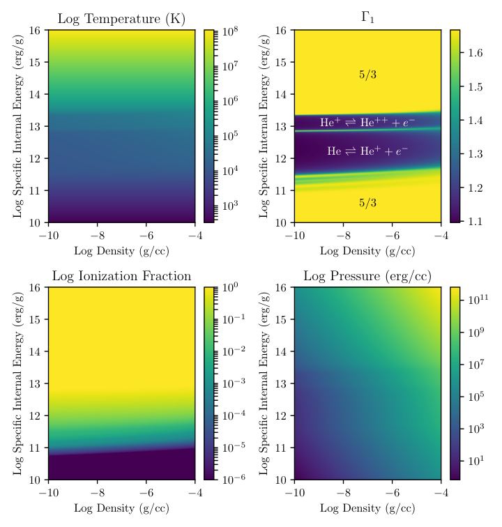
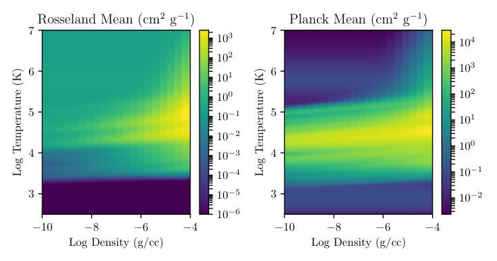
These changes in composition (as well as the orbital frequency ) are the primary differences from the zeus simulations presented in Hirose et al. [25], Hirose [24], Coleman et al. [13], and are only manifest in the EOS and opacity tables. The EOS framework [see Appendix A of 12, for details] used in the shearing box simulations is the same as before, now run with the abundances listed in Table 1, the results of which are shown in Figure 1. We also used this composition to compute our own Rosseland and Planck mean opacities with the latest version of the stellar atmosphere code phoenix [18], with dust explicitly turned off (both in the EOS and opacities). These dust-free tables are shown in Figure 2. We also note that phoenix computes its own EOS which is consistent with that used in our zeus simulations but utilizes a more detailed calculation, required to accurately compute the opacities.
| Run | |||||||||||||||||||||
|---|---|---|---|---|---|---|---|---|---|---|---|---|---|---|---|---|---|---|---|---|---|
| 5.3e3-U0 | 5332 | 40000 | 5287 | 41880 | 4.55e5 | 136106 | 0.016 | 20 | 1.07 | 0.545 | 1.87 | 32 | 64 | 288 | 1 | 2 | 4.5 | 23 | 123 | ||
| 4.4e3-U0 | 4356 | 40000 | 4309 | 40346 | 4.13e5 | 108428 | 0.019 | 19 | 1.02 | 0.542 | 1.87 | 32 | 64 | 288 | 1 | 2 | 4.5 | 44 | 144 | ||
| 1.9e3-U0 | 1915 | 33000 | 1900 | 29203 | 2.66e5 | 61612 | 0.019 | 21 | 0.803 | 0.546 | 1.71 | 32 | 64 | 288 | 1 | 2 | 4.5 | 22 | 122 | ||
| 9.6e2-U0 | 956 | 25000 | 946 | 24082 | 1.98e5 | 37681 | 0.024 | 18 | 0.668 | 0.56 | 1.66 | 32 | 64 | 288 | 1 | 2 | 4.5 | 21 | 121 | ||
| 4.7e2-U0 | 475 | 20000 | 466 | 18655 | 1.34e5 | 24030 | 0.026 | 0.065 | 20 | 0.543 | 0.563 | 1.49 | 32 | 64 | 288 | 1 | 2 | 4.5 | 42 | 142 | |
| 3.7e2-U0 | 375 | 17500 | 366 | 17083 | 1.11e5 | 30662 | 0.030 | 0.228 | 0.301 | 20 | 0.478 | 0.572 | 1.53 | 32 | 64 | 288 | 1 | 2 | 4.5 | 37 | 137 |
| 3.3e2-U2 | 331 | 20000 | 324 | 17749 | 1.14e5 | 19491 | 0.037 | 0.087 | 0.207 | 16 | 0.502 | 0.558 | 1.53 | 32 | 64 | 288 | 1 | 2 | 4.5 | 30 | 130 |
| 2.8e2-U0 | 283 | 20000 | 277 | 16643 | 9.96e4 | 25966 | 0.040 | 0.314 | 0.473 | 16 | 0.486 | 0.529 | 1.4 | 32 | 64 | 288 | 1 | 2 | 4.5 | 45 | 145 |
| 2.3e2-U0 | 232 | 17500 | 226 | 16001 | 9.03e4 | 23640 | 0.047 | 0.395 | 0.639 | 14 | 0.431 | 0.562 | 1.45 | 32 | 64 | 288 | 1 | 2 | 4.5 | 31 | 131 |
| 1.8e2-U1 | 184 | 17000 | 176 | 15366 | 8.12e4 | 19955 | 0.057 | 0.528 | 0.915 | 12 | 0.396 | 0.566 | 1.35 | 32 | 64 | 288 | 1 | 2 | 4.5 | 70 | 170 |
| 1.6e2-U0 | 165 | 17000 | 155 | 14943 | 7.45e4 | 19540 | 0.066 | 0.605 | 1.12 | 10 | 0.385 | 0.549 | 1.25 | 32 | 64 | 288 | 1 | 2 | 4.5 | 80 | 180 |
| 1.6e2-U1 | 156 | 17000 | 149 | 14407 | 6.66e4 | 22414 | 0.070 | 0.724 | 1.37 | 9.83 | 0.379 | 0.514 | 1.22 | 32 | 64 | 288 | 1 | 2 | 4.5 | 79 | 179 |
| 1.5e2-U0 | 153 | 16000 | 145 | 13401 | 5.63e4 | 23304 | 0.073 | 0.804 | 1.71 | 8.73 | 0.274 | 0.62 | 1.24 | 32 | 64 | 288 | 1 | 2 | 4.5 | 33 | 133 |
| 1.4e2-U2 | 137 | 17000 | 133 | 14402 | 6.52e4 | 18694 | 0.079 | 0.726 | 1.6 | 8.83 | 0.364 | 0.532 | 1.09 | 32 | 64 | 288 | 1 | 2 | 4.5 | 30 | 130 |
| 1.3e2-U1 | 128 | 17000 | 120 | 13677 | 5.77e4 | 15918 | 0.091 | 0.747 | 1.8 | 7.57 | 0.355 | 0.485 | 1.02 | 32 | 64 | 288 | 1 | 2 | 4.5 | 80 | 180 |
| 1.2e2-U1 | 118 | 17000 | 110 | 13732 | 5.82e4 | 14032 | 0.098 | 0.715 | 1.85 | 7.16 | 0.343 | 0.514 | 0.992 | 32 | 64 | 288 | 1 | 2 | 4.5 | 80 | 180 |
| 1.1e2-U1 | 109 | 17000 | 101 | 12028 | 4.11e4 | 13080 | 0.113 | 0.768 | 2.25 | 6.03 | 0.331 | 0.388 | 0.82 | 32 | 64 | 288 | 1 | 2 | 4.5 | 80 | 180 |
| 8.9e1-U1 | 89 | 16500 | 85 | 11599 | 3.74e4 | 9517 | 0.146 | 0.751 | 2.82 | 4.76 | 0.264 | 0.453 | 0.883 | 32 | 64 | 288 | 1 | 2 | 4.5 | 32 | 132 |
| 1.9e2-M0 | 192 | 7400 | 180 | 8976 | 2.48e4 | 40760 | 0.047 | 0.884 | 1.36 | 11 | 0.111 | 0.79 | 1.48 | 32 | 64 | 288 | 1 | 2 | 4.5 | 26 | 126 |
| 2.0e2-M0 | 201 | 7400 | 193 | 8676 | 2.40e4 | 40225 | 0.041 | 0.881 | 1.23 | 12 | 0.113 | 0.751 | 1.44 | 32 | 64 | 288 | 1 | 2 | 4.5 | 27 | 127 |
| 2.0e2-M1 | 201 | 7000 | 192 | 8632 | 2.40e4 | 39851 | 0.041 | 0.881 | 1.3 | 12 | 0.11 | 0.773 | 1.44 | 32 | 64 | 288 | 1 | 2 | 4.5 | 33 | 133 |
| 2.1e2-L1 | 210 | 6000 | 202 | 7651 | 2.21e4 | 28935 | 0.028 | 0.827 | 0.906 | 14 | 0.103 | 0.751 | 1.37 | 32 | 64 | 288 | 1 | 2 | 4.5 | 42 | 142 |
| 1.9e2-L1 | 192 | 7000 | 191 | 6129 | 1.90e4 | 9148 | 0.014 | 0.675 | 0.508 | 18 | 0.108 | 0.626 | 1.08 | 32 | 64 | 288 | 1 | 2 | 4.5 | 46 | 146 |
| 1.8e2-L0 | 182 | 16000 | 179 | 6889 | 2.00e4 | 12897 | 0.022 | 0.727 | 0.741 | 15 | 0.122 | 0.582 | 1.04 | 32 | 64 | 288 | 1 | 2 | 4.5 | 62 | 162 |
| 1.7e2-L0 | 173 | 7500 | 172 | 6054 | 1.84e4 | 6225 | 0.016 | 0.591 | 0.455 | 15 | 0.108 | 0.607 | 1.04 | 32 | 64 | 288 | 1 | 2 | 4.5 | 79 | 179 |
| 1.3e2-L0 | 130 | 10000 | 128 | 5017 | 1.36e4 | 865 | 0.016 | 0.208 | 0.156 | 14 | 0.119 | 0.451 | 0.703 | 32 | 64 | 288 | 1 | 2 | 4.5 | 60 | 160 |
| 1.3e2-L1 | 129 | 8700 | 128 | 4390 | 1.05e4 | 599 | 0.012 | 0.243 | 0.141 | 20 | 0.108 | 0.434 | 0.664 | 32 | 64 | 288 | 1 | 2 | 4.5 | 122 | 222 |
| 1.3e2-L2 | 129 | 6000 | 126 | 5169 | 1.49e4 | 1111 | 0.015 | 0.239 | 0.189 | 15 | 0.089 | 0.632 | 1.01 | 32 | 64 | 288 | 1 | 2 | 4.5 | 38 | 138 |
| 1.0e2-L1 | 100 | 5000 | 98 | 4152 | 8.88e3 | 286 | 0.016 | 0.182 | 0.144 | 13 | 0.070 | 0.608 | 0.867 | 32 | 64 | 288 | 1 | 2 | 4.5 | 35 | 135 |
| 7.5e1-L2 | 75 | 3500 | 70 | 3088 | 2.18e3 | 4e-3 | 0.022 | 9.31 | 0.041 | 0.606 | N/A | 32 | 64 | 288 | 1 | 2 | 4.5 | 80 | 180 |
Note. — Each row corresponds to the parameters of a simulation where the name of the run is specified in the first column. The second to last character of a run name denotes the branch which the simulation settled to: “U” for upper, “M” for middle, and “L” for lower. Times () are listed in orbital periods, all other numbers are given in cgs units. Zero in the subscript denotes initial conditions. All other values have been averaged over the time interval from to . is the surface mass density, are the effective and central temperatures, is the total optical depth integrated between the vertical bounds of the simulation, is the ratio of volume and time-averaged stressed to volume and time-averaged thermal pressure, and are estimators of convective strength and are given by Eqns. 3 and 4 respectively, is the thermal time, is the simulation length unit, is the pressure scale-height, is the photosphere height, are the number of cells in the coordinate directions, and are the lengths of the simulation domain.

II.2 Parameters
One of the most important and fundamental parameters for a shearing box is its orbital frequency
| (1) |
with cm and as the assumed radius and mass of the white dwarf primary. We take rad s-1 for all the simulations presented in this work. The surface mass density is also important, as it determines the types of possible thermal equilibria. Additionally, the net vertical magnetic flux is also an inherently interesting parameter [40, see e.g.], however we keep this zero to minimize our parameter space and to explore enhancements of where it typically takes its lowest value. Neglecting the usually small mass loss through our vertical outflow boundary conditions, these three parameters are conserved through the evolution of a shearing box simulation.
In addition to these conserved parameters the choice of an initial effective temperature is necessary to establish initial conditions based on simplistic hydrostatic and thermal equilibrium [see Section 2.4 of 25, for more details]. As the simulation evolves the MRI sets in and develops turbulence, typically within 10 orbits. This turbulence naturally results in dissipation occurring throughout the disk, which responds by either heating or cooling until a quasi-steady state is achieved, which may be significantly far from the assumed initial condition. The parameters which define these initial conditions along with several time averaged quantities of our various simulations are shown in Table 2.
III Results
To discuss our results, it is useful to define the following quantities related to some fluid variable : the horizontal average of this quantity, a one orbit temporally smoothed quantity, the temporal mean, and the mean midplane value. These are defined respectively by
| (2a) | ||||
| (2b) | ||||
| (2c) | ||||
| (2d) | ||||
Here , , and are the radial, azimuthal and vertical extents of the simulation domain, respectively, and , are the endpoints used for temporal integration (listed in Table 2).
III.1 Thermal Equilibria
An essential aspect of analyzing disk instabilities is understanding the conditions leading to thermal equilibrium. It is common to depict the thermal equilibria of a local patch of an accretion disk as a curve in the plane of surface mass density and effective temperature . Near an ionization transition (or other instabilities), this curve typically has a distinctive shape leading to the name S-curve. The thermal equilibria resulting from shearing box simulations such as ours (see Figure 3) are often missing most, if not all, of the middle branch which gives the curve its distinctive S shape. This is because the negative slope of this region of the curve indicates that these equilibria are formally unstable. However, numerical effects can lead to additional stability in this region, resulting in simulations being erroneously attracted to this branch (see e.g. Section 5.2 of Jiang et al. 26).
III.2 Enhancement of
As can be seen in Figure 3, our measured values vary along the S-curve reaching a maximum of near the tip of the upper branch, with low values of a few percent high up on the upper (outburst) branch and all along the lower (quiescent) branch. This gives a variation of that is relatively large (a factor of ), similar to that inferred for DNe [47, 27, 25, 43, e.g.], and consistent with modeling of AM CVn lightcurves, but notably higher than the inferred lower limit of the ratio of minimum and maximum values [28].
Following Hirose et al. [25], Hirose [24], we define the quantities as a means to estimate the fraction of vertical energy transport which is done by advection,
| (3) |
and an estimate of the Mach number of advective eddies,
| (4) |
where is the gas internal energy density, is the radiation energy density, is the vertical velocity, is the thermal pressure (gas plus radiation), and is the total energy flux in the vertical direction, including Poynting and radiation diffusion flux.
We first presented the results of convection enhancing in Hirose et al. [25], where we showed that was correlated with (see orange points in the left frame of Figure 4). However, Hirose [24] noted that with additional data it became clear that was more correlated with , and Scepi et al. [43] have also noted that is not well correlated with . Here we further confirm these results in Figure 4 where we present the data from this work along with those from Hirose et al. [25], Hirose [24], and Coleman et al. [13]. With these data it seems clear that convection22 2 We have yet to identify a way to conclusively distinguish convection from advection, although it is clear that our simulations are convectively unstable because they exhibit a negative vertical entropy gradient. dominated energy transport through the disk is not sufficient to enhance . The convection must not be slow (i.e. ) in order for it to enhance .
From Equations 3 and 4 it is clear that and are closely related. By incorporating the Shakura & Sunyaev [44] prescription
| (5) |
where is the sound speed, one can write the following relation33 3 We thank the anonymous referee for pointing out this relation to us and for coming up with the concept of Fig. 5.:
| (6) |
In Fig. 5 we show that this describes our data reasonably well. However, the spread in the relation increases with , indicating that as convection saturates (i.e. as ) the connection between and breaks down. This may be related to the fact is not fixed in our simulations and the same physics (i.e. ionization transitions) which leads to high also causes to vary. For instance, in simulation 8.9e1-U1 and the midplane value of varies from . This combined with the fact that the correlations between and (Fig. 4), and and (Fig. 5) worsen at roughly the same value of suggests that is the more relevant physical quantity to be compared with .
The correlation we find between and is consistent with our hypothesis [25] that this enhancement of is caused by convection advecting magnetic fields and seeding the MRI with vertical fields. The axisymmetric MRI then feeds off of this and generates stronger magnetic turbulence resulting in an enhancement in . However, we stress that the mean turbulent motion (i.e. the RMS value of ) is times the speed of the convective eddies (), making identifying the effect of convection on the MRI challenging. Despite being small compared to the mean vertical motion, we have demonstrated in our previous work that convective eddies are capable of advecting strong magnetic fields vertically (see Coleman et al. 14, in particular Figures 5 and 6).
We also note there are many helium disk simulations (purple points) and Hirose [24] simulation (blue points) in the bottom right corner of the left panel of Fig. 4. These points are almost all from the lower or middle branches, indicating that convection occurring at temperatures lower than the corresponding ionization transition is inefficient at enhancing . Both hydrogen and helium simulations occupy this parameter space, implying that low temperature convection gives low for relatively high regardless of composition.
Additionally, the helium simulations have systematically lower values for compared to hydrogen simulations from the same branch with comparable or . This seems to be related to the increased mean molecular weight as scaling by (as was done in Fig. 4) hides this effect and increases the correlation at , but worsens the correlation when convection is not present. It is not clear why is related to the convective enhancement of the MRI, however is known to be related to the efficiency of convection within the context of mixing-length theory [6, 33, e.g.] suggesting that the two should be related.
III.3 Persistent Convection
One of the most noticeable differences compared to our previous work on DN simulations [25, 13, 14] is that our simulations of AM CVn disks exhibit persistent convection. With the exception of one simulation (ws0837 from Hirose 24), all of our previous simulations exhibiting convection did so intermittently. Scepi et al. [43] also found their DNe simulations to exhibit intermittent convection. However, several of our AM CVn simulations exhibit persistent convection. In Fig. 6 we show the evolution of the midplane Rosseland mean opacity and adiabatic index for three simulations. These simulations are representative of the trend we find between persistence of convection and location in the opacity curve. Simulations which exhibit few to zero transitions out of epochs dominated by convective energy transport stay between the two maxima in Rosseland mean opacity resulting from the two ionizations of helium. This implies that the concave nature of the He opacity curve is what stabilizes the convective transport within the disk.
The simulation 2.3e2-U0 (green curves in Fig. 6 and third panel in Figs. 7 and 8) exhibits intermittent convection similar to what we presented in Section 3.4 of Hirose et al. [25]. We originally described this behavior as a limit cycle, which we summarize here. Simulations towards the tip of the upper branch often switch between epochs where energy transport is dominated by radiative diffusion and convection. During convective epochs, turbulent stress and dissipation is increased causing the disk to heat. This heating combined with large and negative values of makes it easier for photons to escape and the disk transitions to a radiative epoch. This transition is accompanied by a decline in turbulent heating, causing the disk to be slightly too effective at removing heat. This leads to cooling and higher opacities which then initiates convection, thereby completing the limit cycle.
From this description it is clear that the negative values of on the upper branch of the S-curve are fundamental to driving this limit cycle. The double peaked nature of the He opacity curve ensures that the opacity increases regardless of heating/cooling, preventing the disk from losing optical depth, thereby preventing a transition to radiative epochs. In other words, the increase in opacity in both directions always requires superadiabatic temperature gradients to get the heat out.
This finding also shows that the enhancement of does not require convection to be intermittent, causing our emphasis on the convective limit cycle in Section 3.4 of Hirose et al. [25] to be slightly misleading. While this limit-cycle is interesting and has given us some insight into the dynamo [14], it does not seem to play a key role in enhancing . This can be visualized44 4 We thank the referee for encouraging us to add this plot. in Fig. 7 which shows that and for the duration of simulation 8.9e1-U1. Although, this need not be the case as 1.3e2-U1 maintains but has dips in which seem to lag dips in by orbits. Finally, 2.3e2-U0 shows intermittent convection similar to that in Hirose et al. [25] where dips in and appear to be correlated.

III.4 Quenching of Dynamo Reversals
In the simulations presented here, we found that convection modifies the standard dynamo found in accretion disk simulations [7, 16, see e.g.] by quenching magnetic field reversals (see Figure 8). We discussed this particular phenomenon in depth in Coleman et al. [14]. We show the dynamo behavior of four of our simulations in Figure 8 with persistent, nearly-persistent, intermittent, and no convection.
Our simulations with persistent convection offer a new way to examine this quenching over longer timescales. For the case of our persistent simulations, the dynamo maintains a constant sign of for long durations. In Coleman et al. [14] we hypothesized that the polarity of the magnetic fields at the beginning of a convective epoch is held fixed until the simulation becomes convectively stable. This is consistent with the fact that our persistently convective simulations tend to maintain the same parity and sign of as that of our initial conditions55 5 This indicates that to perform a proper dynamo study of convective accretion disks, it is necessary to examine multiple initial field configurations. However, this is beyond the scope of this work.. However, we do see some magnetic field reversals in persistently convective simulations which seem uncorrelated to . In these cases there is evidence that dips in are associated with field reversals while (see marked times in Figs. 7 and 8 for simulation 1.3e2-U1).
III.5 Validity of Ideal MHD
For DNe (with a hydrogen dominated composition) it is unclear how well the plasma within the disk can be described by MHD [21, see e.g.]. As we discussed in Coleman et al. [13], post-processing of our DNe simulations (which assume ideal MHD) suggest that non-ideal MHD effects are important along the entire quiescent branch. In particular we found that Ohmic dissipation is important, the Hall term may need to be taken into consideration, and that ambipolar-diffusion was negligible. Scepi et al. [43] incorporated Ohmic dissipation directly in their simulations, neglecting the Hall term, and found that the transition from ideal to non-ideal MHD occurred below the tip of quiescent branch. They estimated that the Hall term is an order of magnitude smaller than Ohmic dissipation, leading them to conclude that only Ohmic dissipation is important. In contrast to these results for DNe, we find here that ideal MHD should always be applicable to AM CVns. The reason for this is that the abundant elements C, N, and O remain ionized in the quiescent state, and are therefore copious sources of free electrons.
To estimate the validity of ideal MHD we computed the magnetic Reynolds number (Rem) following Fleming et al. [19] and the Hall Lundquist number () following Scepi et al. [43] assuming thermal ionization from our AM CVn simulation data (see Fig 9).
| (7) |
where cm2 s-1 is the Ohmic diffusivity coefficient [5], and are the number density of the neutrals and electrons respectively.
| (8) |
where is mass density, is the elementary charge, is the pressure scale height, and is the speed of light. For our coldest optically thick simulation both of these numbers are within the photosphere. This combined with previous studies of non-ideal MHD [23, 42, 43, e.g.] suggests that ideal MHD is a good approximation for AM CVns, even throughout quiescence.

IV Discussion
IV.1 Observational Constraints
| System Name | (min) | (min) | Source | |||
|---|---|---|---|---|---|---|
| Persistent High State | ||||||
| ES Cet | 10.3 | 4.79 | 2 | 4 | Espaillat et al. [17] | |
| AM CVn | 17.1 | 7.95 | 5.6 | 9.3 | Roelofs et al. [38] | |
| KIC 004547333 (SDSS J1908) | 18.1 | 8.41 | 3.5 | 8.5 | Fontaine et al. [20] | |
| HP Lib | 18.4 | 8.55 | 0.81 | 2.2 | Roelofs et al. [38] | |
| Outbursting | ||||||
| CR Boo | 24.5 | 11.4 | 0.38 | 1.2 | Roelofs et al. [38] | |
| KL Dra | 25 | 11.6 | 0.47 | 1.57 | Ramsay et al. [37] | |
| V803 Cen | 26.6 | 12.4 | 0.57 | 1.6 | Roelofs et al. [38] | |
| Persistent Quiescence | ||||||
| GP Com | 46.5 | 21.6 | 0.0036 | Roelofs et al. [38] | ||
Note. — is the orbital period of the binary, is the estimated orbital period at the outer disk edge (see Eqn. 14), and are the lower and upper bounds on the mass transfer rate respectively. is the estimated mass transfer rate; values denoted by an asterisk are simply taken to be the geometric mean of the upper and lower bounds.
Based on our S-curve for rad s-1 (Figure 3) our data suggest that the critical effective temperatures K and K at the annulus we simulated. For the discussion that follows we assume that torques on the disk by the binary companion and the accreting white dwarf and other edge effects are negligible, therefore
| (9) |
where is the orbital period for a given annulus in the accretion disk. This implies our simulated annulus is unstable to mass accretion rates between and yr-1. To understand instability criteria for normal AM CVn outbursts we need and for the whole disk. Since our data is limited to one annulus we assume
| (10) |
based on the scalings from Eqns. 7 and 9 of Kotko et al. [28]. From this we derive the following limiting mass transfer rates as a function of orbital period within the accretion disk:
| (11) | ||||
| (12) |
We stress that these limits are for a local instability at a given annulus (in terms of its orbital period) within an accretion disk. For a global instability (i.e. an outburst) to occur, presumably a significant range of annuli must be unstable. In other words instability at a single annulus is a necessary, but not sufficient condition for the onset of outbursts.
To compare these results to observed AM CVns we need estimates for the mass transfer rate and outer disk edge. The former can be inferred from parallaxes and luminosities [38, see e.g.]. As for the later, the outer disk edge () can be estimated as [52]
| (13) |
where is the semi-major axis of the binary and is the mass ratio. Assuming that is small gives us a rough estimate of the orbital period of the outer disk edge () in terms of the orbital period of the binary ():
| (14) |
We compiled observational data for several AM CVns in Table 3 and plotted this data along with our critical mass transfer rates in Fig. 10. This shows that our simulations are consistent with observed AM CVns.
IV.1.1 Lightcurves
Another observational aspect that could be tested is the appearance of outburst lightcurves, as we did for DNe in Coleman et al. [13]. In that work all of our lightcurves based on our MHD simulations had peculiar zig-zagging decays from outburst called reflares, which are not observed in standard DNe. Here we speculate on how the issue of reflares might change for the AM CVn case. However, we leave the computation of outburst lightcurves for another paper.
Both the variation of alpha and the locations of the ends of the upper and lower branches play significant roles in shaping the lightcurve generated by the associated disk instability, as noted in our previous work in Coleman et al. [13]. The contrast in the critical values (ends of the branches) and the variation of is comparable to what we found for the DN case, suggesting that reflares may be an issue for utilizing the disk instability model (DIM) to generate light curves for AM CVns.
Despite this, there are some aspects of our AM CVn simulations which could alleviate the reflare problem. We note that for our DN work, the physical assumptions (e.g. high optical depth, ideal MHD) made in both our zeus simulations and DIM models start to break down at the end of the lower branch, and these two methods also disagree on the end of the lower branch. If these issues are the cause of the reflares found in Coleman et al. [13], then re-performing these calculations for the AM CVn case could result in lightcurves free of reflares, as both ideal MHD and high optical depths are good approximations. Also, because the convection towards the end of the upper branch is persistent (instead of intermittent) for AM CVns, using temporal means of the simulations as inputs for the DIM may result in better agreement between the two.
Additionally, observations of lightcurves for AM CVns pale in comparison to DNe. This is a reflection of the scarcity of these sources more than anything else; there are only known AM CVns with of them outbursting with normal outburst duration day [28, 31]. In contrast, the Catalina Real-time Transient Survey alone has over 700 classified DNe [15]. This makes the observational constraints of AM CVn normal light curves, including lack of reflares, much weaker. Therefore the addition of high cadence high quality lightcurves of normal outbursts in AM CVns would enable better tests of accretion disk theory.
IV.2 Compositional Dependence
We found that the convective enhancement of the MRI (measured through ) is weaker for higher mean molecular weight at a given or ; this is demonstrated in Fig. 4 by scaling by . As discussed in Section III.3 we also found the stability/persistence of convection is significantly different between disks which are H dominated (e.g. DNe) and He dominated (e.g. AM CVns), with convection in He disks exhibiting persistent convection. Finally, we found that the compositional difference between DNe and AM CVns results in significantly different conductivities in quiescence for these systems (see Section III.5). This is because even when He is neutral the disk is still sufficiently hot for C, N, and O to be singly ionized enabling high conductivity throughout AM CVn quiescence, impling that the difference in between the hot and cold states cannot be explained by varying conductivities for AM CVns. These remarkable differences caused by composition are only identifiable through proper treatments of thermodynamics and radiation. While it remains to be seen how accurately our simulations represent nature, it is clear that this microphysics significantly affects the outcome and it would be naïve to believe that nature is indifferent to this.
V Conclusions
In this paper we presented radiation-MHD stratified shearing-box simulation of AM CVn accretion disks. We found many similarities to our previous work on H dominated DNe accretion disks [25, e.g.]. In particular we found a similar S-curve (Fig. 3) and trend in the variation of , with enhancement only occurring near the tip of the upper branch, with peak values at the tip of . This suggests that normal outbursts in AM CVns are very similar to those found in DNe. Likewise we also found that this enhancement of is caused by convection which only manifests itself near the tip of the upper branch due the sharp temperature dependence of the EOS and opacities (see Figs. 1, 2, and 6). Additionally, this convection acts to quench magnetic field reversals (see Fig. 8) as we previously found in Coleman et al. [14].
While these two types of accretion disks have many similarities, we noted some significant differences between our AM CVn and DN simulations: 1) Convective enhancement of and the mean molecular weight are anticorrelated. 2) AM CVn simulations which lie between the two He opacity peaks exhibit persistent convection, while the convection found in H dominated disks is almost always intermittent. 3) The high ionization temperature of neutral He enables C, N, and O to be ionized even when He is neutral, leading to non-ideal MHD terms being negligibly small throughout quiescence in AM CVns. Contrastingly, non-ideal MHD terms are suspected to become important for DNe somewhere on the quiescent branch [21, 13, see e.g.]. The uncertainty of where this transition occurs can be highlighted by the fact that Hirose et al. [25] and Scepi et al. [43] recover different endpoints for the lower branch66 6 Although it should be noted that these works perform their analysis at slightly different , which is known to effect the S-curve., with Hirose et al. 25 reporting lower and higher for the tip of the lower branch. This causes them to disagree on where the transition away from ideal MHD lies. However, the value of where Scepi et al. [43] find non-ideal effects become important is consistent with the results of Hirose et al. [25] and their follow-up work Coleman et al. [13].
Acknowledgements
We thank the anonymous referee for a constructive report that led to significant improvements in this paper. We also thank Jared Brooks, Evan Bauer, Paul Groot, Iwona Kotko, and Jean-Pierre Lasota for their useful discussions and insight generated from their work. This research was supported by the United States National Science Foundation (NSF) under grant AST-1412417. Several of the above discussions were facilitated by a KITP program and so this research was supported in part by the NSF Grant PHY-1125915. This work used the Extreme Science and Engineering Discovery Environment (XSEDE), which is supported by National Science Foundation grant number ACI-1548562. Specifically, we utilized the Comet cluster at the San Diego Supercomputer Center at UC San Diego through allocation TG-AST160025. The EOS and opacity calculations were partly carried out on the Cray XT4 at CfCA, National Astronomical Observatory of Japan, and on SR16000 at YITP in Kyoto University. MC gratefully acknowledges support from the Institute for Advanced Study, NSF via grant AST-1515763, and NASA via grant 14-ATP14-0059. SH was supported by Japan JSPS KAKENHI 15K05040 and the joint research project of ILE, Osaka University.
References
- [1] Asplund, M., Grevesse, N., & Sauval, A. J. 2005, in Astronomical Society of the Pacific Conference Series, Vol. 336, Cosmic Abundances as Records of Stellar Evolution and Nucleosynthesis, ed. T. G. Barnes, III & F. N. Bash, 25
- [2] Balbus, S. A., & Hawley, J. F. 1991, ApJ, 376, 214
- [3] —. 1998, Reviews of Modern Physics, 70, 1
- [4] Bildsten, L., Shen, K. J., Weinberg, N. N., & Nelemans, G. 2007, ApJ, 662, L95
- [5] Blaes, O. M., & Balbus, S. A. 1994, ApJ, 421, 163
- [6] Böhm-Vitense, E. 1958, ZAp, 46, 108
- [7] Brandenburg, A., Nordlund, A., Stein, R. F., & Torkelsson, U. 1995, ApJ, 446, 741
- [8] Brooks, J., Bildsten, L., Marchant, P., & Paxton, B. 2015, ApJ, 807, 74
- [9] Campbell, H. C., Marsh, T. R., Fraser, M., et al. 2015, MNRAS, 452, 1060
- [10] Cannizzo, J. K. 1984, Nature, 311, 443
- [11] Cannizzo, J. K., & Nelemans, G. 2015, ApJ, 803, 19
- [12] Coleman, M. S. B. 2017, PhD thesis, University of California Santa Barbara. https://search.proquest.com/docview/1937891540
- [13] Coleman, M. S. B., Kotko, I., Blaes, O., Lasota, J.-P., & Hirose, S. 2016, MNRAS, 462, 3710
- [14] Coleman, M. S. B., Yerger, E., Blaes, O., Salvesen, G., & Hirose, S. 2017, MNRAS, 467, 2625
- [15] Coppejans, D. L., Körding, E. G., Knigge, C., et al. 2016, MNRAS, 456, 4441
- [16] Davis, S. W., Stone, J. M., & Pessah, M. E. 2010, ApJ, 713, 52
- [17] Espaillat, C., Patterson, J., Warner, B., & Woudt, P. 2005, PASP, 117, 189
- [18] Ferguson, J. W., Alexander, D. R., Allard, F., et al. 2005, ApJ, 623, 585
- [19] Fleming, T. P., Stone, J. M., & Hawley, J. F. 2000, ApJ, 530, 464
- [20] Fontaine, G., Brassard, P., Green, E. M., et al. 2011, ApJ, 726, 92
- [21] Gammie, C. F., & Menou, K. 1998, ApJ, 492, L75
- [22] Hawley, J. F., Gammie, C. F., & Balbus, S. A. 1995, ApJ, 440, 742
- [23] —. 1996, ApJ, 464, 690
- [24] Hirose, S. 2015, MNRAS, 448, 3105
- [25] Hirose, S., Blaes, O., Krolik, J. H., Coleman, M. S. B., & Sano, T. 2014, ApJ, 787, 1
- [26] Jiang, Y.-F., Stone, J. M., & Davis, S. W. 2013, ApJ, 778, 65
- [27] Kotko, I., & Lasota, J.-P. 2012, A&A, 545, A115
- [28] Kotko, I., Lasota, J.-P., Dubus, G., & Hameury, J.-M. 2012, A&A, 544, A13
- [29] Kupfer, T., Groot, P. J., Bloemen, S., et al. 2015a, MNRAS, 453, 483
- [30] —. 2015b, MNRAS, 453, 483
- [31] Levitan, D., Groot, P. J., Prince, T. A., et al. 2015, MNRAS, 446, 391
- [32] Levitan, D., Fulton, B. J., Groot, P. J., et al. 2011, ApJ, 739, 68
- [33] Ludwig, H.-G., Allard, F., & Hauschildt, P. H. 2002, A&A, 395, 99
- [34] Nelemans, G., Yungelson, L. R., & Portegies Zwart, S. F. 2004, MNRAS, 349, 181
- [35] Pessah, M. E., Chan, C.-k., & Psaltis, D. 2007, ApJ, 668, L51
- [36] Ramsay, G., Barclay, T., Steeghs, D., et al. 2012, MNRAS, 419, 2836
- [37] Ramsay, G., Kotko, I., Barclay, T., et al. 2010, MNRAS, 407, 1819
- [38] Roelofs, G. H. A., Groot, P. J., Benedict, G. F., et al. 2007, ApJ, 666, 1174
- [39] Ryan, B. R., Gammie, C. F., Fromang, S., & Kestener, P. 2017, ApJ, 840, 6
- [40] Salvesen, G., Simon, J. B., Armitage, P. J., & Begelman, M. C. 2016, MNRAS, 457, 857
- [41] Sano, T., Inutsuka, S.-i., Turner, N. J., & Stone, J. M. 2004, ApJ, 605, 321
- [42] Sano, T., & Stone, J. M. 2002, ApJ, 577, 534
- [43] Scepi, N., Lesur, G., Dubus, G., & Flock, M. 2018, A&A, 609, A77
- [44] Shakura, N. I., & Sunyaev, R. A. 1973, A&A, 24, 337
- [45] Shi, J.-M., Stone, J. M., & Huang, C. X. 2016, MNRAS, 456, 2273
- [46] Smak, J. 1983, Acta Astron., 33, 333
- [47] —. 1999, Acta Astron., 49, 391
- [48] Solheim, J.-E. 2010, PASP, 122, 1133
- [49] Stone, J. M., & Norman, M. L. 1992a, ApJS, 80, 753
- [50] —. 1992b, ApJS, 80, 791
- [51] Turner, N. J., & Stone, J. M. 2001, ApJS, 135, 95
- [52] Warner, B. 2003, Cataclysmic Variable Stars, 592, doi:10.1017/CB09780511586491