Information-thermodynamic characterization of stochastic Boolean networks

Shun Otsubo Affiliation: Department of Applied Physics, The University of Tokyo, 7-3-1 Hongo, Bunkyo-ku, Tokyo 113-8656, Japan Takahiro Sagawa Affiliation: Department of Applied Physics, The University of Tokyo, 7-3-1 Hongo, Bunkyo-ku, Tokyo 113-8656, Japan

August 24, 2026

Abstract

Recent progress in experimental techniques has enabled us to quantitatively study stochastic and flexible behavior of biological systems. For example, gene regulatory networks perform stochastic information processing and their functionalities have been extensively studied. In gene regulatory networks, there are specific subgraphs called network motifs that occur at frequencies much higher than those found in randomized networks. Further understanding of the designing principle of such networks is highly desirable. In a different context, information thermodynamics has been developed as a theoretical framework that generalizes non-equilibrium thermodynamics to stochastically fluctuating systems with information. Here we systematically characterize gene regulatory networks on the basis of information thermodynamics. We model three-node gene regulatory patterns by a stochastic Boolean model, which receive one or two input signals that carry external information. For the case of a single input, we found that all the three-node patterns are classified into four types by using information-thermodynamic quantities such as dissipation and mutual information, and reveal to which type each network motif belongs. Next, we consider the case where there are two inputs, and evaluate the capacity of logical operation of the three-node patterns by using tripartite mutual information, and argue the reason why patterns with fewer edges are preferred in natural selection. This result might also explain the difference of the occurrence frequencies among different types of feedforward-loop network motifs.

I Introduction

In the recent development of single-cell technologies, quantitative biology has attracted much attention [1], where one of the hot topics is the study of network motifs in gene regulatory networks [2, 3, 4, 5]. Complex gene regulatory networks are constituted of specific subgraphs called network motifs that occur much more frequently than those in random networks.
In this study, we focus on three-node patterns, which can be regarded as building blocks of gene regulatory networks. We list all the three-node network motifs in Fig. 1 (see the caption for the details). Many studies have investigated the function of network motifs in order to reveal the reason why such specific patterns are preferred compared to the others in natural selection [2, 6, 7, 5, 8, 9, 10, 11, 12]. Interestingly, they are commonly found in gene regulatory networks across species, including E.coli, yeast, mouse and human [4, 7, 5, 13, 14]. This suggests that there is a guiding principle for the network formation, while we have not yet clearly understood which properties distinguish network motifs from the others. We note that there are few researches that characterize network patterns exhaustively focusing on information quantities and thermodynamic cost, while some studies systematically investigated three-node patterns [15] based on the control theory perspective (e.g., a stability analysis).

Refer to caption — Figure 1: Gene regulatory network motifs: We list all the three-node network motifs. We refer to these patterns as network motifs, because according to previous studies, they occur statistically significantly in gene regulatory networks than those in random networks. This listing and the following explanation are based on Ref. [7, 5]. A node represents a gene, and an arrow represents regulation between genes. Black arrows represent activation, and white ones represent inhibition. There are eight types of FFLs, which are categorized into two groups according to whether the signs of the two regulation paths from the top to the bottom node are equivalent or not. It is known that the CFFLs can act as low-pass filters and the IFFLs show adaptive behavior. There are a lot of sign variations in the PFBL network motifs (see Fig. 19), thus we list two of them above (and the others are just the sign variations of these two patterns). The PFBL network motifs are known to have two functions. One is keeping their states static, and the other is having their states bistable (see Appendix D.4). In this study, we refer to a positive feedback loop that are categorized into network motif as PFBLs.

In statistical physics, information thermodynamics has been developed in the last decade on the basis of stochastic thermodynamics [16, 17, 18], which clarifies the relation between thermodynamic quantities and information [19, 20, 21, 22, 23, 24, 25, 26]. Since biological systems, especially cells, can be regarded as information processing systems that operate by consuming energy sources such as ATP molecules, information thermodynamics can be applied to biological systems. In fact, several studies have revealed information-thermodynamic structure in, for example, sensory adaptation of E. coli chemotaxis [27, 28, 29, 30, 31, 32]. However, biochemical reaction networks including gene regulatory networks are yet to be further investigated.
Here we systematically characterize gene regulatory network patterns on the basis of information thermodynamics. We calculate information-thermodynamic quantities such as the efficiency of information propagation and energetic dissipation to characterize all the possible three-node patterns (704 patterns), by using a stochastic Boolean model. Since the stochastic Boolean model is a coarse-grained model, the dissipation obtained here is a lower bound of the real entropy production [33, 34]. First, we consider the case where there is a single input signal to a three-node pattern, and reveal that all the patterns can be classified into four types. These four types are characterized as dissipative, static, informative, and adaptive. The coherent feedforward loop (CFFL) network motifs belong to the informative type, and the incoherent feedforward loop (IFFL) network motifs belong to the adaptive type. The positive feedback loop (PFBL) network motifs belong to the static type or informative type, and no network motifs are categorized into the dissipative type.
We next consider the case where there are two input signals to a three-node pattern. We evaluate the capacity of logical operation on these two inputs by using tripartite mutual information, and reveal that the FFLs outperform the others. This result clearly accounts for network patterns that occur frequently in gene regulatory networks. It could also be a reasonable explanation for the fundamental difference of the occurrence frequencies among different types of FFLs [8, 9].
These results indicate that gene regulatory networks are efficient in terms of information propagation and thermodynamics. The key features of our work are the following. First, information thermodynamics enables us to quantify dissipation of only a three-node pattern in a large-scale network, by taking the effect of the correlation as the learning rate. We do not make the assumption of an isolation of a three-node pattern from a network, which is the very benefit of using information thermodynamics. Second, we found that tripartite mutual information is useful to characterize the capacity of logical operation performed by three-node patterns. Our approach with these features can be applied to wide range of networks including both artificial and biochemical ones.
This paper is organized as follows. In Sec. II, we introduce the stochastic Boolean model and describe the setup of this study. We also review the fundamental concepts in information thermodynamics. In Sec. III, we show our main results. In the first part, we consider the case of a single input and classify all the three-node patterns on the basis of information-thermodynamic quantities. In the second part, we consider the case of two inputs and calculate tripartite mutual information to evaluate the capacity of logical operation. In Sec. IV, we make concluding remarks.

II Setup

In this section, we formulate the setup of this study with a stochastic Boolean model. We also briefly review information thermodynamics.

II.1 Stochastic Boolean model

We first discuss the general properties of gene regulation. In this study, we restrict ourselves to transcriptional regulation, while post-transcriptional regulation is also important [35, 36, 37]. A gene regulatory network is represented by a graph, whose nodes and directed edges represent genes and their regulation, respectively. In this study, we focus on three-node patterns which are elementary components of gene regulatory networks.
A three-node pattern receives one or two input signals as shown in Fig. 2 and Fig. 5, and passes information to the next nodes by processing the signals. In the single-input case a pattern just propagates information, while in the two-input case it performs logical operation.
There are two types of regulation: activation and inhibition. Therefore, there are $3^{6}-8\cdot 3-1=704$ patterns in total if we exclude auto-regulation.
We next formulate the stochastic Boolean model [38, 39, 40]. Suppose in general that there are $N$ nodes, and each node $X^{i}_{t}~(i=1,2,\cdots,N)$ takes 0 or 1 at continuous time $t$ . The value of each node represents whether the number of proteins produced by the gene exceeds a threshold value as shown in Fig. 2. Inhibitory regulation is described by the NOT gate. Regulation by multiple nodes is expressed by a logic function such as AND or OR, and the state of a node $i$ is determined by the value of a regulatory function $f^{i}(X^{j}_{t},X^{k}_{t},...)$ with nodes $j,k...$ regulating the node $i$ . In this study, for the sake of simplicity, we assume each regulatory function as the AND gate, which is considered as one of the major regulatory functions in gene regulatory networks. (The AND and OR gates are considered to be the two major regulatory functions [7]. The relation between our results and the assumption of regulatory functions is discussed in Appendix B.) For example, in the case of Fig. 2, regulatory functions take the following expressions: $f^{X}(S_{t})=S_{t},~f^{Y}(X_{t})={\rm NOT}(X_{t})$ and $f^{Z}(X_{t},Y_{t})={\rm AND}(X_{t},Y_{t})$ .
In real gene regulatory networks, the state of a gene $i$ (i.e., $X_{t}^{i}=0,1$ ) changes stochastically. Therefore, the time evolution of a gene expression is described by the master equation with the following transition rates:

			(1)
			(2)

Here,γ_i $isatransitionrateand$ e_i $isthereversetransitionratio.Thetransitionmatrixofthemasterequationisconstructedbytheabovetransitionrates(seeAppendix\ref{sec: app1}foranexample)$ SuchBooleanmodelshavebeenusedtodescribethebehaviorofgeneregulatorynetworkscomposedofmorethantwonodes[41, 42, 39, 43, 44, 45].Strictlyspeaking,aBooleanmodelmightbesomewhatinaccuratefordescribingoscillationsinducedbynegativefeedbackloops[47, 50, 46, 48, 49, 51]andstationarystatesofpositivefeedbackloops[52, 50, 46, 53]. Inspiteoftheseapparentdisadvantages,weconsiderthattheBooleanmodelisappropriateforourstudyfromthefollowingreasons.(i)Firstofall,dynamicsshouldbestochasticinordertocalculateinformationquantitiesanddissipationwithintheframeworkofstochasticthermodynamics.Inthatsense,deterministicODEequations[54]arenotsuitableforourstudy.SincethestochasticBooleanmodelisthesimpleststochasticandnonlinearmodel,weadoptitasaplatformofourstudy.WenotethatthestochasticBooleanmodelcanbederivedfromastochasticODE[55](i.e.,aLangevinequation),bytakingtheHillcoefficientsofregulatoryfunctionslargeenough.(ii)WeconsiderthatthestochasticBooleanmodelcapturesimportantaspectsofinformationpropagationingeneregulatorynetworks.Itisexperimentallysupportedthattranscriptionalnetworksperformcomputationbyusingbinarystatesofgenes[7, 41].(iii)Weconsiderthatwhetherapositivefeedbackloopshowsthebistableorstaticpropertydependsontheregulatoryfunctions,whichisoftenneglectedinpreviousstudies.TheBooleanmodelcancapturethedifferencebetweenthesetwoproperties. Wenowdiscussthedetailedsetupofthisstudy.AsshowninFig. 2,weconsiderthecasewherethesignalsourceS $activatestheinputnode$ X $.Thesignalisthenpropagatedtotheoutputnode$ Z $throughthemiddlenode$ Y $.Here,weassumethat$ X,Y $and$ Z $representgenes,but$ S $isassumedtobeeitheranothergeneorasignalmoleculeof$ X $.Ineithercase,thefollowingdiscussionholds$ Withthissetup,wefocusonhowinformationflowsfromS $to$ Z $.Weassumethat$ S $randomlyflipsbetween0and1withequalprobabilities(i.e.,$ e_S=1 $).Wecalculateinformation-thermodynamicquantitiesforthestationarystate.Wesettheparameterswiththefollowingconditions:\@@eqnarray Here,thecondition$ γ≫γ_S $comesfromtheassumptionthatthetimescaleofanexternalsignalisslowerthanthatofeachnode.Inaddition,forthesakeofsimplicity,weassumedthattheparametersofthethreenodes$ X,Y $and$ Z $arethesame$ Wenextconsiderthereductionof704patternsto283patternsbyexcludingirrelevantandequivalentpatterns.Inthisstudy,wedefinetheirrelevantpatternsbythefollowingcriteria:(i)patternswithoutcausalrelationshipfromX $to$ Z $or$ Y $to$ Z $,or(ii)patternsthathaveunregulatednodes.Therealsoexistpatternsthathavedifferentedgesignsbutequalwithrespecttoallinformationquantities,whichweregardasequivalentpatterns(seeAppendix\ref{sec: app3}forthedetails).Wepickuponlyasinglepatternfromequivalentonesforcalculation.Asaresult,weactuallyperformcalculationfor283patterns(seeAppendix\ref{sec: app4}forthedetails).\par$

II.2 Information thermodynamics

In this section, we briefly review information thermodynamics. The entropy production of a small subsystem can be reduced by measurement and feedback control by another subsystem. Information thermodynamics enables us to take into account the effect of feedback control by incorporating information quantities like mutual information, which quantifies the correlation between the two subsystems. To connect information thermodynamics to our main setup smoothly, we consider two stochastic variables $S_{t}$ and $Z_{t}$ that represent the states of node $S$ and node $Z$ at time $t$ . Since they are stochastic variables, we can define the probability distribution $p(s_{t},z_{t})$ . Here, capital letters $S_{t}$ and $Z_{t}$ describe stochastic variables and the small letters $s_{t}$ and $z_{t}$ describe their particular realizations. If $S_{t}$ and $Z_{t}$ form correlation, we can estimate the value of $S_{t}$ from the value of $Z_{t}$ . Such correlation between $S_{t}$ and $Z_{t}$ is quantified by the mutual information:

\displaystyle I(S_{t}:Z_{t}):=\sum_{s_{t},z_{t}\in{\{0,1\}}}p(s_{t},z_{t})\ln\frac{p(s_{t},z_{t})}{p(s_{t})p(z_{t})}.

(5)

Mutual information is symmetric in terms of $S_{t}$ and $Z_{t}$ , and therefore mutual information cannot capture the directional information flow in stochastic dynamics. To characterize such information flow, we consider the learning rate $l_{Z}$ [23, 56] and the transfer entropy $\overline{T}_{S\rightarrow Z}$ [57], which are respectively defined as

	$\displaystyle l_{Z}(t):=\frac{I(S_{t}:Z_{t+dt})-I(S_{t}:Z_{t})}{dt},$		(6)
	$\displaystyle\overline{T}_{S\rightarrow Z}(t):=\frac{I(S_{t}:\{Z_{t},Z_{t+dt}\})-I(S_{t}:Z_{t})}{dt}.$		(7)

These quantities are defined with the time series of the stochastic variables, and both of them characterize the increment of the mutual information during $Z_{t}$ evolves to $Z_{t+dt}$ . Specifically, the learning rate quantifies the amount of information that the instantaneous value of $Z_{t}$ obtains, while the transfer entropy quantifies the amount of information that $Z_{t}$ newly obtains. While the original transfer entropy [57] is defined as the increment of the mutual information given the whole trajectory of $Z_{t}$ and $S_{t}$ , the simplified version (7) that only considers the single-step condition is adopted in the following discussion [30, 32]. This slight difference between the learning rate and the transfer entropy leads to an inequality [30, 32]

l_{Z}(t)\leq\overline{T}_{S\rightarrow Z}(t).

(8)

We note that the learning rate can take both positive and negative values, while the transfer entropy is always nonnegative. If the learning rate becomes positive, $Z$ indeed obtains information from $S$ . If it becomes negative, $Z$ consumes the correlation as a consequence of feedback control or just dissipation. On the basis of inequality (8), it is reasonable to define the following quantity as a measure of the effectiveness of information gain by $Z$ [30, 32]:

\displaystyle\overline{C}_{Z}:=\frac{l_{Z}}{\overline{T}_{S\rightarrow Z}}.

(9)

If the system is in the stationary state, the maximum sensory capacity, $\overline{C}_{Z}=1$ , is achieved if and only if $p(s_{t}|\{z_{t^{\prime}}\}_{t^{\prime}\leq t})=p(s_{t}|z_{t})$ [30, 32], which means that $Z$ is a sufficient statistic of $S$ . This means that the latest value of $Z$ is enough for the estimation of $S$ . For example, the estimator of the Kalman filter is known to be a sufficient statistic. So far we have discussed information quantities, and we next consider a quantity that is more relevant to thermodynamics: information-thermodynamic dissipation [19, 20, 21, 22, 23, 24, 25, 58]. Unlike conventional thermodynamic dissipation, information-thermodynamic dissipation explicitly includes the learning rate, which is defined for $Z$ as [58]

\displaystyle D_{Z}:=\frac{dS(Z)}{dt}-\frac{1}{T_{Z}}\frac{dQ_{Z}}{dt}-l_{Z:XY},

(10)

where the learning rate from $XY$ to $Z$ is defined as

\displaystyle l_{Z:XY}:=\frac{I(Z_{t+dt}:\{X_{t},Y_{t}\})-I(Z_{t}:\{X_{t},Y_{t}\})}{dt}.

(11)

There are two types of terms in the information-thermodynamic dissipation (10): the entropic and the energetic terms. The entropic terms describe the entropy change and the information flow (i.e., the learning rate). The energetic term (the second term) quantifies the consumption of chemical fuels such as ATP. The first term is the derivative of the Shannon entropy $S(Z):=-\sum_{z_{t}}p(z_{t})\ln p(z_{t})$ , which represents the entropy change in $Z$ . The third term quantifies the change in the correlation between $Z$ and $XY$ . This term is necessary to quantify dissipation of only a subsystem in a large network. The second term is related to energetics, which in our setting quantifies a lower bound of actual consumption of chemical fuels [33, 34]. In fact, the stochastic Boolean model is a coarse-grained model which only considers discretized protein numbers, where a lot of elementary processes are neglected. Specifically, dissipation from stationary protein synthesis and destruction is not taken into account in our model. The coarse-grained entropy production (10) quantifies the dissipation accompanied by coarse-grained state changes. $Q_{Z}$ is the heat absorbed by $Z$ and this term can be expressed by the transition probability of $Z$ , $p(z_{t+dt}|s_{t},x_{t},y_{t},z_{t})$ , and that for the backward process $p_{B}(z_{t}|s_{t},x_{t},y_{t},z_{t+dt})$ through the detailed fluctuation theorem [16, 17, 18]:

	$\displaystyle-\frac{1}{T_{Z}}\frac{dQ_{Z}}{dt}=$		$\displaystyle\frac{1}{dt}\sum_{s_{t},x_{t},y_{t},z_{t},z_{t+dt}}p(s_{t},x_{t},y_{t},z_{t},z_{t+dt})$		(12)
			$\displaystyle\times\ln\frac{p(z_{t+dt}\|s_{t},x_{t},y_{t},z_{t})}{p_{B}(z_{t}\|s_{t},x_{t},y_{t},z_{t+dt})}.$		(12)

The generalized second law of thermodynamics states that the information-thermodynamic dissipation is always nonnegative: $D_{Z}\geq 0$ . This is a tighter inequality than the conventional second law for the entire system that includes $SXYZ$ , and $D_{Z}$ characterizes dissipation only in $Z$ by incorporating the learning rate. We define $D_{X}$ and $D_{Y}$ in the same manner, where $l_{X:SYZ}$ and $l_{Y:XZ}$ appear in their expressions, respectively. The total dissipation of the three nodes is given by

\displaystyle D_{\rm all}:=D_{X}+D_{Y}+D_{Z}.

(13)

It immediately follows that $D_{\rm all}\geq 0$ . We note that $D_{\rm all}$ is rewritten in a similar form to (10):

\displaystyle D_{\rm all}=\frac{dS(XYZ)}{dt}-\sum_{i=X,Y,Z}\frac{1}{T_{i}}\frac{dQ_{i}}{dt}-l_{XYZ:S}.

(14)

Here, $S(XYZ)$ is the joint Shannon entropy, and $l_{XYZ:S}$ is the learning rate from $S$ to $XYZ$ . As is the case for $D_{Z}$ , if a three-node pattern learns from a signal node $S$ (i.e., $l_{XYZ:S}>0$ ), $dS(XYZ)/dt-\sum_{i}dQ_{i}/T_{i}dt$ becomes positive. As in Eq. (13), information-thermodynamic dissipation can be understood as a proper splitting of conventional thermodynamic dissipation. A detailed derivation of these relations can be found in [58].

	dissipative		static
	informative		adaptive

Table 1: Classification of three-node patterns: On the basis of Fig. 3, all patterns are divided into five groups. In terms of their characteristics, they are classified into four types: dissipative, static, informative, and adaptive.

III Main results

We now show our main results on the characterization of three-node networks: the single input case in Sec. III.1 and the double inputs case in Sec. III.2.

III.1 Single input: Information propagation

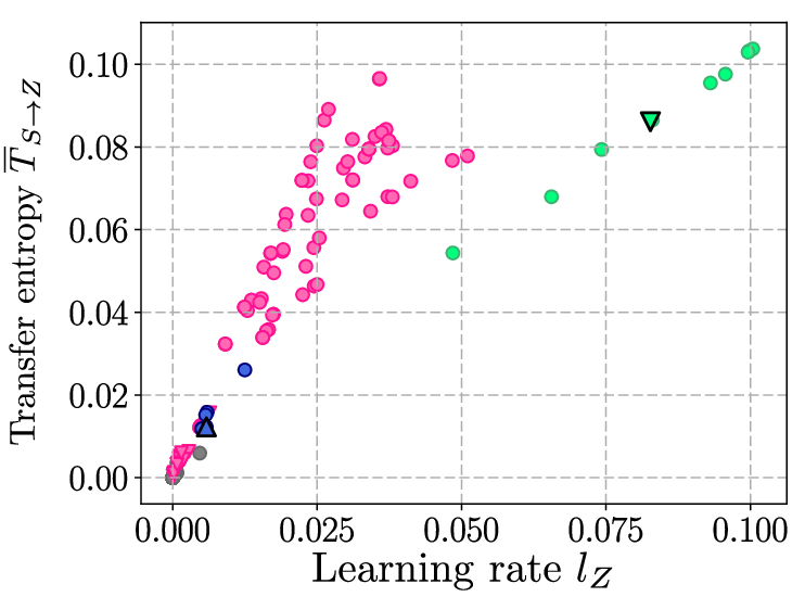
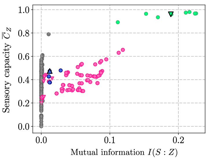
In the setup of Fig. 2, we classify all the three-node patterns on the basis of information-thermodynamic quantities. We reveal that patterns are classified into four types and to which type each network motif belongs. We show scatter plots with respect to several information-thermodynamic quantities in Fig. 3. Fig. 3 and Fig. 3 show information-thermodynamic dissipation $D_{Z}$ and $D_{\rm all}$ . Figure 3 and Fig. 3 show four information quantities. All the points split into four groups in Fig. 3 and 3. We also realize that the group with the second smallest dissipation split into two groups in Fig. 3 and 3. From these observations, we assign different colors and shapes to the patterns in Fig. 3. These five groups can be rearranged into four types on the basis of their characteristics as shown in Table. 1. Here, the sensory capacity plays a role in the separation of the groups. For example, the mutual information of M11-1-4 (which belongs to and $I(S:Z)\sim 0.1$ ) is small, but its sensory capacity is big. We discuss the characteristic of each type below. Also, the concrete behavior of the patterns in each type is shown by simulation in Appendix D. First, and are dissipative groups. We confirmed that all the patterns in and include negative feedback loops. The reason why they are dissipative is that they show oscillatory behavior due to such negative feedback loops. On the other hand, the patterns in dissipate much less. These patterns also take small values in terms of the information quantities. We confirmed that all of them include positive feedback loops. The behavior of these patterns is due to the fact that dynamics of these patterns are static because of positive feedback loops, and they do not react well to the signals from $S$ . The remaining 17 patterns that belong to and are shown in Fig. 4. The patterns in take small values in terms of the information quantities, and the other way around for the patterns in . We find that the patterns in include incoherent feedforward loops. According to the simulation results shown in Appendix D, they show adaptive behavior such that they pass information from $S$ to $Z$ only in a short time when the state of $S$ changes. For example, in the case of M5-1-2 (I1), $Z$ changes from 0 to 1 temporarily when $X$ changes from 0 to 1, but after that, $Z$ returns to 0 due to the inhibition by $Y$ . This is the reason why the patterns in take small values in terms of the information quantities. We finally confirm that the patterns in propagate signals from $S$ to $Z$ quite well. Thus, these patterns take large values in terms of the information quantities. The CFFL and IFFL network motifs are classified into and respectively, and the PFBL network motifs belong to the or type (see Appendix D.4 for the details of the classification of the PFBL network motifs). Interestingly, there are only two types other than , and , and the CFFLs and IFFLs are simple patterns in and . No network motifs belong to the dissipative type . In terms of information thermodynamics, the dissipative type might waste too much chemical fuels, which may be one of the reasons why no network motifs belong to the dissipative type. The and types are interesting because they operate with small dissipation and have the capability of propagating information. The patterns in form a stable correlation, and those in propagate information temporarily. The patterns that propagate information would be preferable in gene regulatory networks because the upstream gene can control the state of the pattern. We will discuss the reason why feedforward loops are distinguished from the other patterns in and in the next subsection.

III.2 Two inputs: Logical operation

We now show our second result. Besides the input to $X$ , in real gene regulatory networks, a three-node pattern often takes another input to $Y$ . Therefore, patterns that can nontrivially operate on both the signals would be preferable in natural selection. Here we evaluate the capacity of logical operation performed by three-node patterns by using an information quantity called tripartite mutual information, and discuss the reason why patterns with fewer edges such as feedforward loops are preferred. We consider the situation that two signal sources $S_{1}$ and $S_{2}$ activate $X$ and $Y$ independently (Fig. 5), and that $S_{1}$ and $S_{2}$ flip between 0 and 1 randomly (i.e., $e_{S_{1}}=e_{S_{2}}=1$ ). The parameters are set with the following conditions:

	$\displaystyle\gamma_{S}:=\gamma_{S_{1}}=\gamma_{S_{2}},$		(21)
	$\displaystyle\gamma:=\gamma_{X}=\gamma_{Y}=\gamma_{Z},$		(22)
	$\displaystyle\gamma_{S}\ll\gamma,$		(23)
	$\displaystyle e:=e_{X}=e_{Y}=e_{Z}\ll 1.$		(24)

We exclude irrelevant patterns from calculation with the same rule as in Sec. III.1, and additionally exclude patterns that become equivalent by swapping $X$ and $Y$ . As a result, we perform calculation for 204 patterns (see Appendix C for the details). We discuss the definition and the basic properties of tripartite mutual information [59], which quantifies how nontrivially the output $Z$ depends on the inputs $S_{1}$ and $S_{2}$ . The tripartite mutual information between these three nodes is defined as

$\displaystyle I_{3}(S_{1},S_{2},Z)$	$\displaystyle:=$	$\displaystyle H(S_{1})+H(S_{2})+H(Z)-H(S_{1},S_{2})$
		$\displaystyle-H(S_{1},Z)-H(S_{2},Z)+H(S_{1},S_{2},Z)$
	$\displaystyle=$	$\displaystyle I(S_{1}:Z)+I(S_{2}:Z)-I(\{S_{1},S_{2}\}:Z).$

To illustrate the informational meaning of tripartite mutual information, we show two examples with three binary bits $x,y,z$ : (i) $I_{3}(x,y,z)=-\ln 2$ if $x=y\oplus z$ (XOR), and $y$ and $z$ are independent and random. In this case, neither $y$ nor $z$ is correlated with $x$ , while composite $yz$ has maximum correlation with $x$ . This means that information of $y$ and that of $z$ are mixed up in $x$ . (ii) $I_{3}(x,y,z)=\ln 2$ if $x=y=z$ and $x$ is random. In this case, three bits are maximally correlated. These examples show that the negative tripartite mutual information quantifies mixing of signals from two inputs ( $y$ and $z$ in this case). In the present setup, it does not take a positive value, as shown from simple calculation with the assumption $I(S_{1}:S_{2})=H(S_{1})+H(S_{2})-H(S_{1},S_{2})=0$ . In fact, we have

$\displaystyle I_{3}(S_{1},S_{2},Z)$	$\displaystyle=$	$\displaystyle H(Z)+H(S_{2})-H(S_{2},Z)-H(S_{2})$	(26)
		$\displaystyle-H(S_{1},Z)+H(S_{1},S_{2},Z)$
	$\displaystyle=$	$\displaystyle I(S_{2}:Z)-I(S_{2}:\{S_{1},Z\})$
	$\displaystyle\leq$	$\displaystyle 0.$

The smaller the tripartite mutual information is, the more non-trivial the logical operation is. In fact, if $Z$ depends on both $S_{1}$ and $S_{2}$ , $I(S_{1}:Z)+I(S_{2}:Z)$ becomes smaller than $I(\{S_{1},S_{2}\}:Z)$ , which implies a small negative value of $I_{3}(S_{1},S_{2},Z)$ (or equivalently, the absolute value $|I_{3}(S_{1},S_{2},Z)|$ becomes large). The logical operation is non-trivial in this case. On the other hand, if $Z$ depends only on $S_{1}$ and is independent of $S_{2}$ , $I(S_{1}:Z)=I(\{S_{1},S_{2}\}:Z)$ and $I(S_{2}:Z)=0$ hold, resulting in $I_{3}(S_{1},S_{2},Z)=0$ , where the logical operation is trivial. We argue that a pattern with small tripartite mutual information is preferable in gene regulatory networks because of the following reason. If the tripartite mutual information is small, both information from $S_{1}$ and $S_{2}$ propagate to $Z$ , which enables the pattern to process information in a complex way. In fact, a previous study shows that information propagates more widely in gene regulatory networks than in random networks [60]. We show the result of our calculation in Fig. 6. The horizontal axis is the mutual information $I(\{S_{1},S_{2}\}:Z)$ , and the vertical axis is the tripartite mutual information $I_{3}(S_{1},S_{2},Z)$ . Network motifs M5-1-1 and M5-1-2 take small values of the tripartite mutual information. There are only six patterns that take small values of the tripartite mutual information, which are shown with a brace in Fig. 6. These six patterns are listed in Fig. 7. Interestingly, these six patterns have only a few edges, which may explain the reason why gene regulatory networks consist of patterns with fewer edges.

There seems to be a bifurcation structure in Fig. 6. The upper left patterns do not propagate information at all, i.e., $I(\{S_{1},S_{2}\}:Z)\simeq 0$ , and the upper right patterns make $Z$ only react to one of the two signals $S_{1}$ or $S_{2}$ . On the basis of these observations, we consider two simple models (Fig. 6(b)(c)) that explain the bifurcation structure. Intuitively speaking, these two models capture the following properties: (i) how much information propagates from $S_{1}$ or $S_{2}$ to $Z$ , and (ii) how equally information propagates in the two paths. In the model of Fig. 6, the NOT gates are inserted into the two inputs with probability $\varepsilon$ independently. In this model, the NOT gates represent the errors that independently occur on the input signals during the logical operation. In the model of Fig. 6, the probability of inserting the NOT gates is fixed with $\varepsilon_{0}$ , and one of the AND gate or a straight pass from $S_{1}$ to $Z$ is chosen with probabilities $\varepsilon$ and $1-\varepsilon$ , respectively. In this model, the non-triviality of the logical operation is represented by the probability $\varepsilon$ . The left curve in Fig. 6 is drawn with model 6 by varying $\varepsilon$ in the range of $\varepsilon_{0}\leq\varepsilon\leq 0.5$ , and the right curve is drawn with model 6 by varying $\varepsilon$ in $0\leq\varepsilon\leq 1$ . Here, there is only a single fitting parameter $\varepsilon_{0}$ . The good agreement with the data means that these models capture the essence of the behavior of the three-node patterns. In particular, network motifs M5-1-1 and M5-1-2 perform non-trivial logical operation with relatively small errors. On the other hand, most of the patterns in perform trivial logical operation, and the patterns in other than M5-1-2 do not propagate information at all. We can thus consider that these patterns are unfavorable in terms of information processing. We note that M4-1-1 is not a network motif. It should be remarked, however, that M4-1-1 occurs most frequently in many gene regulatory networks [14], and it also occurs frequently in random networks (and thus is not regarded as a network motif). In this way, tripartite mutual information gives us an intuitive account for not only network motifs but also frequent patterns in gene regulatory networks. The above result may give a reasonable explanation for the difference in the occurrence frequencies among different types of feedforward loops. As shown in Fig. 1, there are eight types of feedforward loops, but only the C1 and I1 FFLs occur most frequently with around 40 percent and 30 percent each, and the other six types occur with around five percent each. This has been confirmed in the gene regulatory networks of E. coli and S. cerevisiae [8]. The tripartite mutual information of C3, C4, I3 and I4 is around zero in Fig. 6. Since a pattern whose tripartite mutual information is around 0 is trivial in terms of logical operation, this may explain the low occurrence frequencies of C3, C4, I3 and I4 FFLs, which suggests that the value of tripartite mutual information indeed quantifies the capability of logical operation of three-node patterns. It should be noted that we assumed each regulatory function as the AND gate in the foregoing argument. If the regulatory function of a three-node pattern is given by a combination of AND and OR, the conclusion becomes opposite to the above (see Appendix B for the details). Therefore, it is a future issue to check the consistency between our result and real experimental data. Qualitatively the same argument has also been mentioned in Refs. [6, 7]. In Refs. [6, 7], the authors argued that the eight types of FFLs are different with each other, in that stationary $Z$ shows different dependence on the two signal molecules (which correspond to $S_{1}$ and $S_{2}$ in this study). In the present work, we clarify the different dependence by using tripartite mutual information.

IV Concluding remarks

In a system like a gene regulatory network with information propagation, it is crucial to take into account information flow to analyze dissipation. In this study, we have adopted information thermodynamics to quantify such dissipation in a three-node pattern which is only a part of a large-scale network. We first considered the case where there is a single input, and characterized all the possible three-node patterns with information-thermodynamic quantities. We found that these patterns are classified into four types. We discussed the characteristics of network motifs, by considering to which types they are categorized. We next considered the case where there are two inputs. By quantifying how the two inputs affect the output by tripartite mutual information, we argued the reason why feedforward-loop network motifs occur frequently in an intuitive manner. This result is consistent with a previous study which claims that information propagates more widely in gene regulatory networks than in random networks [60]. In addition, we found that the different occurrence frequencies among the eight types of feedforward loops might correspond to the difference in the amounts of tripartite mutual information. We have partly succeeded to explain in what respect network motifs have advantages compared to other patterns in terms of information-thermodynamic quantities. We note that previous studies [7, 5] explain that IFFL network motifs would be preferable because they show adaptive behavior and accelerate the response time. On the other hand, we argue that IFFLs are preferable because they show adaptive behavior with small dissipation and they take small tripartite mutual information. We believe that these two approaches are complimentary to each other. However, these results might involve some uncertainty due to the fact that the stochastic Boolean model might be too much simplified. Although this model is suitable for understanding the basic behavior of gene regulatory patterns, the oscillatory or static solution often deviates from the actual behavior. In addition, since the stochastic Boolean model is a coarse-grained model, some dissipative processes such as protein productions are not included. Therefore, it is a future issue to investigate dissipation by using more detailed models. For example, the difference in the occurrence frequencies between C1 (I1) and C2 (I2) might be accounted for by such detailed analysis of dissipation. Meanwhile, our study suggests that tripartite mutual information is important in terms of the network formation of gene regulatory networks. The symmetry between the occurrence frequencies of the C1 to C4 and the I1 to I4 FFLs [8] may arise from the symmetry in the tripartite mutual information between them. It is also worth investigating whether the same tendencies can be found in other gene regulatory networks than those of E.coli and S.cerevisiae. Our results suggest that information thermodynamics gives us a useful methodology for a systematic analysis of biochemical reaction networks. We note that tripartite mutual information has not received much attention in this context so far, while information quantities such as mutual information and transfer entropy have often been used in a wide context[61, 62]. Further application of our approach to a broader class of networks, including both biological and artificial ones, is a future issue.

Acknowledgements.

We thank Tetsuya J. Kobayashi for fruitful discussion. T. S. is supported by JSPS KAKENHI Grant No. JP16H02211 and No. 25103003.

Appendix A Master equation

In this appendix, we present an example of the master equation for the stochastic Boolean model. We consider the pattern described in Fig. 2 as an example. The joint probability distribution $p(s_{t},x_{t},y_{t},z_{t})$ is represented by the probability vector $\bm{p}$ defined by

	$\displaystyle\bm{p}=(p(0,0,0,0),p(0,0,0,1),p(0,0,1,0),p(0,0,1,1),$
	$\displaystyle p(0,1,0,0),p(0,1,0,1),p(0,1,1,0),p(0,1,1,1),$
	$\displaystyle p(1,0,0,0),p(1,0,0,1),p(1,0,1,0),p(1,0,1,1),$
	$\displaystyle p(1,1,0,0),p(1,1,0,1),p(1,1,1,0),p(1,1,1,1))^{\mathrm{T}},$		(29)

where T means the transpose of a matrix. Then the transition matrix $H$ is given by

\displaystyle H=\left(\begin{matrix}A&B\\ C&D\\ \end{matrix}\right),

(30)

where

	$\displaystyle A=$
	$\displaystyle\left(\begin{matrix}&\gamma_{Z}&e_{Y}\gamma_{Y}&0&\gamma_{X}&0&0&0\\ e_{Z}\gamma_{Z}&&0&e_{Y}\gamma_{Y}&0&\gamma_{X}&0&0\\ \gamma_{Y}&0&&\gamma_{Z}&0&0&\gamma_{X}&0\\ 0&\gamma_{Y}&e_{Z}\gamma_{Z}&&0&0&0&\gamma_{X}\\ e_{X}\gamma_{X}&0&0&0&&\gamma_{Z}&\gamma_{Y}&0\\ 0&e_{X}\gamma_{X}&0&0&e_{Z}\gamma_{Z}&&0&\gamma_{Y}\\ 0&0&e_{X}\gamma_{X}&0&e_{Y}\gamma_{Y}&0&&e_{Z}\gamma_{Z}\\ 0&0&0&e_{X}\gamma_{X}&0&e_{Y}\gamma_{Y}&\gamma_{Z}&\\ \end{matrix}\right),$

	$\displaystyle D=$
	$\displaystyle\left(\begin{matrix}&\gamma_{Z}&e_{Y}\gamma_{Y}&0&e_{X}\gamma_{X}&0&0&0\\ e_{Z}\gamma_{Z}&&0&e_{Y}\gamma_{Y}&0&e_{X}\gamma_{X}&0&0\\ \gamma_{Y}&0&&\gamma_{Z}&0&0&e_{X}\gamma_{X}&0\\ 0&\gamma_{Y}&e_{Z}\gamma_{Z}&&0&0&0&e_{X}\gamma_{X}\\ \gamma_{X}&0&0&0&&\gamma_{Z}&\gamma_{Y}&0\\ 0&\gamma_{X}&0&0&e_{Z}\gamma_{Z}&&0&\gamma_{Y}\\ 0&0&\gamma_{X}&0&e_{Y}\gamma_{Y}&0&&e_{Z}\gamma_{Z}\\ 0&0&0&\gamma_{X}&0&e_{Y}\gamma_{Y}&\gamma_{Z}&\\ \end{matrix}\right),$

and $B=C=\gamma_{S}I$ with $I$ being the identity matrix. Here, an element represented by $*$ above is determined so that the sum of each column becomes zero. For example, the $(1,1)$ element of $H$ is given by $H_{11}=-e_{X}\gamma_{X}-\gamma_{Y}-e_{Z}\gamma_{Z}-\gamma_{S}$ . The time evolution of the total system is described by the master equation

\displaystyle\frac{d\bm{p}}{dt}=H\bm{p}.

(33)

For example, the first row of the above equation is given by

$\displaystyle\frac{dp(0,0,0,0)}{dt}$	$\displaystyle=$	$\displaystyle H_{11}p(0,0,0,0)+\gamma_{Z}p(0,0,0,1)$	(34)
	$\displaystyle+$	$\displaystyle e_{Y}\gamma_{Y}p(0,0,1,0)+\gamma_{X}p(0,1,0,0)$
	$\displaystyle+$	$\displaystyle\gamma_{S}p(1,0,0,0).$

Appendix B Equivalence of network patterns

In this appendix, we first formulate the equivalence of network patterns and then discuss the relation between the OR-logic patterns and the AND-logic ones.

B.1 Definition of the equivalence

We consider the stationary state of the setup in Fig. 2. We show the definition of the equivalence of two patterns by an example. If the join probability distributions $p_{1}(s_{t},x_{t},y_{t},z_{t},s_{t+dt},x_{t+dt},y_{t+dt},z_{t+dt})$ for a pattern 1 and $p_{2}(s_{t},x_{t},y_{t},z_{t},s_{t+dt},x_{t+dt},y_{t+dt},z_{t+dt})$ for another pattern 2 satisfy the following relation for all $s_{t},x_{t},y_{t},z_{t},s_{t+dt},x_{t+dt},y_{t+dt},z_{t+dt}\in\{0,1\}$ , then patterns 1 and 2 are said to be equivalent:

	$\displaystyle p_{1}(s_{t},x_{t},y_{t},z_{t},s_{t+dt},x_{t+dt},y_{t+dt},z_{t+dt})=$
	$\displaystyle p_{2}(s_{t},x_{t},y_{t},\overline{z_{t}},s_{t+dt},x_{t+dt},y_{t+dt},\overline{z_{t+dt}}),$		(35)

where the bar on a letter represents the inversion $0\mapsto 1$ and $1\mapsto 0$ . In general, the inversion is allowed on multiple nodes, but it should be performed on both variables at time $t$ and at time $t+dt$ simultaneously. If pattern 1 and 2 are equivalent, their information quantities take the same values. For example, when Eq. (35) holds, the mutual information $I_{1}(S_{t},Z_{t})$ for pattern 1 and $I_{2}(S_{t},Z_{t})$ for pattern 2 become the same:

$\displaystyle I_{1}(S_{t}:Z_{t})$	$\displaystyle=$	$\displaystyle\sum_{s_{t},z_{t}}p_{1}(s_{t},z_{t})\ln\frac{p_{1}(s_{t},z_{t})}{p_{1}(s_{t})p_{1}(z_{t})}$	(36)
	$\displaystyle=$	$\displaystyle\sum_{s_{t},z_{t}}p_{2}(s_{t},\overline{z_{t}})\ln\frac{p_{2}(s_{t},\overline{z_{t}})}{p_{2}(s_{t})p_{2}(\overline{z_{t}})}$
	$\displaystyle=$	$\displaystyle\sum_{s_{t},z_{t}}p_{2}(s_{t},z_{t})\ln\frac{p_{2}(s_{t},z_{t})}{p_{2}(s_{t})p_{2}(z_{t})}$
	$\displaystyle=$	$\displaystyle I_{2}(S_{t}:Z_{t}).$

This equivalence of patterns can be shown graphically. For example, Fig. 8 shows a transformation from one pattern to another equivalent pattern.

This transformation is based on the following equations: $f^{\overline{X}}={\rm NOT}(S_{t})$ (if $f^{X}=S_{t}$ for example), and $f^{i}(X,...)=f^{i}(\overline{\overline{X}},...)~(i=Y~{\rm or}~Z)$ . We discuss the equivalence among feedforward loops. In the setup of Fig. 2, the equivalent transformation on $X$ and $Y$ is possible. Thus, the patterns from the C1 to C4 and those from the I1 to I4 FFLs become equivalent, respectively. On the other hand, in the setup of Fig. 5, the transformation is possible only on $X$ , because if we make the transformation on $Y$ , the regulatory function of $Y$ changes accordingly (see Fig. 9). In this case, the C1 and C2, the C3 and C4, the I1 and I2, the I3 and I4 FFLs become equivalent, respectively.

B.2 Equivalence between the OR-logic patterns and the AND-logic ones

In this study, we have assumed that the regulatory functions are given by the AND gates, but there is other type of gene whose regulatory function can be described by the OR gate. Even if we assume the regulatory functions of a pattern to be a combination of the AND and OR gates, the scatter plots of Fig. 3 and Fig. 6 themselves do not change, while a pattern that corresponds to each point becomes different from that of Fig. 3 and Fig. 6. Therefore, it is enough to consider the mapping from a pattern with the AND and OR gates to a pattern with only the AND gates on the basis of the equivalent transformation. We first consider the results in Fig. 3 that are independent of the regulatory functions. (i) The points of the FFLs are independent of the choice of the regulatory functions in Fig. 3 (see Fig. 10). Therefore, the CFFLs belong to the informative type and the IFFLs belong to the adaptive type independently of the regulatory functions. (ii) No network motifs belong to the dissipative type. This is because a negative feedback loop is mapped to a negative feedback loop by the equivalent transformation, and it is still a necessary condition to belong to the dissipative type that a pattern includes negative feedback loops. We next consider the results in Fig. 3 that are dependent on the regulatory functions. The classification of the positive feedback loop network motifs are dependent on the choice of regulatory functions. This is because a positive feedback loop shows two distinct behavior “static” or “bistable” depending on the regulatory functions (see Appendix D.4 and Fig. 19). We also consider the results in Fig. 6 that are dependent on the regulatory functions. The tripartite mutual information of the FFLs are dependent on the regulatory functions. In the setup of Fig. 5, for example, let us consider a situation that the regulatory functions of Y and Z nodes of the C1 FFL are AND and OR respectively. If we express this as C1(AND, OR), C1(AND, OR) is equivalent to C3(AND, AND) as shown in Fig. 11. By considering the other cases in the same manner, we can summarize the dependence of the results on the regulatory functions as Table 2. It mat be possible to explain the difference in the occurrence frequencies among the FFLs by the statistical tendency in the regulatory functions. This is because the FFLs which have similar occurrence frequencies are categorized into the same subgroups C1, I1, C2, I2 and C3, I3, C4, I4. If the combination of (AND, AND) or (OR, OR) occurs more frequently than (AND, OR) or (OR, AND), for example, we can expect that the C1, I1, C2, I2 FFLs occur more frequently than the C3, I3, C4, I4 FFLs. It is a remaining question why the occurrence frequencies of the C2 and I2 FFLs are low comparing to the C1 and I1 FFLs.

	C1, I1, C2, I2	C3, I3, C4, I4
(AND, AND), (OR, OR)	small	around 0
(AND, OR), (OR, AND)	around 0	small

Table 2: The tripartite mutual information of the FFLs are dependent on the regulatory functions. The vertical column represents the regulatory functions of (Y, Z) and the horizontal column represents the two types of the FFLs.

Appendix C Irrelevant patterns

There are totally $3^{6}-8\cdot 3-1=704$ three-node patterns, but some of them are irrelevant. In this study we exclude patterns from calculation with the following rules: (i) patterns without causal relationship from $X$ to $Z$ or $Y$ to $Z$ , (ii) patterns that have unregulated nodes. Two examples of the case (i) are shown in Fig. 12, where $Y$ does not regulate $X$ or $Z$ in these patterns. Since such patterns are equivalent to some two-node patterns, we exclude them from our calculation.

Two examples of the case (ii) are shown in Fig. 13. Patterns without regulation of $Y$ are equivalent to some two-node patterns in the setup of Fig. 2, while patterns without regulation of $Z$ are meaningless.

Moreover, in the setup of Fig. 5, the roles of $X$ and $Y$ become equivalent. We calculated only one of patterns that become equivalent by swapping nodes $X$ and $Y$ (Fig. 14).

In summary, we include only a single pattern out of equivalent ones for our calculation on the basis of the above rules. As a result, we performed our calculation for 283 patterns for the setup of Fig. 2 and 204 patterns for the setup of Fig. 5 (see Supplemental Material for the list of these patterns).

Appendix D Dynamics of patterns

In this Appendix, we show the characteristics of the four types shown in Table. 1 with examples of numerical simulation based on the Gillespie method [63]. In addition, we argue the function of a positive feedback loop by using two examples. From Fig. 15 to Fig. 17, we show the time evolution of $X$ , $Y$ and $Z$ when $S$ changes with a constant period. For simplicity, we set $e=0$ , while $\gamma=1$ as in Fig. 3.

D.1 Pink type: Dissipative

M9-1-2 belongs to , and M10-3-4 belongs to , which are respectively shown in Fig. 15(a) and 15(b). Both of them include negative feedback loops, and are dissipative types. We can see oscillatory behavior. In M10-3-4, $Z$ shows oscillations independently of $S_{t}$ , while in M9-1-2, $Z$ shows oscillations only when $S_{t}$ is 1. Thus we argue that this difference leads to the difference in the dissipation of and .

D.2 Gray type: Static

M11-1-1 belongs to , which includes a positive feedback loop. We can see that $Z$ converges to a stationary value.

D.3 Green and blue types: Informative and adaptive

M11-1-8 belongs to the informative type and M10-5-6 belongs to the adaptive type , which are shown in Fig. 17(a) and 17(b), respectively. In M11-1-8, the variation in $S$ propagates to $Z$ as it is, while in M10-5-6, $Z$ reacts only when $S$ changes from 0 to 1.

D.4 Positive feedback loop: Static or Bistable

A positive feedback loop has two functions depending on the signs of the two regulations. A positive feedback loop composed of two positive regulations has a static property, and that composed of two negative regulations is bistable (see Fig. 16(a), 17(a) and 18). Here, we assume that the regulatory functions are the AND gates. Thus, although most of the PFBL network motifs belong to the gray type, some of them are classified into the green type (Fig. 19). Therefore, it is necessary to check the signs and the logics of the regulatory functions when we discuss the role of the PFBL network motifs in gene regulatory networks.

Appendix E Details of the fitting in Fig. 6

We show the details of the fitting curves in Fig. 6. For example, the probability distribution of the model of Fig. 6 is given by

$\displaystyle P(S_{1}=0,S_{2}=0,Z=0)$	$\displaystyle=$	$\displaystyle\frac{1}{4}\left\{\varepsilon\cdot(1-\varepsilon_{0}\cdot\varepsilon_{0})\right.$	(40)
		$\displaystyle\left.+(1-\varepsilon)\cdot(1-\varepsilon_{0})\right\},$	(40)
$\displaystyle P(S_{1}=0,S_{2}=0,Z=1)$	$\displaystyle=$	$\displaystyle\frac{1}{4}\left\{\varepsilon\cdot\varepsilon_{0}\cdot\varepsilon_{0}\right.$	(41)
		$\displaystyle\left.+(1-\varepsilon)\cdot\varepsilon_{0}\right\},$	(41)
$\displaystyle P(S_{1}=1,S_{2}=0,Z=0)$	$\displaystyle=$	$\displaystyle\frac{1}{4}\left\{\varepsilon\cdot(1-(1-\varepsilon_{0})\cdot\varepsilon_{0})\right.$	(42)
		$\displaystyle\left.+(1-\varepsilon)\cdot\varepsilon_{0}\right\},$	(42)
$\displaystyle P(S_{1}=1,S_{2}=0,Z=1)$	$\displaystyle=$	$\displaystyle\frac{1}{4}\left\{\varepsilon\cdot(1-\varepsilon_{0})\cdot\varepsilon_{0}\right.$	(43)
		$\displaystyle\left.+(1-\varepsilon)\cdot(1-\varepsilon_{0})\right\},$	(43)
$\displaystyle P(S_{1}=0,S_{2}=1,Z=0)$	$\displaystyle=$	$\displaystyle\frac{1}{4}\left\{\varepsilon\cdot(1-(1-\varepsilon_{0})\cdot\varepsilon_{0})\right.$	(44)
		$\displaystyle\left.+(1-\varepsilon)\cdot(1-\varepsilon_{0})\right\},$	(44)
$\displaystyle P(S_{1}=0,S_{2}=1,Z=1)$	$\displaystyle=$	$\displaystyle\frac{1}{4}\left\{\varepsilon\cdot(1-\varepsilon_{0})\cdot\varepsilon_{0}\right.$	(45)
		$\displaystyle\left.+(1-\varepsilon)\cdot\varepsilon_{0}\right\},$	(45)

$\displaystyle P(S_{1}=1,S_{2}=1,Z=0)$	$\displaystyle=$	$\displaystyle\frac{1}{4}\left\{\varepsilon\cdot(1-(1-\varepsilon_{0})\cdot(1-\varepsilon_{0}))\right.$	(46)
		$\displaystyle\left.+(1-\varepsilon)\cdot\varepsilon_{0}\right\},$	(46)
$\displaystyle P(S_{1}=1,S_{2}=1,Z=1)$	$\displaystyle=$	$\displaystyle\frac{1}{4}\left\{\varepsilon\cdot(1-\varepsilon_{0})\cdot(1-\varepsilon_{0})\right.$	(47)
		$\displaystyle\left.+(1-\varepsilon)\cdot(1-\varepsilon_{0})\right\}.$	(47)

Then, $I(\{S_{1},S_{2}\}:Z)$ and $I_{3}(S_{1},S_{2},Z)$ are determined as functions of $\varepsilon_{0}$ and $\varepsilon$ by putting the above expressions into their definitions.

Appendix F Parameter dependence of the main results

We discuss the parameter dependence of Fig. 3 and Fig. 6. For example, Fig. 20(a) represents the case where $\gamma_{S}$ is set to 0.01, while the other parameters are kept in the same values as those of Fig. 3. We note that the information-thermodynamic dissipation diverges and thus is meaningless for $e=0$ . We show the cases of various parameters in Fig. 20 to Fig. 22. There are some cases where the type classification become ambiguous, but it can be reasonably understood by considering the characteristics of individual types, as discussed below. The classification becomes the most ambiguous in the case of $\gamma_{S}=1$ . This is the case where the signal changes before the system relaxes, which is unrealistic in real biological systems. The case where the classification becomes ambiguous the second most is $e=0.1$ . This is the case where stochasticity of the system is too large, and the static nature of positive feedback loops disappears, leading to the small difference between and . In Fig. 23, we show scatter plots of the tripartite mutual information. The models of Fig. 6 and 6 do not fit well with the data in Fig. 23(b), 23(c), 23(d), and 23(f). However, the conclusion does not change from that of Fig. 6. For example, M4-1-1, M5-1-1 and M5-1-2 still take smaller values in terms of the tripartite mutual information in the plots of Fig. 23. The reason why the models in Fig. 6 do not fit well with the data in Fig. 23(c) and 23(d) is that these models suppose the symmetric properties between $X$ and $Y$ . On the other hand, in Fig. 23 23(a) and 23(e), the models fit well with the data, and the fitting parameters are determined as (a) $\varepsilon_{0}=0.022$ , (e) $\varepsilon_{0}=0.153$ .

References

[1] Y. Taniguchi, P. J. Choi, G. W. Li, H. Chen, M. Babu, J. Hearn, A. Emili and X. S. Xie, Quantifying E. coli Proteome and Transcriptome with Single-Molecule Sensitivity in Single Cells, Science 329, 533 (2010).
[2] S. S. Shen-Orr, R. Milo, S. Mangan, and U. Alon, Network motifs in the transcriptional regulation network of Escherichia coli, Nat. Genet. 31, 64 (2002).
[3] R. Milo, S. Shen-Orr, S. Itzkovitz, N. Kashtan, D. Chklovskii and U. Alon, Network Motifs: Simple Building Blocks of Complex Networks, Science 298, 824 (2002).
[4] T. I. Lee, N. J. Rinaldi, F. Robert, D. T. Odom, Z. Bar-Joseph, G. K. Gerber, N. M. Thompson, I. Simon, J. Zeitlinger, E. G. Jennings, H. L. Murray, D. B. Gordon, B. Ren, J. J. Wyrick, J.-B. Tagne, T. L. Volkert, E. Fraenkel, D. K. Gifford and R. A. Young, Transcriptional Regulatory Networks in Saccharomyces cerevisiae, Science 298, 799 (2002).
[5] U. Alon, Network motifs: theory and experimental approaches, Nat. Rev. Genet. 8, 450 (2007).
[6] S. Mangan and U. Alon, Structure and function of the feed-forward loop network motif, P. Natl. Acad. Sci. USA 100, 11980 (2003).
[7] U. Alon, An Introduction to Systems Biology, (CRC Press, 2006).
[8] S. Mangan, S. Itzkovitz, A. Zaslaver, and U. Alon, The incoherent feed-forward loop accelerates the response-time of the gal system of Escherichia coli, J. Mol. Biol. 356, 1073 (2006).
[9] M. Kittisopikul and G. M. Suel, Biological role of noise encoded in a genetic network motif, P. Natl. Acad. Sci. USA 107, 13300 (2010).
[10] L. T. MacNeil and A. J. M. Walhout, Gene regulatory networks and the role of robustness and stochasticity in the control of gene expression, Genome Res. 21, 645 (2011).
[11] W. H. De Ronde, F. Tostevin, and P. R. Ten Wolde, Feed-forward loops and diamond motifs lead to tunable transmission of information in the frequency domain, Phys. Rev. E 86 (2012).
[12] L. Albergante, J. J. Blow, and T. J. Newman, Buffered Qualitative Stability explains the robustness and evolvability of transcriptional networks, eLife 3, e02863 (2014).
[13] G. Swiers, R. Patient, and M. Loose, Genetic regulatory networks programming hematopoietic stem cells and erythroid lineage specification, Dev. Biol. 294, 525 (2006).
[14] M. B. Gerstein, A. Kundaje, M. Hariharan, S. G. Landt, K. K. Yan, C. Cheng, X. J. Mu, E. Khurana, J. Rozowsky, R. Alexander, R. Min, P. Alves, A. Abyzov, N. Addleman, N. Bhardwaj, A. P. Boyle, P. Cayting, A. Charos, D. Z. Chen, Y. Cheng, D. Clarke, C. Eastman, G. Euskirchen, S. Frietze, Y. Fu, J. Gertz, F. Grubert, A. Harmanci, P. Jain, M. Kasowski, P. Lacroute, J. Leng, J. Lian, H. Monahan, H. Ogeen, Z. Ouyang, E. C. Partridge, D. Patacsil, F. Pauli, D. Raha, L. Ramirez, T. E. Reddy, B. Reed, M. Shi, T. Slifer, J. Wang, L. Wu, X. Yang, K. Y. Yip, G. Z.-Schapira, S. Batzoglou, A. Sidow, P. J. Farnham, R. M. Myers, S. M. Weissman and M. Snyder, Architecture of the human regulatory network derived from ENCODE data, Nature 489, 91 (2012).
[15] R. Prill, P. Iglesias, A. Levchenko, Dynamic properties of network motifs contribute to biological network organization, PloS Biol. 3 (11): e343. (2005).
[16] C. Jarzynski, Hamiltonian Derivation of a Detailed Fluctuation Theorem, J. Stat. Phys. 98, 77 (2000).
[17] K. Sekimoto, Stochastic Energetics (Springer, 2010).
[18] U. Seifert, Stochastic thermodynamics, fluctuation theorems and molecular machines, Rep. Prog. Phys. 75, 126001 (2012).
[19] T. Sagawa and M. Ueda, Generalized Jarzynski equality under nonequilibrium feedback control, Phys. Rev. Lett. 104, 1 (2010).
[20] S. Toyabe, T. Sagawa, M. Ueda, E. Muneyuki, and M. Sano, Experimental demonstration of information-to-energy conversion and validation of the generalized Jarzynski equality, Nat. Phys. 6, 988 (2010).
[21] T. Sagawa and M. Ueda, Fluctuation Theorem with Information Exchange: Role of Correlations in Stochastic Thermodynamics, Phys. Rev. Lett. 109, 180602 (2012).
[22] S. Ito and T. Sagawa, Information thermodynamics on causal networks, Phys. Rev. Lett. 111, 1 (2013).
[23] J. M. Horowitz and M. Esposito, Thermodynamics with Continuous Information Flow, Phys. Rev. X 4, 031015 (2014).
[24] J. M. Horowitz and H. Sandberg, Second-law-like inequalities with information and their interpretations, New J. Phys. 16, 125007 (2014).
[25] J. M. R. Parrondo, J. M. Horowitz, and T. Sagawa, Thermodynamics of information, Nat. Phys. 11, 131 (2015).
[26] N. Shiraishi and T. Sagawa, Fluctuation theorem for partially masked nonequilibrium dynamics, Phys. Rev. E 91, 3 (2015).
[27] P. Sartori, L. Granger, C. F. Lee, and J. M. Horowitz, Thermodynamic Costs of Information Processing in Sensory Adaptation, PLoS Comput. Biol. 10, e1003974 (2014).
[28] A. C. Barato, D. Hartich, and U. Seifert, Efficiency of cellular information processing, New J. Phys. 16, 103024 (2014).
[29] S. Ito and T. Sagawa, Maxwell’s demon in biochemical signal transduction with feedback loop, Nat. Commun. 6, 7498 (2015).
[30] D. Hartich, A. C. Barato, and U. Seifert, Sensory capacity: An information theoretical measure of the performance of a sensor, Phys. Rev. E 93, 1 (2016).
[31] T. E. Ouldridge, C. C. Govern, and P. R. ten Wolde, Thermodynamics of Computational Copying in Biochemical Systems, Phys. Rev. X 7, 021004 (2017).
[32] T. Matsumoto and T. Sagawa, Role of sufficient statistics in stochastic thermodynamics and its implication to sensory adaptation, Phys. Rev. E 97, 4 (2018).
[33] M. Esposito Stochastic thermodynamics under coarse graining, Phys. Rev. E 85, 041125 (2012).
[34] K. Kawaguchi and Y. Nakayama Fluctuation theorem for hidden entropy production, Phys. Rev. E 88, 022147 (2013).
[35] W. Filipowicz, S. N. Bhattacharyya, and N. Sonenberg, Mechanisms of post-transcriptional regulation by microRNAs: Are the answers in sight? Nat. Rev. Genet. 9, 102 (2008).
[36] H. Herranz and S. M. Cohen, MicroRNAs and gene regulatory networks: managing the impact of noise in biological systems, Gene. Dev. 24, 1339 (2010).
[37] Z.-P. Liu, C. Wu, H. Miao, and H. Wu, RegNetwork: an integrated database of transcriptional and post-transcriptional regulatory networks in human and mouse, Database 2015, bav095 (2015).
[38] H. de Jong, Modeling and Simulation of Genetic Regulatory Systems: A Literature Review, J. Comput. Biol. 9, 67 (2002).
[39] E. R. Álvarez-Buylla, Á. Chaos, M. Aldana, M. Benítez, Y. C.-Poza, C. E.-Soto, D. A. Hartasánchez, R. B. Lotto, D. Malkin, G. J. E. Santos and P. P.-Longoria, Floral Morphogenesis: Stochastic Explorations of a Gene Network Epigenetic Landscape, PLoS ONE 3, e3626 (2008).
[40] L.-h. So, A. Ghosh, C. Zong, L. A Sepúlveda, R. Segev and I. Golding, General properties of transcriptional time series in Escherichia coli, Nat. Genet. 43, 554 (2011).
[41] S. Bornholdt, Boolean network models of cellular regulation: prospects and limitations, J. Roy. Soc. Interface 5, 20080132 (2008).
[42] I. Shmulevich, E. R. Dougherty, S. Kim, and W. Zhang, Probabilistic Boolean Networks: a rule-based uncertainty model for gene regulatory networks, Bioinformatics 18, 261 (2002).
[43] A. Garg, K. Mohanram, A. Di Cara, G. De Micheli, and I. Xenarios, Modeling stochasticity and robustness in gene regulatory networks, Bioinformatics 25, i101 (2009).
[44] J. Liang and J. Han, Stochastic Boolean networks: An efficient approach to modeling gene regulatory networks, BMC Syst. Biol. 6, 113 (2012).
[45] D. Murrugarra, A. Veliz-Cuba, B. Aguilar, S. Arat, and R. Laubenbacher, Modeling stochasticity and variability in gene regulatory networks, Eurasip J. Bioinform. Syst. Biol. 2012, 1 (2012).
[46] R. Zhu, A. S. Ribeiro, D. Salahub, and S. A. Kauffman, Studying genetic regulatory networks at the molecular level: Delayed reaction stochastic models, J. Theor. Biol. 246, 725 (2007).
[47] M. B. Elowitz and S. Leibler, A synthetic oscillatory network of transcriptional regulators, Nature 403, 335 (2000).
[48] Y. Hori, T. H. Kim, and S. Hara, Existence criteria of periodic oscillations in cyclic gene regulatory networks, Automatica 47, 1203 (2011).
[49] Y. Hori, M. Takada, and S. Hara, Biochemical oscillations in delayed negative cyclic feedback: Existence and profiles, Automatica 49, 2581 (2013).
[50] M. R. Atkinson, M. A. Savageau, J. T. Myers, and A. J. Ninfa, Development of Genetic Circuitry Exhibiting Toggle Switch or Oscillatory Behavior in Escherichia coli, Cell 113, 597 (2003).
[51] A. M. Tayar, E. Karzbrun, V. Noireaux, and R. H. Bar-Ziv, Synchrony and pattern formation of coupled genetic oscillators on a chip of artificial cells, P. Natl. Acad. Sci. USA 114, 11609 (2017).
[52] T. S. Gardner, C. R. Cantor, and J. J. Collins, Construction of a genetic toggle switch in Escherichia coli, Nature 403, 339 (2000).
[53] T. Kobayashi, L. Chen, and K. Aihara, Modeling genetic switches with positive feedback loops, J. Theor. Biol. 221, 379 (2003).
[54] H. Jong, Modeling and Simulation of Genetic Regulatory Systems: A Literature Review, J. Comput. Biol. 9, 1 (2002).
[55] A. Meister, C. Du, Y. Li, W. Wong, Modeling stochastic noise in gene regulatory systems, Quant. Biol. 2, 1 (2014).
[56] R. Brittain, N. Jones, T. Ouldridge, What we learn from the learning rate, J. Stat. Mech. Theory E, 063502 (2017).
[57] T. Schreiber, Measuring Information Transfer, Phys. Rev. Lett. 85, 461 (2000).
[58] J. M. Horowitz, Multipartite information flow for multiple Maxwell demons, J. Stat. Mech. Theory E, P03006 (2015).
[59] N. J. Cerf and C. Adami, Information theory of quantum entanglement and measurement, Physica D 120, 62 (1998).
[60] H. Kim, P. Davies, and S. I. Walker, New scaling relation for information transfer in biological networks, J. Roy. Soc. Interface 12, 20150944 (2015).
[61] C. J. Honey, R. Kötter, M. Breakspear, and O. Sporns, Network structure of cerebral cortex shapes functional connectivity on multiple time scales. P. Natl. Acad. Sci. USA 104, 10240 (2007).
[62] F. Tostevin and P. R. Ten Wolde, Mutual information between input and output trajectories of biochemical networks, Phys. Rev. Lett. 102 (2009).
[63] D. T. Gillespie, Exact stochastic simulation of coupled chemical reactions, J. Phys. Chem.-US 81, 2340 (1977).

Supplemental Material

In this Supplemental Material, we list all the three-node patterns that are included for our calculation. Patterns in Fig. S1 to Fig. S4 represent those included for calculation in the setup of Fig. 2 in the main text. We exclude the patterns which have ★ marks at lower right from our calculation in the setup of Fig. 5. On the other hand, patterns in Fig. S5 represent those included for calculation only in the setup of Fig. 5. An upper left node represents $X$ , a middle node $Y$ , and a lower left node $Z$ in each three-node pattern. The first number of the name represents the difference of the shape (which is determined to be consistent with that in Refs. [3, 7]), and the second number represents the pattern’s direction, and the third number represents the difference due to the different signs of edges.