跳到论文正文
W Papers独立论文阅读器 arXiv:1803.03832 论文正文 计算阅读时间 · 0%
引用这篇论文根据当前论文元数据生成,正式投稿前建议核对。


License: arXiv.org perpetual non-exclusive license
arXiv:1803.03832v1 [math.OC] 10 Mar 2018

Viscosity Solution for Optimal Stopping Problems of Feller ProcessesThanks: The project on which this publication is based has been carried out with funding provided by the Alexander von Humboldt Foundation, under the programme financed by the German Federal Ministry of Education and Research entitled German Research Chair No 01DG15010.
The authors would like to thank Bernt Øksendal for his comments and for suggesting problem in Section 8.1

Suhang Dai Address:  Institute for Financial and Actuarial Mathematics, Department of Mathematical Sciences, University of Liverpool, L69 7ZL, United Kingdom Email address: sgsdai@liverpool.ac.uk and Olivier Menoukeu-Pamen Address:  African Institute for Mathematical Sciences, Ghana
University of Ghana, Ghana
Institute for Financial and Actuarial Mathematics, Department of Mathematical Sciences, University of Liverpool, L69 7ZL, United Kingdom
Email address: menoukeu@liv.ac.uk
Abstract.

We study an optimal stopping problem when the state process is governed by a general Feller process. In particular, we examine viscosity properties of the associated value function with no a priori assumption on the stochastic differential equation satisfied by the state process. Our approach relies on properties of the Feller semigroup. We present conditions on the state process under which the value function is the unique viscosity solution to an Hamilton-Jacobi-Bellman (HJB) equation associated with a particular operator. More specifically, assuming that the state process is a Feller process, we prove uniqueness of the viscosity solution which was conjectured in [26]. We then apply our results to study viscosity property of optimal stopping problems for some particular Feller processes, namely diffusion processes with piecewise coefficients and semi-Markov processes. Finally, we obtain explicit value functions for optimal stopping of straddle options, when the state process is a reflected Brownian motion, Brownian motion with jump at boundary and regime switching Feller diffusion, respectively (see Section 8).

Key words and phrases: 
Optimal stopping; Feller process; Viscosity solutions; Hamilton-Jacobi-Bellman equation; Penalty method.
2010 Mathematics Subject Classification
Primary 60G40; 60J25; 47D07, Secondary 60J35.

1. Introduction

Optimal stopping problems for Markov processes have been extensively studied in the literature using various methods; see for example [27]. Such problems are very important due to their various applications in engineering, physics, mathematical finance and insurance. Assuming that the state process is given by a diffusion process (with non degenerate diffusion coefficient), the pioneering book [6, Chapter 3] introduces a variational inequality approach to solve optimal stopping problems. Under some weak regularity of the data the authors prove the regularity of the value function. Since then, there have been many studies on optimal stopping problems for Markov processes using the variational inequality approach, with the aim of relaxing the assumptions on the class of Markov processes and/or on the reward functional and also studying the properties of the value function. The variational inequality associated to the optimal stopping problem is often difficult to solve, unless one allows a notion of weak solution, called viscosity solution, to the Hamilton-Jacobi-Bellman (HJB) equation. In the case of a diffusion process, this approach is used for example in [2, 3, 16]; see also [22] for the jump-diffusion case.

In studying the viscosity properties of the value function, the traditional approach assumes that the generator associated with the state Markov process is given by parabolic or elliptic differential operators. Hence, one can use tools from partial differential equations to solve the problem. A natural question is what happens when the state process is given by a Markov process (for example a Feller process) for which the generator is not given by a partial differential operator but only derived from its semigroup. To the best of our knowledge, only [26] deals with existence of viscosity solution of an HJB equation when the generator is derived from a Feller semigroup.

One of the main motivation of this paper is to provide a general analytical approach that extends earlier results on properties of the value function to a more general class of processes. As such, we do not assume that the generator of the process is given by a partial differential operator. The other motivation is to establish a framework that enables to find the value function of an optimal stopping problem for a general class of processes (Feller processes) by analytically deriving the unique viscosity solution to the associated HJB equation (compare with [26]). Thus, our result completes the previous studies, in the sense that, we derive the existence and uniqueness of viscosity solutions to the HJB equation. The uniqueness was conjectured in [26]. To our knowledge, we do not know of any existing results on uniqueness of viscosity solution in this framework.

In this paper, we consider an infinite time horizon optimal stopping problems with fixed discount rate. We use the penalty method introduced in [30] and the general setting in [34]. Contrary to the traditional method which is based on calculations of the (integro) differential operators, this method is based on an efficient approximation of the value function by smooth functions. Although there are several extensions of the penalty method (see for example [23, 25, 26, 24, 33]), most of them focus on the study of the continuity of the value function except work [26] which investigates the existence of viscosity solution to the associated HJB equation. In this paper, under slightly different conditions, we show that the value function is the unique viscosity solution to the HJB equation associated with the optimal stopping problem.

We apply our result to study viscosity properties of the value functions for optimal stopping problems of Lévy processes, reflected Brownian motion, sticky Brownian motion, diffusion with piecewise coefficients and semi-Markov processes. We show that depending on the choice of the operator and its domain, the value function is the unique viscosity solution associated with the HJB equation. Let us mention that our viscosity analysis on diffusion with piecewise coefficients and semi-Markov processes are typically not investigated in the current literature on optimal stopping problems. In the former case, we will see later (confer Corollary 7.9 and Corollary 7.10) that the value function is a viscosity solution associated with a particular operator to an HJB equation. In the latter case, we first use perturbation theory (confer [9]) to transform the one-dimensional semi-Markov process to a two-dimensional Markov process. Then, we show that the value function of the problem is the unique viscosity solution to the associated HJB equation. Similar optimal stopping problem was studied in [8, 21] using iterative approach. We also use our results to explicitly derive the value function and the optimal stopping time in the case of a straddle option for the subsequent state processes: reflected Brownian motion (see Corollary 8.2); Brownian motion with jump at boundary (see Proposition 8.3) and regime switching Feller diffusion (see Corollary 8.7).

The rest of this paper is organized as follows. Section 2 introduces terminologies used throughout this paper and then formulate the optimal stopping problem. In Section 3, we study the value function as a viscosity solution to an HJB equation. Section 4 investigates uniqueness of the viscosity solution and its link to the value function under the assumption that the state space is compact. The proof relies on the comparison theorem (Theorem 4.1). Section 5 examines the extension of the uniqueness to the case of non compact state space. Section 6 studies the structure of the viscosity solution and its link to the martingale approach. In Section 7, we apply our results to study viscosity properties of value functions of optimal stopping problems for some processes satisfying our key assumptions. Section 8 is devoted to the derivation of explicit value function for optimal stopping of a straddle option.

2. Preliminaries and problem formulation

In this section, we first present some basic definitions and properties of Feller processes and Feller semigroups. Then, we formulate the optimal stopping problems and introduce our main assumptions. For more information on Feller processes, the reader may consult for example [18, Chapter 17] or [9, Chapter 1].

2.1. Preliminaries

Throughout this paper, we suppose that 𝖤\mathsf{E} is a locally compact, separable metric space with metric ρ\rho. ℰ\mathcal{E} is the σ\sigma-algebra of the Borel sets of 𝖤\mathsf{E}. If 𝖤\mathsf{E} is not compact, we define 𝖤∂:=𝖤∪{∂}\mathsf{E}_{\partial}:=\mathsf{E}\cup\{\partial\} as the one point (Alexandorff) compactification of 𝖤\mathsf{E}, where {∂}\{\partial\} is the point at infinity; otherwise, {∂}\{\partial\} is an isolated point from 𝖤\mathsf{E}. In both cases, 𝖤∂\mathsf{E}_{\partial} is compact and metrizable and ℰ∂\mathcal{E}_{\partial} denotes the σ\sigma-algebra in 𝖤∂\mathsf{E}_{\partial} generated by ℰ\mathcal{E}. We will use the following notations:

  • •

    B⁡(𝖤)B(\mathsf{E}) is the space of all bounded Borel measurable functions on 𝖤\mathsf{E};

  • •

    𝒞⁡(𝖤)\mathcal{C}(\mathsf{E}) is the space of all continuous functions on 𝖤\mathsf{E};

  • •

    𝒞c​(𝖤):={w∈𝒞⁡(𝖤);w​ has compact support}\mathcal{C}_{c}(\mathsf{E}):=\{w\in\mathcal{C}(\mathsf{E});w\mbox{ has compact support}\};

  • •

    𝒞0​(𝖤):={w∈𝒞⁡(𝖤);w​ vanishes at infinity}\mathcal{C}_{0}(\mathsf{E}):=\{w\in\mathcal{C}(\mathsf{E});w\mbox{ vanishes at infinity}\};

  • •

    𝒞∗​(𝖤):={w∈𝒞⁡(𝖤);w​ converges at infinity}\mathcal{C}_{*}(\mathsf{E}):=\{w\in\mathcal{C}(\mathsf{E});w\mbox{ converges at infinity}\};

  • •

    𝒞b​(𝖤):=𝒞⁡(𝖤)∩B⁡(𝖤)\mathcal{C}_{b}(\mathsf{E}):=\mathcal{C}(\mathsf{E})\cap B(\mathsf{E});

  • •

    U​S​C​(𝖤)USC(\mathsf{E}) (respectively, L​S​C​(𝖤)LSC(\mathsf{E})) denotes the space Borel-measurable upper (respectively, lower) semicontinuous function on 𝖤\mathsf{E}.

Remark 2.1.

The above definitions imply that 𝒞c​(𝖤)⊆𝒞0​(𝖤)⊆𝒞∗​(𝖤)⊆𝒞b​(𝖤)\mathcal{C}_{c}(\mathsf{E})\subseteq\mathcal{C}_{0}(\mathsf{E})\subseteq\mathcal{C}_{*}(\mathsf{E})\subseteq\mathcal{C}_{b}(\mathsf{E}). Moreover, if 𝖤\mathsf{E} is compact, these spaces coincide.

Let ∥⋅∥∞\|\cdot\|_{\infty} be the supremum norm that is for any w∈B⁡(𝖤)w\in B(\mathsf{E}),

‖f‖∞:=supx∈𝖤|f⁡(x)|.\|f\|_{\infty}:=\sup_{x\in\mathsf{E}}|f(x)|.

Equipped with the above norm, (𝒞0(𝖤),∥⋅∥∞)\left(\mathcal{C}_{0}(\mathsf{E}),\|\cdot\|_{\infty}\right), (𝒞∗(𝖤),∥⋅∥∞)\left(\mathcal{C}_{*}(\mathsf{E}),\|\cdot\|_{\infty}\right) and (𝒞b(𝖤),∥⋅∥∞)\left(\mathcal{C}_{b}(\mathsf{E}),\|\cdot\|_{\infty}\right) are Banach spaces. The relation `​`≤"``\leq" is a partial order on the space of real valued functions on 𝖤\mathsf{E} and we have f≤gf\leq g if and only if f⁡(x)≤g⁡(x)f(x)\leq g(x) for all x∈𝖤x\in\mathsf{E}. We now give a series of definitions.

Definition 2.2.

(Feller Semigroup) A collection of bounded linear operators {𝒫t}t≥0\{\mathcal{P}_{t}\}_{t\geq 0} is called Feller semigroups on 𝒞0​(𝖤)\mathcal{C}_{0}(\mathsf{E}), if it satisfies the following four properties:

  • •

    𝒫t+s=𝒫t∘𝒫s\mathcal{P}_{t+s}=\mathcal{P}_{t}\circ\mathcal{P}_{s}, for all t,s≥0t,s\geq 0; 𝒫0=ℐ\mathcal{P}_{0}=\mathcal{I}, where ℐ\mathcal{I} is the identity operator.

  • •

    For each t≥0t\geq 0, if w∈𝒞0​(𝖤)w\in\mathcal{C}_{0}(\mathsf{E}), 0≤w≤10\leq w\leq 1, then, 0≤𝒫t​w≤10\leq\mathcal{P}_{t}w\leq 1.

  • •

    (Feller Property) 𝒫t:𝒞0​(𝖤)→𝒞0​(𝖤)\mathcal{P}_{t}:\mathcal{C}_{0}(\mathsf{E})\rightarrow\mathcal{C}_{0}(\mathsf{E}) for all t≥0t\geq 0.

  • •

    (Strong Continuous Property) limt→0+‖𝒫t​w−w‖∞=0\lim_{t\rightarrow 0^{+}}\|\mathcal{P}_{t}w-w\|_{\infty}=0 for w∈𝒞0​(𝖤)w\in\mathcal{C}_{0}(\mathsf{E}).

Furthermore, a semigroup {𝒫t}t≥0\{\mathcal{P}_{t}\}_{t\geq 0} is conservative if 𝒫t​1=1\mathcal{P}_{t}1=1 for all t≥0t\geq 0.

Definition 2.3.

(Feller Process) A Feller process {X⁡(t)}t≥0\{X(t)\}_{t\geq 0} is a Markov process whose transition semigroup defined by

𝒫t​w​(x):=𝑬x​[w⁡(X⁡(t))]​ for any ​x∈𝖤​ and ​w∈B⁡(𝖤)\mathcal{P}_{t}w(x):=\mbox{\boldmath$E$}^{x}\left[w(X(t))\right]\,\,\mbox{ for any }x\in\mathsf{E}\mbox{ and }w\in B(\mathsf{E})

is a Feller semigroup.

Based on Definition 2.3, the transition semigroup of a Feller process is conservative.

Definition 2.4.

(Infinitesimal Generator) An infinitesimal generator of a Feller semigroup {𝒫t}t≥0\{\mathcal{P}_{t}\}_{t\geq 0} or a Feller process {X⁡(t)}t≥0\{X(t)\}_{t\geq 0} is a linear operator (ℒ,D⁡(ℒ))(\mathcal{L},D(\mathcal{L})), with ℒ:D⁡(ℒ)⊆𝒞0​(𝖤)→𝒞0​(𝖤)\mathcal{L}:D(\mathcal{L})\subseteq\mathcal{C}_{0}(\mathsf{E})\rightarrow\mathcal{C}_{0}(\mathsf{E}) defined by

ℒ​w:=limt→0+𝒫t​w−wt​ for ​w∈D⁡(ℒ),\mathcal{L}w:=\lim_{t\rightarrow 0^{+}}\frac{\mathcal{P}_{t}w-w}{t}\,\mbox{ for }w\in D(\mathcal{L}), (2.1)

where the domain

D⁡(ℒ):={w∈𝒞0​(𝖤);such that the limit in (2.1) exists in ​𝒞0​(𝖤)}.D(\mathcal{L}):=\left\{w\in\mathcal{C}_{0}(\mathsf{E});\mbox{such that the limit in (\ref{eqn:infgendef}) exists in }\mathcal{C}_{0}(\mathsf{E})\right\}.
Definition 2.5.

(Resolvent) A resolvent {ℛλ}λ>0\{\mathcal{R}_{\lambda}\}_{\lambda>0} is defined by

ℛλ​w​(x):=∫0∞e−λ​t​𝒫t​w​(x)​𝑑t​ for ​x∈𝖤​ and ​w∈𝒞0​(𝖤).\mathcal{R}_{\lambda}w(x):=\int_{0}^{\infty}e^{-\lambda t}\mathcal{P}_{t}w(x)\,\mathrm{d}t\,\mbox{ for }x\in\mathsf{E}\mbox{ and }w\in\mathcal{C}_{0}(\mathsf{E}).

The following resolvent identity equation is satisfied: for any λ,μ>0\lambda,\mu>0 and w∈𝒞0​(𝖤)w\in\mathcal{C}_{0}(\mathsf{E})

ℛλ​w−ℛμ​w=(μ−λ)​ℛλ​ℛμ​w.\mathcal{R}_{\lambda}w-\mathcal{R}_{\mu}w=(\mu-\lambda)\mathcal{R}_{\lambda}\mathcal{R}_{\mu}w. (2.2)
Definition 2.6.

(Postive Maximum Principle) An operator (ℒ,D⁡(ℒ))(\mathcal{L},D(\mathcal{L})) satisfies positive maximum principle if ℒ​w​(x0)≤0\mathcal{L}w(x_{0})\leq 0 for any w∈D⁡(ℒ)w\in D(\mathcal{L}) with w⁡(x0)=supx∈𝖤w⁡(x)≥0w(x_{0})=\sup_{x\in\mathsf{E}}w(x)\geq 0.

We now state the Hille-Yosida-Ray theorem for strongly continuous semigroup. This theorem gives the relationships among Feller semigroup, generator and resolvent (see [9, Theorem 1.30]) and will play a key role in proving the uniqueness of the viscosity solution.

Theorem 2.7.

Let (𝒢,D⁡(𝒢))(\mathcal{G},D(\mathcal{G})) be a linear operator on 𝒞0​(𝖤)\mathcal{C}_{0}(\mathsf{E}). (𝒢,D⁡(𝒢))(\mathcal{G},D(\mathcal{G})) is closable and its closure (𝒢,D⁡(𝒢))(\mathcal{G},D(\mathcal{G})) is the infinitesimal generator of a Feller semigroup if and only if:

  1. (1)

    D⁡(𝒢)D(\mathcal{G}) is dense in 𝒞0​(𝖤)\mathcal{C}_{0}(\mathsf{E}).

  2. (2)

    The range of λ−𝒢\lambda-\mathcal{G} is dense in 𝒞0​(𝖤)\mathcal{C}_{0}(\mathsf{E}) for all λ>0\lambda>0.

  3. (3)

    (𝒢,D⁡(𝒢))(\mathcal{G},D(\mathcal{G})) satisfies the positive maximum principle.

The following corollary is from the Hille-Yosida theorem (see for example [36, Proposition 4.9 and Theorem 4.10] ).

Corollary 2.8.

Let (ℒ,D⁡(ℒ))(\mathcal{L},D(\mathcal{L})) be the infinitesimal generator of some Feller semigroup. Then,

  1. (1)

    (ℒ,D⁡(ℒ))(\mathcal{L},D(\mathcal{L})) is closed.

  2. (2)

    For each λ>0\lambda>0, the operator (λ−ℒ)(\lambda-\mathcal{L}) is a bijection of D⁡(ℒ)D(\mathcal{L}) onto 𝒞0​(𝖤)\mathcal{C}_{0}(\mathsf{E}) and its inverse is the resolvent ℛλ\mathcal{R}_{\lambda}, that is for all w∈𝒞0​(𝖤)w\in\mathcal{C}_{0}(\mathsf{E}) and v∈D⁡(ℒ)v\in D(\mathcal{L}), we have

    (λ−ℒ)​ℛλ​w=w​ and ​ℛλ​(λ−ℒ)​v=v.(\lambda-\mathcal{L})\mathcal{R}_{\lambda}w=w\,\mbox{ and }\,\mathcal{R}_{\lambda}(\lambda-\mathcal{L})v=v. (2.3)
  3. (3)

    For each λ>0\lambda>0, we have the inequality

    ‖ℛλ‖∞:=supw∈𝒞0​(𝖤)‖𝒢λ​w‖∞‖w‖∞≤1λ.\displaystyle\|\mathcal{R}_{\lambda}\|_{\infty}:=\sup_{w\in\mathcal{C}_{0}(\mathsf{E})}\frac{\|\mathcal{G}_{\lambda}w\|_{\infty}}{\|w\|_{\infty}}\leq\frac{1}{\lambda}. (2.4)

Subsequently, we give the definition of the core, which enables to uniquely characterize a Feller semigroup.

Definition 2.9.

(Core) (𝒢,D⁡(𝒢))(\mathcal{G},D(\mathcal{G})) is called a core of an infinitesimal generator (ℒ,D⁡(ℒ))(\mathcal{L},D(\mathcal{L})) if it is a linear closable operator which satisfies D⁡(𝒢)⊆D⁡(ℒ)D(\mathcal{G})\subseteq D(\mathcal{L}) is dense in 𝒞0​(𝖤)\mathcal{C}_{0}(\mathsf{E}) and the closure of (𝒢,D⁡(𝒢))(\mathcal{G},D(\mathcal{G})) is (ℒ,D⁡(ℒ))(\mathcal{L},D(\mathcal{L})), that is for any w∈D⁡(ℒ)w\in D(\mathcal{L}), there exists a sequence {wn}n∈ℕ+\{w_{n}\}_{n\in\mathbb{N}^{+}} in D⁡(𝒢)D(\mathcal{G}) such that

limn→∞(‖wn−w‖∞+‖𝒢​wn−ℒ​w‖∞)=0.\lim_{n\rightarrow\infty}(\|w_{n}-w\|_{\infty}+\|\mathcal{G}w_{n}-\mathcal{L}w\|_{\infty})=0.

By (1) in Corollary 2.8, it follows that the infinitesimal generator of a Feller semigroup is its the core.

2.2. Problem Formulation

In this paper, we study an optimal stopping problem for a normal Markov process X:=(Ω,ℱ,ℱt,Xt,θt,𝑷x)X:=(\Omega,\mathcal{F},\mathcal{F}_{t},X_{t},\theta_{t},\mbox{\boldmath$P$}^{x}) on the state space (E,ℰ)(E,\mathcal{E}), where (Ω,ℱ)(\Omega,\mathcal{F}) is a measurable space, {ℱt}t≥0\{\mathcal{F}_{t}\}_{t\geq 0} is a right continuous and completed filtration, {X⁡(t)}t≥0\{X(t)\}_{t\geq 0} is a càdlàg stochastic process, {θt}t≥0\{\theta_{t}\}_{t\geq 0} is the shift operator and 𝑷x\mbox{\boldmath$P$}^{x} denotes the probability measure on (Ω,ℱ)(\Omega,\mathcal{F}) for x∈𝖤x\in\mathsf{E}. Let 𝒯\mathcal{T} be the family of all ℱt\mathcal{F}_{t}-stopping times. Let ff and gg be two real-valued Borel measurable functions on 𝖤\mathsf{E}. Define the objective function Jx​(τ)J_{x}(\tau) by

Jx​(τ):=𝑬x​[∫0τe−a​s​f​(X⁡(s))​𝑑s+e−a​τ​g​(X⁡(τ))]​ for ​x∈𝖤​ and ​τ∈𝒯,J_{x}(\tau):=\mbox{\boldmath$E$}^{x}\Big[\int_{0}^{\tau}{e^{-as}f(X(s))\,\mathrm{d}s}+e^{-a\tau}g(X(\tau))\Big]\text{ for }x\in\mathsf{E}\text{ and }\tau\in\mathcal{T}, (2.5)

where ff is a running benefit function, gg is a terminal reward function and a>0a>0 is a constant discount factor.

We consider the following optimal stopping problem: find τ∗∈𝒯\tau^{*}\in\mathcal{T} such that

V⁡(x):=supτ∈𝒯Jx​(τ)=Jx​(τ∗),V(x):=\sup_{\tau\in\mathcal{T}}{J_{x}(\tau)}=J_{x}(\tau^{\ast}), (2.6)

for each x∈𝖤x\in\mathsf{E}. Our main goal is to study properties of the value function VV.

The following assumptions holds throughout this paper.

Assumption 2.10.
  1. (1)

    𝖤\mathsf{E} is a locally compact, separable metric space with metric ρ\rho.

  2. (2)

    X:=(Ω,ℱ,ℱt,Xt,θt,𝑷x)X:=(\Omega,\mathcal{F},\mathcal{F}_{t},X_{t},\theta_{t},\mbox{\boldmath$P$}^{x}) is a Feller process with the state space (𝖤,ℰ)(\mathsf{E},\mathcal{E}), which has a Feller semigroup {𝒫t}t≥0\{\mathcal{P}_{t}\}_{t\geq 0}, whose generator is (ℒ,D⁡(ℒ))(\mathcal{L},D(\mathcal{L})) with a core (𝒢,D⁡(𝒢))(\mathcal{G},D(\mathcal{G})).

  3. (3)

    a>0a>0 and f,g∈𝒞b​(𝖤)f,g\in\mathcal{C}_{b}(\mathsf{E}).

Assumption 2.10 does not make any a priori supposition on the partial differential equation satisfied by the generator of the Feller process. We first recall a result on the continuity of the value function VV given by (2.6). The proof of the continuity is based on the penalty method which consists in finding a sequence {vλ}λ>0\{v_{\lambda}\}_{\lambda>0} in 𝒞0​(𝖤)\mathcal{C}_{0}(\mathsf{E}) that converges uniformly to the value function VV. More precisely, the penalty function vλv_{\lambda} is defined as the solution to the following equation

a​vλ−ℒ​vλ−f=λ​(g−vλ)+,av_{\lambda}-\mathcal{L}v_{\lambda}-f=\lambda{(g-v_{\lambda})}^{+}, (2.7)

where λ>0\lambda>0. The next results which are similar to [30, Theorem I.2.1 and Theorem I.3.1] provide the continuity of the value function.

Theorem 2.11.

Under Assumption 2.10,

  1. (1)

    Equation (2.7) admits a unique solution vλ∈D⁡(ℒ)v_{\lambda}\in D(\mathcal{L}) for each λ>0\lambda>0.

  2. (2)

    The value function VV defined by (2.6) is in 𝒞0​(𝖤)\mathcal{C}_{0}(\mathsf{E}). In addition, {vλ}λ>0\{v_{\lambda}\}_{\lambda>0} defined by (2.7) converges uniformly to VV from below as λ→∞\lambda\rightarrow\infty.

Proof.

See Appendix A. ∎

For more information on the continuity of the value function and its extensions; readers are referred to [23, 25, 26, 30, 33, 35]). The optimal stopping time for the above optimal stopping problem is obtained using [30, Theorem  I.3.3] as follows.

Theorem 2.12.

Under Assumption 2.10, the optimal stopping time for problem (2.6) is

τ∗:=inf{t≥0;V⁡(X⁡(t))=g⁡(X⁡(t))}.\displaystyle\tau^{*}:=\inf\{t\geq 0;V(X(t))=g(X(t))\}. (2.8)

Let (𝒜,D⁡(𝒜))(\mathcal{A},D(\mathcal{A})) denotes an operator with its domain. Recall that, we wish to study the link between the value function VV defined by (2.6) and the unique viscosity solution associated with (𝒜,D⁡(𝒜))(\mathcal{A},D(\mathcal{A})) to the corresponding Hamilton-Jacob-Bellman (HJB) equation

min⁡(a​w−𝒜​w−f,w−g)=0.\min{(aw-\mathcal{A}w-f,w-g)}=0. (2.9)

Thus, we first give the definition of viscosity solution:

Definition 2.13.

(Viscosity Solution) Given an operator with domain (𝒜,D⁡(𝒜))(\mathcal{A},D(\mathcal{A})), a function w∈U​S​C​(𝖤)w\in USC(\mathsf{E}) (respectively, w∈L​S​C​(𝖤)w\in LSC(\mathsf{E})) is a viscosity subsolution (respectively, supersolution) associated with (𝒜,D⁡(𝒜))(\mathcal{A},D(\mathcal{A})) to (2.9) if for all ϕ∈D⁡(𝒜)\phi\in D(\mathcal{A}) such that ϕ−w\phi-w has a global minimum (respectively, maximum) at x0∈𝖤x_{0}\in\mathsf{E} with ϕ⁡(x0)=w⁡(x0)\phi(x_{0})=w(x_{0}),

min⁡(a​ϕ​(x0)−𝒜​ϕ​(x0)−f⁡(x0),ϕ⁡(x0)−g⁡(x0))≤(≥)​0.\min{(a\phi(x_{0})-\mathcal{A}\phi(x_{0})-f(x_{0}),\phi(x_{0})-g(x_{0}))}\leq(\geq)0. (2.10)

Furthermore, w∈𝒞⁡(𝖤)w\in\mathcal{C}(\mathsf{E}) is a viscosity solution associated with (𝒜,D⁡(𝒜))(\mathcal{A},D(\mathcal{A})) to (2.9) if it is both a viscosity supersolution and a viscosity subsolution.

Next, let us introduce the notion of aa-generator:

Definition 2.14.

(aa-generator) Let X=(Ω,ℱ,ℱt,Xt,θt,𝑷x)X=(\Omega,\mathcal{F},\mathcal{F}_{t},X_{t},\theta_{t},\mbox{\boldmath$P$}^{x}) be a Markov process on the state space (𝖤,ℰ)(\mathsf{E},\mathcal{E}). Set a>0a>0. An operator (𝒜,D⁡(𝒜))(\mathcal{A},D(\mathcal{A})) is called an a-supergenerator (respectively, a-subgenerator, a-generator) of XX, if for any w∈D⁡(𝒜)w\in D(\mathcal{A}), the process {Sw​(t)}t≥0\{S_{w}(t)\}_{t\geq 0} defined by

Sw​(t):=w⁡(X⁡(0))−e−a​t​w​(X⁡(t))−∫0te−a​s​(a​w−𝒜​w)​(X⁡(s))​𝑑s,S_{w}(t):=w(X(0))-e^{-at}w(X(t))-\int_{0}^{t}e^{-as}(aw-\mathcal{A}w)(X(s))\mathrm{d}s, (2.11)

is a (ℱt,𝑷x)(\mathcal{F}_{t},\mbox{\boldmath$P$}^{x}) uniformly integrable supermartingale (respectively, submartingale, martingale) for all x∈𝖤x\in\mathsf{E}.

3. Existence of viscosity solution

In this section, we show that the value function defined by (2.6) can be described as a viscosity solution associated with the generator (ℒ,D⁡(ℒ))(\mathcal{L},D(\mathcal{L})) of the Feller process or its core (𝒢,D⁡(𝒢))(\mathcal{G},D(\mathcal{G})).We prove that the value function defined by (2.6) is a viscosity supersolution (respectively, subsolution, solution) associated with an extended generator of the Feller process.

Theorem 3.1.

Suppose Assumption 2.10 holds. Suppose (𝒜,D⁡(𝒜))(\mathcal{A},D(\mathcal{A})) is an aa-supergenerator (respectively, aa-subgenerator, aa-generator) of XX and 𝒜:D⁡(𝒜)⊆𝒞⁡(𝖤)→𝒞⁡(𝖤)\mathcal{A}:D(\mathcal{A})\subseteq\mathcal{C}(\mathsf{E})\rightarrow\mathcal{C}(\mathsf{E}). Then the value function VV defined by (2.6) is a viscosity supersolution (respectively, subsolution, solution) associated with (𝒜,D⁡(𝒜))(\mathcal{A},D(\mathcal{A})) to

min⁡(a​w−𝒜​w−f,w−g)=0.\min(aw-\mathcal{A}w-f,w-g)=0. (3.1)
Proof.

The method used to show the existence is based on the probabilistic description of the extended generator of the Feller process {X⁡(t)}t≥0\{X(t)\}_{t\geq 0}. See Section 3.1 for a detailed proof. ∎

Remark 3.2.

As seeing later, enlarging the domain D⁡(𝒜)D(\mathcal{A}) has the advantage that it allows to exclude functions which are viscosity solutions. Hence, we use the solution of the martingale problem to define the extended generator instead of the infinitesimal generator (ℒ,D⁡(ℒ))(\mathcal{L},D(\mathcal{L})). The former enables us to provide more choices on the test function in D⁡(𝒜)D(\mathcal{A}). For example, D⁡(𝒜)D(\mathcal{A}) can be chosen to be 𝒞b2​(𝖤)\mathcal{C}_{b}^{2}(\mathsf{E}) or could even include an unbounded function space; see for instance Section 7.1.1.

One can also show as in [10, Lemma 2.9] that if the process {Sw(0)​(t)}t≥0\{S^{(0)}_{w}(t)\}_{t\geq 0} defined by

Sw(0)​(t):=w⁡(X0)−w⁡(Xt)+∫0t𝒜​w​(X⁡(s))​𝑑sS^{(0)}_{w}(t):=w(X_{0})-w(X_{t})+\int_{0}^{t}\mathcal{A}w(X(s))\mathrm{d}s

is a (ℱt,𝑷x)(\mathcal{F}_{t},\mbox{\boldmath$P$}^{x})-martingale for any x∈𝖤x\in\mathsf{E} and w∈D⁡(𝒜)w\in D(\mathcal{A}), then (𝒜,D⁡(𝒜))(\mathcal{A},D(\mathcal{A})) is an aa-generator for a>0a>0 when 𝒜:D⁡(𝒜)⊆B⁡(𝖤)→B⁡(𝖤)\mathcal{A}:D(\mathcal{A})\subseteq B(\mathsf{E})\rightarrow B(\mathsf{E}). Therefore, by Dynkin’s formula, the infinitesimal generator (ℒ,D⁡(ℒ))(\mathcal{L},D(\mathcal{L})) of the Feller process or its core (𝒢,D⁡(𝒢))(\mathcal{G},D(\mathcal{G})) is an aa-generator for all a>0a>0. In this case, Theorem 3.1 implies the following corollary:

Corollary 3.3.

Under Assumption 2.10, the value function VV defined by (2.6) is a viscosity solution associated with the infinitesimal generator (ℒ,D⁡(ℒ))(\mathcal{L},D(\mathcal{L})) to

min⁡(a​w−ℒ​w−f,w−g)=0.\min{(aw-\mathcal{L}w-f,w-g)}=0. (3.2)

The proofs of the above results is given by the following section.

3.1. Proof of Theorem 3.1

This section is devoted to the proof of Theorem 3.1. The proof is standard with a modification due to the presence of the absorbing state. The proof will be given for two classes of the initial state x∈Ex\in E: the absorbing and the non-absorbing states.

We say that x∈𝖤x\in\mathsf{E} is an absorbing state if and only if Xt=xX_{t}=x for all t∈[0,∞)t\in[0,\infty) almost surely under 𝑷x\mbox{\boldmath$P$}^{x}. Let τδ\tau_{\delta} be an ℱt\mathcal{F}_{t}-stopping time defined by

τδ:=inf{s≥0;X⁡(s)∉B¯​(X⁡(0),δ)},\displaystyle\tau_{\delta}:=\inf\{s\geq 0;X(s)\not\in\bar{B}(X(0),\delta)\}, (3.3)

where δ>0\delta>0 and B⁡(x,δ):={y∈𝖤;ρ⁡(x,y)<δ}{B}(x,\delta):=\{y\in\mathsf{E};\;\rho(x,y)<\delta\}. The following lemma that can be found in [18, Lemma 17.22] provides information on the stopping time τδ\tau_{\delta} when the initial state xx is absorbing or not.

Lemma 3.4.

Let XX be a Feller process.

  1. (1)

    Assume x∈𝖤x\in\mathsf{E} is not absorbing. Then 𝑬x​[τδ]<∞\mbox{\boldmath$E$}^{x}[\tau_{\delta}]<\infty for all sufficiently small δ>0\delta>0,

  2. (2)

    x∈𝖤x\in\mathsf{E} is absorbing if and only if 𝑷⁡(τδ=∞)=1\mbox{\boldmath$P$}(\tau_{\delta}=\infty)=1 for all δ>0\delta>0.

The subsequent lemmas are needed in the proof of the existence of the viscosity solution for absorbing initial state process. Their proofs are standard. However for the sake of completeness, we provide details.

Lemma 3.5.

Suppose Assumption 2.10 holds. Suppose in addition that the initial state x∈𝖤x\in\mathsf{E} is absorbing. Then the value function satisfies

V⁡(x)=max⁡(f⁡(x)a,g⁡(x)).V(x)=\max\Big(\frac{f(x)}{a},g(x)\Big). (3.4)
Proof.

Since the initial state x∈𝖤x\in\mathsf{E} of the Feller process XX is absorbing, we have Xt=xX_{t}=x for all t∈[0,∞)t\in[0,\infty) 𝑷x\mbox{\boldmath$P$}^{x}-a.s. For x∈𝖤x\in\mathsf{E},

V⁡(x)=\displaystyle V(x)= supτ𝑬x​[∫0τe−a​s​f​(x)​𝑑s+e−a​τ​g​(x)]\displaystyle\sup_{\tau}\mbox{\boldmath$E$}^{x}\Big[\int_{0}^{\tau}e^{-as}f(x)\mathrm{d}s+e^{-a\tau}g(x)\Big]
=\displaystyle= supτ𝑬x​[f​(x)​(1−e−a​τ)a+e−a​τ​g​(x)]\displaystyle\sup_{\tau}\mbox{\boldmath$E$}^{x}\Big[\frac{f(x)(1-e^{-a\tau})}{a}+e^{-a\tau}g(x)\Big]
=\displaystyle= supτ𝑬x​[f⁡(x)a+e−a​τ​(g⁡(x)−f⁡(x)a)].\displaystyle\sup_{\tau}\mbox{\boldmath$E$}^{x}\Big[\frac{f(x)}{a}+e^{-a\tau}\Big(g(x)-\frac{f(x)}{a}\Big)\Big].

If g⁡(x)>f⁡(x)ag(x)>\frac{f(x)}{a}, then V⁡(x)≤g⁡(x)V(x)\leq g(x) and the equality is attained on the set {τ=0}\{\tau=0\}, that is, V⁡(x)=g⁡(x)V(x)=g(x), otherwise, V⁡(x)≤f⁡(x)aV(x)\leq\frac{f(x)}{a} and the equality is attained on the set {τ=∞}\{\tau=\infty\}, that is, V⁡(x)=f⁡(x)aV(x)=\frac{f(x)}{a}. ∎

Lemma 3.6.

Suppose Assumption 2.10 holds. For x∈𝖤x\in\mathsf{E} and δ>0\delta>0,

V⁡(x)≥𝑬x​[∫0τδe−a​s​f​(X⁡(s))​𝑑s+e−a​τδ​V​(X⁡(τδ))].V(x)\geq\mbox{\boldmath$E$}^{x}\Big[\int_{0}^{\tau_{\delta}}{e^{-as}f(X(s))\mathrm{d}s}+e^{-a\tau_{\delta}}V(X(\tau_{\delta}))\Big]. (3.5)

Suppose in addition that V⁡(x)>g⁡(x)V(x)>g(x). Then there exists a constant Δ>0\Delta>0 such that for any δ≤Δ\delta\leq\Delta, we have

V⁡(x)=𝑬x​[∫0τδe−a​s​f​(X⁡(s))​𝑑s+e−a​τδ​V​(X⁡(τδ))].V(x)=\mbox{\boldmath$E$}^{x}\Big[\int_{0}^{\tau_{\delta}}{e^{-as}f(X(s))\mathrm{d}s}+e^{-a\tau_{\delta}}V(X(\tau_{\delta}))\Big]. (3.6)
Proof.

Let Z⁡(t):=∫0te−a​s​f​(X⁡(s))​𝑑s+e−a​t​V​(X⁡(t))Z(t):=\int_{0}^{t}e^{-as}f(X(s))\mathrm{d}s+e^{-at}V(X(t)) for t≥0t\geq 0. Then, using Snell envelope (see for example [28, Theorem 2.4]), the process {Zt}t≥0\{Z_{t}\}_{t\geq 0} is a supermartingale and {Zt}t∧τ∗\{Z_{t}\}_{t\wedge\tau^{*}} is a martingale, where τ∗\tau^{*} is defined by (2.8). Therefore, (3.5) and (3.6) follows. In particular, (3.6) follows from the fact that 𝖤\mathsf{E} is a separable metric space and VV and gg are continuous. ∎

We now turn to the proof of Theorem 3.1.

Proof of Theorem 3.1.

(1) Viscosity Supersolution: Suppose (𝒜,D⁡(𝒜))(\mathcal{A},D(\mathcal{A})) is an aa-supergenerator of the Markov process XX. Suppose x∈𝖤x\in\mathsf{E} and ϕ∈D⁡(𝒜)\phi\in D(\mathcal{A}) such that ϕ⁡(x)=V⁡(x)\phi(x)=V(x) and ϕ−V\phi-V has a global maximum at x∈𝖤x\in\mathsf{E}. We wish to prove that

min⁡(a​ϕ​(x)−𝒜​ϕ​(x)−f⁡(x),ϕ⁡(x)−g⁡(x))≥0.\min(a\phi(x)-\mathcal{A}\phi(x)-f(x),\phi(x)-g(x))\geq 0.

Since ϕ⁡(x)=V⁡(x)≥g⁡(x)\phi(x)=V(x)\geq g(x), it is sufficient to prove that

a​ϕ​(x)−𝒜​ϕ​(x)−f⁡(x)≥0.a\phi(x)-\mathcal{A}\phi(x)-f(x)\geq 0. (3.7)

Case 1. Assume that x∈𝖤x\in\mathsf{E} is an absorbing initial state, that is Xt=xX_{t}=x for all t∈[0,∞)t\in[0,\infty) 𝑷x\mbox{\boldmath$P$}^{x}-a.s. and define the process {Sϕ​(t)}t≥0\{S_{\phi}(t)\}_{t\geq 0} by

Sϕ​(t):=ϕ⁡(X0)−e−a​t​ϕ​(Xt)−∫0te−a​s​(a​ϕ−𝒜​ϕ)​(X⁡(s))​𝑑s.\displaystyle S_{\phi}(t):=\phi(X_{0})-e^{-at}\phi(X_{t})-\int_{0}^{t}e^{-as}(a\phi-\mathcal{A}\phi)(X(s))\mathrm{d}s.

Since x∈𝖤x\in\mathsf{E} is absorbing, Sϕ​(t)=∫0te−a​s​𝒜​ϕ​(x)​𝑑sS_{\phi}(t)=\int_{0}^{t}e^{-as}\mathcal{A}\phi(x)\mathrm{d}s for all t∈[0,∞)t\in[0,\infty) 𝑷x\mbox{\boldmath$P$}^{x}-a.s. Since (𝒜,D⁡(𝒜))(\mathcal{A},D(\mathcal{A})) is an aa-supergenerator, it follows that {Sϕ​(t)}t≥0\{S_{\phi}(t)\}_{t\geq 0} is a (ℱt,𝑷x)(\mathcal{F}_{t},\mbox{\boldmath$P$}^{x}) uniformly integrable supermartingale, and therefore 𝒜​ϕ​(x)≤0\mathcal{A}\phi(x)\leq 0. In addition, using Lemma 3.5, we have ϕ⁡(x)=V⁡(x)=max⁡(f⁡(x)/a,g⁡(x))\phi(x)=V(x)=\max(f(x)/a,g(x)). The latter combines with the fact that 𝒜​ϕ​(x)≤0\mathcal{A}\phi(x)\leq 0 yields (3.7).
Case 2. Assume that x∈𝖤x\in\mathsf{E} is not an absorbing initial value. It follows from Lemma 3.4 that 𝑬x​[τδ]<∞\mbox{\boldmath$E$}^{x}[\tau_{\delta}]<\infty for all small enough δ>0\delta>0. Since ϕ∈D⁡(𝒜)\phi\in D(\mathcal{A}) and ϕ⁡(y)−V⁡(y)≤0\phi(y)-V(y)\leq 0 for any y∈𝖤y\in\mathsf{E}, (3.5) implies that

V⁡(x)≥\displaystyle V(x)\geq 𝑬x​[∫0τδe−a​s​f​(X⁡(s))​𝑑s+e−a​τδ​V​(X⁡(τδ))]\displaystyle\mbox{\boldmath$E$}^{x}\Big[\int_{0}^{\tau_{\delta}}e^{-as}f(X(s))\mathrm{d}s+e^{-a\tau_{\delta}}V(X(\tau_{\delta}))\Big]
≥\displaystyle\geq 𝑬x​[∫0τδe−a​s​f​(X⁡(s))​𝑑s+e−a​τδ​ϕ​(X⁡(τδ))]\displaystyle\mbox{\boldmath$E$}^{x}\Big[\int_{0}^{\tau_{\delta}}e^{-as}f(X(s))\mathrm{d}s+e^{-a\tau_{\delta}}\phi(X(\tau_{\delta}))\Big]
≥\displaystyle\geq 𝑬x​[∫0τδe−a​s​(f⁡(X⁡(s))+𝒜​ϕ​(X⁡(s))−a​ϕ​(X⁡(s)))​𝑑s]+ϕ⁡(x),\displaystyle\mbox{\boldmath$E$}^{x}\Big[\int_{0}^{\tau_{\delta}}e^{-as}(f(X(s))+\mathcal{A}\phi(X(s))-a\phi{(X(s))})\mathrm{d}s\Big]+\phi(x), (3.8)

where the last inequality follows from the optional sampling theorem since (𝒜,D⁡(𝒜))(\mathcal{A},D(\mathcal{A})) is an aa-supergenerator. Since V⁡(x)=ϕ⁡(x)V(x)=\phi(x), dividing both sides of (3.8) by 𝑬x​[τδ]\mbox{\boldmath$E$}^{x}\big[\tau_{\delta}\big], we obtain

0\displaystyle 0 ≥𝑬x​[∫0τδe−a​s​(f⁡(X⁡(s))+𝒜​ϕ​(X⁡(s))−a​ϕ​(X⁡(s)))​𝑑s]𝑬x​[τδ]\displaystyle\geq\frac{\mbox{\boldmath$E$}^{x}\big[\int_{0}^{\tau_{\delta}}e^{-as}(f(X(s))+\mathcal{A}\phi(X(s))-a\phi{(X(s))})\mathrm{d}s\big]}{\mbox{\boldmath$E$}^{x}\big[\tau_{\delta}\big]}
≥𝑬x​[∫0τδe−a​s​C−​(x,δ)​𝑑s]𝑬x​[τδ]\displaystyle\geq\frac{\mbox{\boldmath$E$}^{x}\big[\int_{0}^{\tau_{\delta}}e^{-as}C_{-}(x,\delta)\mathrm{d}s\big]}{\mbox{\boldmath$E$}^{x}\big[\tau_{\delta}\big]}
=1−𝑬x​[e−a​τδ]𝑬x​[τδ]​C−​(x,δ),\displaystyle=\frac{1-\mbox{\boldmath$E$}^{x}[e^{-a\tau_{\delta}}]}{\mbox{\boldmath$E$}^{x}\big[\tau_{\delta}\big]}C_{-}(x,\delta), (3.9)

where C−​(x,δ)=infy∈B⁡(x,δ)(f⁡(y)+𝒜​ϕ​(y)−a​ϕ​(y))C_{-}(x,\delta)=\inf_{y\in B(x,\delta)}(f(y)+\mathcal{A}\phi(y)-a\phi{(y)}). Since 𝑬x​[τδ]\mbox{\boldmath$E$}^{x}\big[\tau_{\delta}\big] is bounded such that 1−𝑬x​[e−a​τδ]𝑬x​[τδ]>0\frac{1-\mbox{\boldmath$E$}^{x}[e^{-a\tau_{\delta}}]}{\mbox{\boldmath$E$}^{x}\big[\tau_{\delta}\big]}>0, (3.9) yields C−​(x,δ)≤0C_{-}(x,\delta)\leq 0 for all δ>0\delta>0. Since f,𝒜​ϕf,\mathcal{A}\phi and ϕ\phi are in 𝒞⁡(𝖤)\mathcal{C}(\mathsf{E}), C−​(x,δ)C_{-}(x,\delta) converges pointwise to f⁡(x)+𝒜​ϕ​(x)−a​ϕ​(x)f(x)+\mathcal{A}\phi(x)-a\phi{(x)} as δ→0\delta\rightarrow 0. Hence, (3.7) is proved.

(2) Viscosity Subsolution: Assume that (𝒜,D⁡(𝒜))(\mathcal{A},D(\mathcal{A})) is an aa-subgenerator of the process XX. Choose ψ∈D⁡(𝒜)\psi\in D(\mathcal{A}), such that ψ⁡(x)=V⁡(x)\psi(x)=V(x) and ψ−V\psi-V has a global minimum at xx. If V⁡(x)=g⁡(x)V(x)=g(x), we find a viscosity subsolution by setting ψ⁡(x)=V⁡(x)=g⁡(x)\psi(x)=V(x)=g(x). Since V≥gV\geq g, we thus only consider the initial state x∈𝖤x\in\mathsf{E} satisfying V⁡(x)−g⁡(x)>0V(x)-g(x)>0. Hence, it is enough to show that

a​ψ​(x)−𝒜​ψ​(x)−f⁡(x)≤0.a\psi(x)-\mathcal{A}\psi(x)-f(x)\leq 0. (3.10)

Case 1. Assume that x∈𝖤x\in\mathsf{E} is absorbing. Then by Lemma 3.5, ψ⁡(x)=V⁡(x)=f⁡(x)/a\psi(x)=V(x)=f(x)/a. Since (𝒜,D⁡(𝒜))(\mathcal{A},D(\mathcal{A})) is an aa-subgenerator, applying similar arguments as in the proof of Case 1 for viscosity supersolution, we obtain 𝒜​ψ​(x)≥0\mathcal{A}\psi(x)\geq 0. Therefore, (3.10) is satisfied.
Case 2. Assume that xx is not absorbing. Then by Lemma 3.4 and Lemma 3.6, there exists a constant Δ>0\Delta>0 such that for any δ≤Δ\delta\leq\Delta, we have 𝑬x​[τδ]<∞\mbox{\boldmath$E$}^{x}[\tau_{\delta}]<\infty and (3.6) holds. Since ψ∈D⁡(𝒜)\psi\in D(\mathcal{A}) and ψ≥V\psi\geq V, we have

V⁡(x)=\displaystyle V(x)= 𝑬x​[∫0τδe−a​s​f​(X⁡(s))​𝑑s+e−a​τδ​V​(X⁡(τδ))]\displaystyle\mbox{\boldmath$E$}^{x}\Big[\int_{0}^{\tau_{\delta}}e^{-as}f(X(s))\mathrm{d}s+e^{-a{\tau_{\delta}}}V(X({\tau_{\delta}}))\Big]
≤\displaystyle\leq 𝑬x​[∫0τδe−a​s​f​(X⁡(s))​𝑑s+e−a​τδ​ψ​(X⁡(τδ))]\displaystyle\mbox{\boldmath$E$}^{x}\Big[\int_{0}^{\tau_{\delta}}e^{-as}f(X(s))\mathrm{d}s+e^{-a{\tau_{\delta}}}\psi(X({\tau_{\delta}}))\Big]
≤\displaystyle\leq ψ⁡(x)+𝑬x​[∫0τδe−a​s​(f⁡(X⁡(s))+𝒜​ψ​(X⁡(s))−a​ψ​(X⁡(s)))​𝑑s],\displaystyle\psi(x)+\mbox{\boldmath$E$}^{x}\Big[\int_{0}^{\tau_{\delta}}e^{-as}\big(f(X(s))+\mathcal{A}\psi(X(s))-a\psi(X(s))\big)\mathrm{d}s\Big], (3.11)

where the last inequality follows from the optional sampling theorem since (𝒜,D⁡(𝒜))(\mathcal{A},D(\mathcal{A})) is an aa-subgenerator. Since V⁡(x)=ψ⁡(x)V(x)=\psi(x), dividing 𝑬x​[τδ]\mbox{\boldmath$E$}^{x}\big[\tau_{\delta}\big] on both sides of (3.11), we get

0≤𝑬x​[∫0τδe−a​s​(f⁡(X⁡(s))+𝒜​ψ​(X⁡(s))−a​ψ​(X⁡(s)))​𝑑s]𝑬x​[τδ],0\leq\frac{\mbox{\boldmath$E$}^{x}\Big[\int_{0}^{\tau_{\delta}}e^{-as}\big(f(X(s))+\mathcal{A}\psi(X(s))-a\psi(X(s))\big)\mathrm{d}s\Big]}{\mbox{\boldmath$E$}^{x}\big[\tau_{\delta}\big]}, (3.12)

for all δ≤Δ\delta\leq\Delta. Then, since f,𝒜​ϕf,\mathcal{A}\phi and ϕ\phi belong to 𝒞⁡(𝖤)\mathcal{C}(\mathsf{E}) and 𝑬x​[τδ]\mbox{\boldmath$E$}^{x}\big[\tau_{\delta}\big] is bounded, taking δ→0\delta\rightarrow 0, we obtain the desired result. ∎

4. Uniqueness of viscosity solution for compact state space 𝖤\mathsf{E}

In this section, we prove that the value function is the uniqueness of viscosity solution under the assumption that the state space is compact. Theorem 4.1 gives a comparison principle for viscosity supersolution and subsolution which is needed in the proof of the uniqueness of the viscosity solution associated with (ℒ,D⁡(ℒ))(\mathcal{L},D(\mathcal{L})) (respectively, (𝒢,D⁡(𝒢))(\mathcal{G},D(\mathcal{G}))) (see Theorem 4.3).

Theorem 4.1.

(Comparison Principle). Suppose Assumption 2.10 holds. Suppose 𝖤\mathsf{E} is compact and the constant function 1∈D⁡(𝒢)1\in D(\mathcal{G}). Furthermore, suppose w1w_{1} is a viscosity supersolution and w2w_{2} is a viscosity subsolution associated with (𝒢,D⁡(𝒢))(\mathcal{G},D(\mathcal{G})) to

min⁡(a​w−𝒢​w−f,w−g)=0.\min{(aw-\mathcal{G}w-f,w-g)}=0. (4.1)

Then w1≥w2w_{1}\geq w_{2}.

Proof.

See Section 4.1. ∎

Remark 4.2.

Since we suppose in the proof that all constant functions belong to D⁡(ℒ)D(\mathcal{L}) or D⁡(𝒢)D(\mathcal{G}), it is natural to assume the compactness of 𝖤\mathsf{E}. However, the latter is not a necessary condition to show the uniqueness of the viscosity solution and will be relaxed in the subsequent sections; see for example Section 5 and Proposition 5.1.

The following theorem constitutes the second main result of this section

Theorem 4.3.

Suppose Assumption 2.10 holds. Suppose 𝖤\mathsf{E} is compact and the constant function 1∈D⁡(𝒢)1\in D(\mathcal{G}). Then the value function (2.6) is the unique viscosity solution associated with (𝒢,D⁡(𝒢))(\mathcal{G},D(\mathcal{G})) to (4.1).

Proof.

The existence follows from Corollary 3.3. Using Theorem 4.1, if there exists another viscosity solution, it must coincide with the value function. ∎

4.1. Proof of Theorem 4.1

We first recall that the state space 𝖤\mathsf{E} is compact, D⁡(𝒢)D(\mathcal{G}) (or D⁡(ℒ)D(\mathcal{L})) contains constant functions and (𝒢,D⁡(𝒢))(\mathcal{G},D(\mathcal{G})) is the core of the infinitesimal generator (ℒ,D⁡(ℒ))(\mathcal{L},D(\mathcal{L})). We prove Theorem 4.1 in three steps. In the first step, we define a notion of classical solution to (4.1) and show a partial comparison principle between a classical subsolution (respectively, supersolution) and a viscosity supersolution (respectively, subsolution). Second, we show that there exists a sequence of classical subsolutions (respectively, supersolutions) that converges from below (respectively, above) to the value function VV defined by (2.6). Finally, we use the results from steps 1 and 2 to prove Theorem 4.1.

Step 1

In this step, we first define the notion of classical subsolution (respectively, supersolution) to (4.1) and then prove a classical comparison theorem.

Definition 4.4.

A function ww is a classical subsolution (respectively, supersolution) associated with (𝒜,D⁡(𝒜))(\mathcal{A},D(\mathcal{A})) to (4.1), if w∈D⁡(𝒜)w\in D(\mathcal{A}) and satisfies

min⁡(a​w−𝒜​w−f,w−g)≤(≥)​0.\min{(aw-\mathcal{A}w-f,w-g)}\leq(\geq)0. (4.2)
Lemma 4.5.

Suppose Assumption 2.10 holds. Then a classical subsolution (respectively, supersolution) associated with (𝒢,D⁡(𝒢))(\mathcal{G},D(\mathcal{G})) to (4.1) is a viscosity subsolution (respectively, supersolution) associated with (𝒢,D⁡(𝒢))(\mathcal{G},D(\mathcal{G})) to (4.1).

Proof.

Let ww be a classical subsolution to (4.1). By contradiction, assume that ww is not a viscosity subsolution to (4.1). Then, there exists a function ϕ∈D⁡(𝒢)\phi\in D(\mathcal{G}) such that ϕ−w\phi-w has a global minimum at x0x_{0} with (ϕ−w)​(x0)=0(\phi-w)(x_{0})=0 and

min⁡(a​ϕ​(x0)−𝒢​ϕ​(x0)−f⁡(x0),w⁡(x0)−g⁡(x0))>0.\min{(a\phi(x_{0})-\mathcal{G}\phi(x_{0})-f(x_{0}),w(x_{0})-g(x_{0}))}>0. (4.3)

Since w−ϕw-\phi has a global nonnegative maximum at x0x_{0}, the positive maximum principle yields 𝒢⁡(w−ϕ)​(x0)≤0\mathcal{G}(w-\phi)(x_{0})\leq 0, that is, 𝒢​w​(x0)≤𝒢​ϕ​(x0)\mathcal{G}w(x_{0})\leq\mathcal{G}\phi(x_{0}). This together with w⁡(x0)=ϕ⁡(x0)w(x_{0})=\phi(x_{0}) and (4.3) gives

min⁡(a​w​(x0)−𝒢​w​(x0)−f⁡(x0),w⁡(x0)−g⁡(x0))>0,\min{(aw(x_{0})-\mathcal{G}w(x_{0})-f(x_{0}),w(x_{0})-g(x_{0}))}>0,

hence contradicting the assumption that ww is a classical subsolution to (4.1). Therefore ww is a viscosity subsolution to (4.1). The proof for the supersolution follows in the same way. ∎

We will also need the following partial comparison theorem.

Lemma 4.6 (Partial Comparison Principle).

Suppose that conditions of Theorem 4.3 hold. Let w1w_{1} be a supersolution associated with (𝒢,D⁡(𝒢))(\mathcal{G},D(\mathcal{G})) to (4.1) and w2w_{2} be a subsolution associated with (𝒢,D⁡(𝒢))(\mathcal{G},D(\mathcal{G})) to (4.1), where one of the solutions is in the classical sense and the other is in the viscosity sense. Then, w1≥w2w_{1}\geq w_{2}.

Proof.

Let w1w_{1} be a classical supersolution to (4.1) and w2w_{2} be a viscosity subsolution to (4.1). Since D​(𝒢)⊆𝒞0​(𝖤)D(\mathcal{G})\subseteq\mathcal{C}_{0}(\mathsf{E}), we have that w1∈𝒞0​(𝖤)w_{1}\in\mathcal{C}_{0}(\mathsf{E}). Since w2∈U​S​C​(𝖤)w_{2}\in USC(\mathsf{E}) and 𝖤\mathsf{E} is compact, there exists x0∈𝖤x_{0}\in\mathsf{E} such that

δ:=supy∈𝖤(w2−w1)​(y)=(w2−w1)​(x0).\delta:=\sup_{y\in\mathsf{E}}(w_{2}-w_{1})(y)=(w_{2}-w_{1})(x_{0}).

By contradiction, assume that δ>0\delta>0 and define w1∗w_{1}^{*} by

w1∗:=w1+δ.w_{1}^{*}:=w_{1}+\delta.

Since w1,δ​ (as a constant function) are in ​D​(𝒢)w_{1},\delta\text{ (as a constant function) are in }D(\mathcal{G}) and w1∗−w2w_{1}^{*}-w_{2} has a global minimum at x0x_{0} with (w1∗−w2)​(x0)=0(w_{1}^{*}-w_{2})(x_{0})=0, it follows that w1∗w_{1}^{*} is a well defined test function for the viscosity subsolution w2w_{2}. Moreover, by the positive maximum principle, we have 𝒢​δ≤0\mathcal{G}\delta\leq 0. Hence,

min⁡(a​w1∗−𝒢​w1∗−f,w1∗−g)​(x0)=\displaystyle\min(aw_{1}^{*}-\mathcal{G}w_{1}^{*}-f,w_{1}^{*}-g)(x_{0})= min⁡(a⁡(w1+δ)−𝒢​w1−𝒢​δ−f,w1+δ−g)​(x0)\displaystyle\min(a(w_{1}+\delta)-\mathcal{G}w_{1}-\mathcal{G}\delta-f,w_{1}+\delta-g)(x_{0})
≥\displaystyle\geq min⁡(a​w1−𝒢​w1−f,w1−g)​(x0)+min⁡(a,1)​δ.\displaystyle\min(aw_{1}-\mathcal{G}w_{1}-f,w_{1}-g)(x_{0})+\min(a,1)\delta.

Since w1w_{1} is a classical supersolution, we have

min⁡(a​w1−𝒢​w1−f,w1−g)​(x0)≥0.\min(aw_{1}-\mathcal{G}w_{1}-f,w_{1}-g)(x_{0})\geq 0.

Therefore,

min⁡(a​w1∗−𝒢​w1∗−f,w1∗−g)​(x0)≥min⁡(a,1)​δ>0.\min(aw_{1}^{*}-\mathcal{G}w_{1}^{*}-f,w_{1}^{*}-g)(x_{0})\geq\min(a,1)\delta>0.

This contradicts the fact that w2w_{2} is a viscosity subsolution to (4.1). Thus supx∈𝖤(w2−w1)​(x0)=δ≤0\sup_{x\in\mathsf{E}}(w_{2}-w_{1})(x_{0})=\delta\leq 0, that is, w2≤w1w_{2}\leq w_{1} on 𝖤\mathsf{E}. Similar arguments can be used to show that w1≥w2w_{1}\geq w_{2}, if w1w_{1} is a viscosity supersolution to (4.1) and w2w_{2} is a classical subsolution to (4.1). ∎

Corollary 4.7.

(Classical Comparison Principle) Suppose that conditions of Theorem 4.3 hold. Let w1w_{1} be a classical supersolution and w2w_{2} be a classical subsolution associated with (𝒢,D⁡(𝒢))(\mathcal{G},D(\mathcal{G})) to (4.1). Then, w1≥w2w_{1}\geq w_{2}.

Proof.

By Lemma 4.5, we know that a classical supersolution (respectively, subsolution) to (4.1) is also a viscosity supersolution (respectively, subsolution) to (4.1). Then, by partial comparison principle, the result follows. ∎

Step 2

We first show that there exists a sequence of classical supersolution (respectively, subsolution) that converges from above (respectively, below) to the value function VV.

Lemma 4.8.

Suppose that conditions of Theorem 4.3 hold. Then there exists a sequence of classical supersolutions (respectively, subsolutions) associated with (ℒ,D⁡(ℒ))(\mathcal{L},D(\mathcal{L})) to (3.2) that converges to the value function VV defined by (2.6) uniformly from the above (respectively, below).

Proof.

(1) Classical Supersolutions. It follows from Theorem 2.11 that the sequence {vλ}λ>0∈D⁡(ℒ)\{v_{\lambda}\}_{\lambda>0}\in D{(\mathcal{L})} defined by (2.7) converges uniformly to VV from below when λ→∞\lambda\rightarrow\infty. Thus, there exists a subsequence {λn}n∈ℕ+\{\lambda_{n}\}_{n\in\mathbb{N}^{+}} such that 0≤V−vλn≤1n.0\leq V-v_{\lambda_{n}}\leq\frac{1}{n}. Define the sequence {wn}n∈ℕ+\{w_{n}\}_{n\in\mathbb{N}^{+}} by

wn:=vλn+1n​ for ​n∈ℕ+.w_{n}:=v_{\lambda_{n}}+\frac{1}{n}\text{ for }n\in\mathbb{N}^{+}.

Then for n∈ℕ+n\in\mathbb{N}^{+}

0≤wn−V=vλn+1n−V≤1n.0\leq w_{n}-V=v_{\lambda_{n}}+\frac{1}{n}-V\leq\frac{1}{n}. (4.4)

Combining (2.7) and (4.4) and using the fact that ℒ⁡(1/n)≤0\mathcal{L}(1/n)\leq 0 (positive maximum principle), we obtain

a​wn−ℒ​wn−f=\displaystyle aw_{n}-\mathcal{L}w_{n}-f= a⁡(vλn+1n)−ℒ⁡(vλn+1n)−f\displaystyle a\left(v_{\lambda_{n}}+\frac{1}{n}\right)-\mathcal{L}\left(v_{\lambda_{n}}+\frac{1}{n}\right)-f
=\displaystyle= a​vλn−ℒ​vλn−f+an−ℒ​1n\displaystyle av_{\lambda_{n}}-\mathcal{L}v_{\lambda_{n}}-f+\frac{a}{n}-\mathcal{L}\frac{1}{n}
≥\displaystyle\geq λn​(g−vλn)++an>0.\displaystyle\lambda_{n}(g-v_{\lambda_{n}})^{+}+\frac{a}{n}>0.

Since wn−g≥wn−V≥0w_{n}-g\geq w_{n}-V\geq 0 by (4.4), the above inequalities imply min⁡(a​wn−ℒ​wn−f,wn−g)≥0\min(aw_{n}-\mathcal{L}w_{n}-f,w_{n}-g)\geq 0, that is, wn∈D⁡(ℒ)w_{n}\in D(\mathcal{L}) is a classical supersolution to (3.2). Furthermore, by (4.4), {wn}n∈ℕ+\{w_{n}\}_{n\in\mathbb{N}^{+}} is a sequence of classical supersolutions to (3.2) that converges uniformly to VV from above as n→∞n\rightarrow\infty.

(2) Classical Subsolutions. Choose once more the sequence {vλ}λ>0\{v_{\lambda}\}_{\lambda>0} defined by (2.7). For any λ>0\lambda>0 or x∈𝖤x\in\mathsf{E}, one of the following two expressions vλ​(x)−g​(x)v_{\lambda}(x)-g(x) and λ​(g⁡(x)−vλ​(x))+\lambda(g(x)-v_{\lambda}(x))^{+} is non-positive. Then,

min⁡(a​vλ−ℒ​vλ−f,vλ−g)​(x)=min⁡(λ​(g−vλ)+,vλ−g)≤0.\min(av_{\lambda}-\mathcal{L}v_{\lambda}-f,v_{\lambda}-g)(x)=\min(\lambda(g-v_{\lambda})^{+},v_{\lambda}-g)\leq 0.

Hence, {vλ}λ>0\{v_{\lambda}\}_{\lambda>0} is a sequence of classical subsolutions to (3.2) and its uniform convergence from below becomes straightforward by Theorem 2.11. ∎

Corollary 4.9.

Suppose that conditions of Theorem 4.3 are in force. Then there exists a sequence of classical supersolutions (respectively, subsolutions) associated with (𝒢,D⁡(𝒢))(\mathcal{G},D(\mathcal{G})) to (4.1) that converges to the value function VV defined by (2.6) uniformly from above (respectively, below).

Proof.

We know from Lemma 4.8 that there exists a sequence of classical supersolutions associated with (ℒ,D⁡(ℒ))(\mathcal{L},D(\mathcal{L})) to (3.2) such that {wn}n∈ℕ+\{w_{n}\}_{n\in\mathbb{N}^{+}} satisfies 0≤wn−V≤1/n0\leq w_{n}-V\leq 1/n for n∈ℕ+n\in\mathbb{N}^{+}. Let ε>0\varepsilon>0 and choose an integer n0n_{0} such that n0≥4εn_{0}\geq\frac{4}{\varepsilon}. Set

w(ε):=wn0+ε/4.w^{(\varepsilon)}:=w_{n_{0}}+\varepsilon/4.

Then,

w(ε)−V=\displaystyle w^{(\varepsilon)}-V= (w(ε)−wn0)+(wn0−V)≤ε4+1n0≤ε2,\displaystyle(w^{(\varepsilon)}-w_{n_{0}})+(w_{n_{0}}-V)\leq\frac{\varepsilon}{4}+\frac{1}{n_{0}}\leq\frac{\varepsilon}{2}, (4.5)
and w(ε)−V=\displaystyle\mbox{and }\quad w^{(\varepsilon)}-V= wn0+ε4−V≥ε4.\displaystyle w_{n_{0}}+\frac{\varepsilon}{4}-V\geq\frac{\varepsilon}{4}. (4.6)

Since wn0w_{n_{0}} is a classical supersolution to (3.2), we have

min⁡(a​w(ε)−ℒ​w(ε)−f,w(ε)−g)=\displaystyle\min(aw^{(\varepsilon)}-\mathcal{L}w^{(\varepsilon)}-f,w^{(\varepsilon)}-g)= min⁡(a⁡(wn0+ε/4)−ℒ⁡(wn0+ε/4)−f,wn0+ε/4−g)\displaystyle\min(a(w_{n_{0}}+\varepsilon/4)-\mathcal{L}(w_{n_{0}}+\varepsilon/4)-f,w_{n_{0}}+\varepsilon/4-g)
≥\displaystyle\geq min⁡(a,1)​ε4+min⁡(a​wn0−ℒ​wn0−f,wn0−g)\displaystyle\frac{\min(a,1)\varepsilon}{4}+\min(aw_{n_{0}}-\mathcal{L}w_{n_{0}}-f,w_{n_{0}}-g)
≥\displaystyle\geq min⁡(a,1)​ε4.\displaystyle\frac{\min(a,1)\varepsilon}{4}. (4.7)

Therefore, w(ε)w^{(\varepsilon)} is also a classical supersolution associated with (ℒ,D⁡(ℒ))(\mathcal{L},D(\mathcal{L})) to (3.2). Since (𝒢,D⁡(𝒢))(\mathcal{G},D(\mathcal{G})) is the core of (ℒ,D⁡(ℒ))(\mathcal{L},D(\mathcal{L})), it follows that for w(ε)∈D⁡(ℒ)w^{(\varepsilon)}\in D(\mathcal{L}), there exists a sequence {um(ε)}m∈ℕ+\{u^{(\varepsilon)}_{m}\}_{m\in\mathbb{N}^{+}} in D⁡(𝒢)D(\mathcal{G}) such that

‖um(ε)−w(ε)‖∞≤1m​ and ​‖𝒢​um(ε)−ℒ​w(ε)‖∞≤1m​ for any ​m∈ℕ+.\displaystyle\|u^{(\varepsilon)}_{m}-w^{(\varepsilon)}\|_{\infty}\leq\frac{1}{m}\;\mbox{ and }\;\|\mathcal{G}u^{(\varepsilon)}_{m}-\mathcal{L}w^{(\varepsilon)}\|_{\infty}\leq\frac{1}{m}\mbox{ for any }m\in\mathbb{N}^{+}. (4.8)

In the following, we will construct a sequence {uε}ε>0\{u_{\varepsilon}\}_{\varepsilon>0} of classical supersolution associated with (𝒢,D⁡(𝒢))(\mathcal{G},D(\mathcal{G})) to (4.1) that converges to VV from above. Since um(ε)≥w(ε)−1/mu^{(\varepsilon)}_{m}\geq w^{(\varepsilon)}-1/m and 𝒢​um(ε)≤ℒ​w(ε)+1/m\mathcal{G}u^{(\varepsilon)}_{m}\leq\mathcal{L}w^{(\varepsilon)}+1/m, we have

min⁡(a​um(ε)−𝒢​um(ε)−f,um(ε)−g)≥\displaystyle\min(au^{(\varepsilon)}_{m}-\mathcal{G}u^{(\varepsilon)}_{m}-f,u^{(\varepsilon)}_{m}-g)\geq min⁡(a⁡(w(ε)−1m)−(ℒ​w(ε)+1m)−f,w(ε)−1m−g)\displaystyle\min(a(w^{(\varepsilon)}-\frac{1}{m})-(\mathcal{L}w^{(\varepsilon)}+\frac{1}{m})-f,w^{(\varepsilon)}-\frac{1}{m}-g)
≥\displaystyle\geq −(a+1)​1m+min⁡(a​w(ε)−ℒ​w−f,w(ε)−g).\displaystyle-(a+1)\frac{1}{m}+\min(aw^{(\varepsilon)}-\mathcal{L}w-f,w^{(\varepsilon)}-g). (4.9)

Choose m0:=m0​(ε)∈ℕ+m_{0}:=m_{0}(\varepsilon)\in\mathbb{N}^{+} such that m0≥max⁡(4ε,4​(a+1)min⁡(a,1)​ε)m_{0}\geq\max(\frac{4}{\varepsilon},\frac{4(a+1)}{\min(a,1)\varepsilon}), then for m≥m0m\geq m_{0}, we have: on the one hand, using (4.7) and (4.9), um(ε)u_{m}^{(\varepsilon)} is a classical supersolution to (4.1); on the other hand, using (4.5) and (4.8)

0≤um(ε)−V=(um(ε)−w)+(w−V)≤1m+ε2≤ε.\displaystyle 0\leq u^{(\varepsilon)}_{m}-V=(u^{(\varepsilon)}_{m}-w)+(w-V)\leq\frac{1}{m}+\frac{\varepsilon}{2}\leq\varepsilon.

Define a new sequence {uε}ε>0\{u_{\varepsilon}\}_{\varepsilon>0} by setting uε:=um0​(ε)(ε)u_{\varepsilon}:=u^{(\varepsilon)}_{m_{0}(\varepsilon)}. Then uεu_{\varepsilon} is a classical supersolution associated with (𝒢,D⁡(𝒢))(\mathcal{G},D(\mathcal{G})) to (4.1) satisfying 0≤uε−V≤ε0\leq u_{\varepsilon}-V\leq\varepsilon for any arbitrary ε>0\varepsilon>0. Therefore, {uε}ε>0\{u_{\varepsilon}\}_{\varepsilon>0} converges uniformly to the value function VV from above as ε→0\varepsilon\rightarrow 0.

The case of subsolutions can be proved in a similar way. ∎

Step 3

Finally, we prove the comparison principle stated in Theorem 4.1.

Proof of Theorem 4.1.

Define the sets of classical supersolutions and subsolutions associated with (𝒢,D⁡(𝒢))(\mathcal{G},D(\mathcal{G})) to (4.1) as follows,

Hs​u​p\displaystyle H_{sup} :={u∈D⁡(𝒢);u​ is a classical supersolution associated with ​(𝒢,D⁡(𝒢))​ to ​(4.1)}\displaystyle:=\left\{u\in D(\mathcal{G});u\hbox{ is a classical supersolution associated with }(\mathcal{G},D(\mathcal{G}))\hbox{ to }(\ref{eqn:gviscositysolution})\right\} (4.10)
Hs​u​b\displaystyle H_{sub} :={v∈D⁡(𝒢);v​ is a classical subsolution associated with ​(𝒢,D⁡(𝒢))​ to ​(4.1)}.\displaystyle:=\left\{v\in D(\mathcal{G});v\hbox{ is a classical subsolution associated with }(\mathcal{G},D(\mathcal{G}))\hbox{ to }(\ref{eqn:gviscositysolution})\right\}. (4.11)

Let w1w_{1} be a viscosity supersolution associated with (𝒢,D⁡(𝒢))(\mathcal{G},D(\mathcal{G})) to (4.1). By Lemma 4.6, it is true that w1≥uw_{1}\geq u for any u∈Hs​u​bu\in H_{sub}, and then w1​(x)≥supv∈Hs​u​bv⁡(x)w_{1}(x)\geq\sup_{v\in H_{sub}}v(x). Similarly, let w2w_{2} be a viscosity subsolution associated with (𝒢,D⁡(𝒢))(\mathcal{G},D(\mathcal{G})) to (4.1), then, w2≤uw_{2}\leq u for any u∈Hs​u​pu\in H_{sup} and w2​(x)≤infu∈Hs​u​pu⁡(x)w_{2}(x)\leq\inf_{u\in H_{sup}}u(x). By Corollary 4.9, there exists a sequence of classical supersolutoins {un}n∈ℕ+\{u_{n}\}_{n\in\mathbb{N}^{+}} (respectively, subsolutions {vn}n∈ℕ+\{v_{n}\}_{n\in\mathbb{N}^{+}}) associated with (𝒢,D⁡(𝒢))(\mathcal{G},D(\mathcal{G})) to (4.1) converging uniformly to the value function VV from above (respectively, below) as n→∞n\rightarrow\infty. Then for any x∈𝖤x\in\mathsf{E}, we have

w1​(x)\displaystyle w_{1}(x) ≥\displaystyle\geq supv∈Hs​u​bv⁡(x)≥lim supn→∞vn​(x)=V⁡(x),\displaystyle\sup_{v\in H_{sub}}v(x)\geq\limsup\limits_{n\rightarrow\infty}v_{n}(x)=V(x),
w2​(x)\displaystyle w_{2}(x) ≤\displaystyle\leq infu∈Hs​u​pu⁡(x)≤lim infn→∞un​(x)=V⁡(x).\displaystyle\inf_{u\in H_{sup}}u(x)\leq\liminf\limits_{n\rightarrow\infty}u_{n}(x)=V(x).

Therefore, w1≥V≥w2w_{1}\geq V\geq w_{2}. The proof is completed. ∎

5. Uniqueness of Viscosity Solution for noncompact state space

Both Assumption 2.10 and compactness condition in Theorem 4.3 give sufficient conditions to prove the existence and uniqueness of the viscosity solution using probabilistic and analytical techniques. However, the compactness of 𝖤\mathsf{E} is not always satisfied for some interesting Feller processes used in practice, for example Lévy processes on ℝn\mathbb{R}^{n} and one dimension diffusions on [0,∞)[0,\infty); see Section 7.1.1 and Section 7.1.2. Thus, Theorem 4.3 is not immediately applicable for such processes. In addition, since a Feller semigroup is not necessarily conservative, its generator (ℒ,D⁡(ℒ))(\mathcal{L},D(\mathcal{L})) may not have a corresponding Feller process XX. In this section, we do not assume the existence of a Feller process (confer conditions (2) and (3) in Assumption 2.10) and neither do we assume the compactness of 𝖤\mathsf{E}. We first extend the given Feller semigroup on 𝒞0​(𝖤)\mathcal{C}_{0}(\mathsf{E}) to a conservative Feller semigroup on 𝒞⁡(𝖤∂)\mathcal{C}(\mathsf{E}_{\partial}). From this we construct an associated Feller process with the aim of characterizing a viscosity solution associated with a core (𝒢,D⁡(𝒢))(\mathcal{G},D(\mathcal{G})) of any infinitesimal generator.

Recall that 𝖤∂:=𝖤∪{∂}\mathsf{E}_{\partial}:=\mathsf{E}\cup\{\partial\} is the one point compactification of 𝖤\mathsf{E}. We now extend the Feller semigroup {𝒫t}t≥0\{\mathcal{P}_{t}\}_{t\geq 0} on 𝒞0​(𝖤)\mathcal{C}_{0}(\mathsf{E}) to a semigroup {𝒫~t}t≥0\{\tilde{\mathcal{P}}_{t}\}_{t\geq 0} on 𝒞⁡(𝖤∂)\mathcal{C}(\mathsf{E}_{\partial}) defined by

𝒫~t​w​(x):={𝒫t​(w−w⁡(∂))|𝖤​(x)+w⁡(∂) for any ​x∈𝖤,w⁡(∂) otherwise,\displaystyle\tilde{\mathcal{P}}_{t}w(x):=\left\{\begin{array}[]{ll}\mathcal{P}_{t}(w-w(\partial))|_{\mathsf{E}}(x)+w(\partial)&\hbox{ for any }x\in\mathsf{E},\\ w(\partial)&\hbox{ otherwise,}\end{array}\right.

where w∈𝒞⁡(𝖤∂)w\in\mathcal{C}(\mathsf{E}_{\partial}) and t≥0t\geq 0. Here f|𝖤f|_{\mathsf{E}} is the restriction of the function ff on 𝖤\mathsf{E}. It follows from [18, Lemmas 17.13 and 17.14] that {𝒫~t}t≥0\{\tilde{\mathcal{P}}_{t}\}_{t\geq 0} is a conservative Feller semigroup. Furthermore by [7, Theorem I.9.4], for a conservative Feller semigroup, there always exists a Feller process X=(Ω,ℱ,ℱt,Xt,θt,𝑷x)X=(\Omega,\mathcal{F},\mathcal{F}_{t},X_{t},\theta_{t},\mbox{\boldmath$P$}^{x}) on the state space (𝖤∂,ℰ∂)(\mathsf{E}_{\partial},\mathcal{E}_{\partial}) such that

𝒫~t​w​(x):=𝑬x​[w⁡(Xt)] for ​w∈B⁡(𝖤)​ and ​x∈𝖤∂.\displaystyle\tilde{\mathcal{P}}_{t}w(x):=\mbox{\boldmath$E$}^{x}\left[w(X_{t})\right]\quad\mbox{ for }w\in B(\mathsf{E})\mbox{ and }x\in\mathsf{E}_{\partial}. (5.4)

This enables to link any Feller semigroup on 𝒞0​(𝖤)\mathcal{C}_{0}(\mathsf{E}) with a Feller process whose state space 𝖤∂\mathsf{E}_{\partial} is the one-point compactification of 𝖤\mathsf{E}. Hence, Theorem 4.3 could also be useful in this case. We first show the relation between the infinitesimal generator of the Feller semigroup {𝒫t}t≥0\{\mathcal{P}_{t}\}_{t\geq 0} and that of its extension {𝒫~t}t≥0\{\tilde{\mathcal{P}}_{t}\}_{t\geq 0}. We recall the definition of 𝒞∗​(𝖤)\mathcal{C}_{*}(\mathsf{E}):

𝒞∗​(𝖤):={w∈𝒞⁡(𝖤);w​ is converges at infinity}.\mathcal{C}_{*}(\mathsf{E}):=\{w\in\mathcal{C}(\mathsf{E});w\mbox{ is converges at infinity}\}.

For any w∈𝒞∗​(𝖤)w\in\mathcal{C}_{*}(\mathsf{E}), ww has a continuous extension w~\tilde{w} in 𝖤∂\mathsf{E}_{\partial}. Assume that 𝖤\mathsf{E} is not compact, then by one-point compactification technique, 𝖤\mathsf{E} is a dense open subset of 𝖤∂\mathsf{E}_{\partial} and ww converges to a unique limit CC at infinity. Thus, we can define the unique continuous extension w~∈𝒞⁡(𝖤∂)\tilde{w}\in\mathcal{C}(\mathsf{E}_{\partial}) of w∈𝒞∗​(𝖤)w\in\mathcal{C}_{*}(\mathsf{E}) by

w~​(x):={w⁡(x) for any ​x∈𝖤,C for x=∂.\tilde{w}(x):=\left\{\begin{array}[]{ll}w(x)&\hbox{ for any }x\in\mathsf{E},\\ C&\hbox{ for }x=\partial.\end{array}\right. (5.5)

If 𝖤\mathsf{E} is compact and ∂\partial is an isolated point, we simply define the continuous extension of w∈𝒞∗​(𝖤)w\in\mathcal{C}_{*}(\mathsf{E}) by

w~​(x):={w⁡(x) for ​x∈𝖤,0 for x=∂.\tilde{w}(x):=\left\{\begin{array}[]{ll}w(x)&\hbox{ for }x\in\mathsf{E},\\ 0&\hbox{ for }x=\partial.\end{array}\right. (5.6)

5.1. Main Results

In this section, we present the main results. We first define the following operator (𝒢∗,D⁡(𝒢∗))(\mathcal{G}^{*},D(\mathcal{G}^{*})) defined by

D⁡(𝒢∗):={u∈𝒞∗(𝖤);u−u~(∂)∈D(𝒢)},𝒢∗​u:=𝒢⁡(u−u~​(∂))​ for each ​u∈D⁡(𝒢∗).\displaystyle\begin{split}D(\mathcal{G}^{*})&:=\{u\in\mathcal{C}_{*}(\mathsf{E});u-\tilde{u}(\partial)\in D(\mathcal{G})\},\\ \mathcal{G}^{*}u&:=\mathcal{G}(u-\tilde{u}(\partial))\mbox{ for each }u\in D(\mathcal{G}^{*}).\end{split} (5.7)

When 𝖤\mathsf{E} is compact, it follows from (5.6) that (𝒢∗,D⁡(𝒢∗))=(𝒢,D⁡(𝒢))(\mathcal{G}^{*},D(\mathcal{G}^{*}))=(\mathcal{G},D(\mathcal{G})). The proof of Theorem 5.3 relies on Theorem 4.3 and the following key result.

Proposition 5.1.

Suppose that (𝒢,D⁡(𝒢))(\mathcal{G},D(\mathcal{G})) is a core of the Feller semigroup {𝒫t}t≥0\{\mathcal{P}_{t}\}_{t\geq 0}, a>0a>0 and f,g∈𝒞∗​(𝖤)f,g\in\mathcal{C}_{*}(\mathsf{E}) (When 𝖤\mathsf{E} is compact, we additionally assume that 1∈D⁡(𝒢)1\in D(\mathcal{G}).) Then there exists a unique function w∈𝒞∗​(𝖤)w\in\mathcal{C}_{*}(\mathsf{E}) with boundary condition w~​(∂)=max⁡(f~​(∂),g~​(∂))\tilde{w}(\partial)=\max(\tilde{f}(\partial),\tilde{g}(\partial)) such that ww is a viscosity solution associated with (𝒢∗,D⁡(𝒢∗))(\mathcal{G}^{*},D(\mathcal{G}^{*})) to

min⁡(a​w−𝒢∗​w−f,w−g)=0.\min(aw-\mathcal{G}^{*}w-f,w-g)=0. (5.8)

Moreover, the extension w~∈𝒞⁡(𝖤∂)\tilde{w}\in\mathcal{C}(\mathsf{E}_{\partial}) is the unique viscosity solution associated with (𝒢~,D⁡(𝒢~))(\tilde{\mathcal{G}},D(\tilde{\mathcal{G}})) (defined by (5.15)) to

min⁡(a​w~−𝒢~​w~−f~,w~−g~)=0,\min(a\tilde{w}-\tilde{\mathcal{G}}\tilde{w}-\tilde{f},\tilde{w}-\tilde{g})=0, (5.9)

where (𝒢~,D⁡(𝒢~))(\tilde{\mathcal{G}},D(\tilde{\mathcal{G}})) is the core of Feller semigoup {𝒫~t}t≥0\{\tilde{\mathcal{P}}_{t}\}_{t\geq 0} on 𝒞⁡(𝖤∂)\mathcal{C}(\mathsf{E}_{\partial}) defined by (5).

Proof.

See Section 5.2.1. ∎

Remark 5.2.

The above proposition is used to show uniqueness of viscosity solution when the generator is given by a infinitesimal generator of a Feller semigroup rather than a Feller process. Let us emphasize that we need not this Feller semigroup to be conservative nor on a compact state space 𝖤\mathsf{E}; see for example Corollary 7.7.

The main results of this section are the following.

Theorem 5.3.

Suppose Assumption 2.10 holds. Then the value function VV defined by (2.6) is the unique viscosity solution w∈𝒞b​(𝖤)w\in\mathcal{C}_{b}(\mathsf{E}) associated with (𝒢∗,D⁡(𝒢∗))(\mathcal{G}^{*},D(\mathcal{G}^{*})) to

min⁡(a​w−𝒢∗​w−f,w−g)=0.\min(aw-\mathcal{G}^{*}w-f,w-g)=0. (5.10)
Proof.

See Section 5.2.2. ∎

Theorem 5.4.

Suppose Assumption 2.10 holds. Let w1∈U​S​C​(𝖤)w_{1}\in USC(\mathsf{E}) and w2∈L​S​C​(𝖤)w_{2}\in LSC(\mathsf{E}) be the viscosity subsolution and supersolution associated with (𝒢∗,D⁡(𝒢∗))(\mathcal{G}^{*},D(\mathcal{G}^{*})) to (5.10), respectively. If w1w_{1} and w2w_{2} are bounded from above and below, respectively, then, w1≤w2w_{1}\leq w_{2}.

Remark 5.5.

The operator (𝒢∗,D⁡(𝒢∗))(\mathcal{G}^{*},D(\mathcal{G}^{*})) in Theorem 5.3 always contains the constant function by construction. If one chooses an operator that does not contain this function, then the uniqueness might not hold as illustrated below.

Example 5.6 (Non uniqueness of viscosity solution).

Let XX be a standard Brownian motion on ℝ\mathbb{R} and choose (12​Dx​x,𝒞c∞​(ℝ))\left(\frac{1}{2}D_{xx},\mathcal{C}_{c}^{\infty}(\mathbb{R})\right) as its core. By definition, the domain of this operator does not contain constant functions. Set f>0∈𝒞0​(ℝ)f>0\in\mathcal{C}_{0}(\mathbb{R}) and g=0g=0 in the optimal stopping problem. Then, the value function defined by (2.6) is reduced to

V⁡(x):=supτ∈𝒯𝑬x​[∫0τe−a​s​f​(X⁡(s))​𝑑s]=Jx​(τ∗)=ℛa​f​(x)V(x):=\sup_{\tau\in\mathcal{T}}\mbox{\boldmath$E$}^{x}\Big[\int_{0}^{\tau}{e^{-as}f(X(s))\,\mathrm{d}s}\Big]=J_{x}(\tau^{*})=\mathcal{R}_{a}f(x) (5.11)

for x∈ℝx\in\mathbb{R} and the optimal stopping time strategy is τ∗=∞\tau^{*}=\infty. By Theorem 3.1, V=ℛa​f∈𝒞0​(ℝ)V=\mathcal{R}_{a}f\in\mathcal{C}_{0}(\mathbb{R}) is a viscosity solution associated with (12​Dx​x,𝒞c∞​(ℝ))(\frac{1}{2}D_{xx},\mathcal{C}_{c}^{\infty}(\mathbb{R})) to

min⁡(a​w−12​Dx​x​w−f,w)=0.\min(aw-\frac{1}{2}D_{xx}w-f,w)=0.

Let c>0c>0 and set w=c​ℛa​f>0w=c\mathcal{R}_{a}f>0. We claim that there is no ϕ∈𝒞c∞​(ℝ)\phi\in\mathcal{C}_{c}^{\infty}(\mathbb{R}) such that ϕ−w\phi-w has a global minimum equal 00 at x0∈ℝx_{0}\in\mathbb{R}. Indeed assume that there exists x0∈ℝx_{0}\in\mathbb{R} such that

ϕ⁡(x0)−w⁡(x0)=0≤ϕ⁡(x)−w⁡(x)​ for all ​x∈ℝ.\displaystyle\phi(x_{0})-w(x_{0})=0\leq\phi(x)-w(x)\text{ for all }x\in\mathbb{R}. (5.12)

Since ϕ\phi is of compact support, there exists y0∈ℝy_{0}\in\mathbb{R} such that ϕ⁡(y0)=0\phi(y_{0})=0. Choose x=y0x=y_{0} then ϕ⁡(y0)−w⁡(y0)=−w⁡(y0)<0\phi(y_{0})-w(y_{0})=-w(y_{0})<0. This contradict the fact that ϕ−w\phi-w has a global minimum equal 00 at x0x_{0}. Since c>0c>0 is chosen arbitrarily, it follows that for every strictly positive function ff, the function ww defined by w:=c​ℛa​f>0w:=c\mathcal{R}_{a}f>0 is a viscosity subsolution.
On the other hand, let (ℒ,D⁡(ℒ))(\mathcal{L},D(\mathcal{L})) be the infinitesimal generator of the standard Brownian motion. Let c≥1c\geq 1 and set w=c​ℛa​f∈D⁡(ℒ)w=c\mathcal{R}_{a}f\in D(\mathcal{L}). Let us show that ww is a classical supersolution associated with (ℒ,D⁡(ℒ))(\mathcal{L},D(\mathcal{L})) to

min⁡(a​w−ℒ​w−f,w)=0,\displaystyle\min(aw-\mathcal{L}w-f,w)=0,

Indeed, we have

min⁡(a​w−ℒ​w−f,w)=min⁡(c​f−f,ℛa​f)≥0.\displaystyle\min(aw-\mathcal{L}w-f,w)=\min(cf-f,\mathcal{R}_{a}f)\geq 0.

The equality follows by (2.3) and the inequality follows since c≥1c\geq 1. Hence by Lemma 4.5, w=c​ℛa​f∈D⁡(ℒ)w=c\mathcal{R}_{a}f\in D(\mathcal{L}) is a viscosity supersolution associated with (ℒ,D⁡(ℒ))(\mathcal{L},D(\mathcal{L})). Thus, it is also a viscosity supersolution associated with (12​Dx​x,𝒞c∞​(ℝ))(\frac{1}{2}D_{xx},\mathcal{C}_{c}^{\infty}(\mathbb{R})).
Therefore, for c≥1c\geq 1 the function w=c​ℛa​fw=c\mathcal{R}_{a}f is a viscosity solution associated with (12​Dx​x,𝒞c∞​(ℝ))(\frac{1}{2}D_{xx},\mathcal{C}_{c}^{\infty}(\mathbb{R})). Since c∈[1,∞)c\in[1,\infty) is arbitrarily chosen, the uniqueness is not satisfied. ∎

Remark 5.7.

It is worth mentioning that by Theorem 5.3, the viscosity solution associated with (12​Dx​x,D⁡(𝒢∗))(\frac{1}{2}D_{xx},D(\mathcal{G}^{*})) (where D(𝒢∗):={v∈𝒞∗(ℝ);v−v~(∂)∈𝒞c∞(ℝ)}D(\mathcal{G}^{*}):=\{v\in\mathcal{C}_{*}(\mathbb{R});v-\tilde{v}(\partial)\in\mathcal{C}_{c}^{\infty}(\mathbb{R})\}) is unique (see Corollary 7.3).

5.2. Proof of the Main results

5.2.1. Proof of Proposition 5.1

Before proving the main results, we need some preliminary results. We start with the following lemma that gives the relation between the infinitesimal generator of the Feller semigroup {𝒫t}t≥0\{\mathcal{P}_{t}\}_{t\geq 0} and that of its extension {𝒫~t}t≥0\{\tilde{\mathcal{P}}_{t}\}_{t\geq 0}.

Lemma 5.8.

Let {𝒫t}t≥0\{\mathcal{P}_{t}\}_{t\geq 0} be a Feller semigroup on 𝒞0​(𝖤)\mathcal{C}_{0}(\mathsf{E}), whose infinitesimal generator is (ℒ,D⁡(ℒ))(\mathcal{L},D(\mathcal{L})) with a core (𝒢,D⁡(𝒢))(\mathcal{G},D(\mathcal{G})). Given the Feller semigroup {𝒫~t}t≥0\{\tilde{\mathcal{P}}_{t}\}_{t\geq 0} defined by (5), its infinitesimal generator (ℒ~,D⁡(ℒ~))(\tilde{\mathcal{L}},D(\tilde{\mathcal{L}})) satisfies

ℒ~​w\displaystyle\tilde{\mathcal{L}}w =\ThisStyle​ \SavedStyle​ℒ​((w−w⁡(∂))|𝖤)    \SavedStyle  ∼     ​ for each ​w∈D⁡(ℒ~),\displaystyle=\ThisStyle{\hbox{\hskip 33.60356pt\hskip-33.60356pt\hbox{$\SavedStyle\mathcal{L}((w-w(\partial))|_{\mathsf{E}})$}\hskip-33.60356pt\hskip-3.94444pt\raisebox{7.4pt}{\hbox{\lx@scalerel@obj{\lx@scalerel@obj{\SavedStyle\mkern 0.2mu\AC}}}}\hskip-3.94444pt\hskip 33.60356pt}}\,\mbox{ for each }w\in D(\tilde{\mathcal{L}}), (5.13)

with

D⁡(ℒ~)\displaystyle D(\tilde{\mathcal{L}}) ={w∈𝒞⁡(𝖤∂);(w−w⁡(∂))|𝖤∈D⁡(ℒ)}.\displaystyle=\{w\in\mathcal{C}(\mathsf{E}_{\partial});(w-w(\partial))|_{\mathsf{E}}\in D(\mathcal{L})\}. (5.14)

Furthermore, suppose (𝒢~,D⁡(𝒢~))(\tilde{\mathcal{G}},D(\tilde{\mathcal{G}})) is the restriction of (ℒ~,D⁡(ℒ~))(\tilde{\mathcal{L}},D(\tilde{\mathcal{L}})) on D⁡(𝒢~)D(\tilde{\mathcal{G}}) with

D⁡(𝒢~):={w∈𝒞⁡(𝖤∂);(w−w⁡(∂))|𝖤∈D⁡(𝒢)}𝒢~​w:=\ThisStyle​ \SavedStyle​𝒢​((w−w⁡(∂))|𝖤)    \SavedStyle  ∼      for ​w∈D⁡(𝒢~)\displaystyle\begin{split}D(\tilde{\mathcal{G}})&:=\{w\in\mathcal{C}(\mathsf{E}_{\partial});(w-w(\partial))|_{\mathsf{E}}\in D(\mathcal{G})\}\\ \tilde{\mathcal{G}}w&:=\ThisStyle{\hbox{\hskip 34.40218pt\hskip-34.40218pt\hbox{$\SavedStyle\mathcal{G}((w-w(\partial))|_{\mathsf{E}})$}\hskip-34.40218pt\hskip-3.94444pt\raisebox{7.4pt}{\hbox{\lx@scalerel@obj{\lx@scalerel@obj{\SavedStyle\mkern 0.2mu\AC}}}}\hskip-3.94444pt\hskip 34.40218pt}}\text{ for }w\in D(\tilde{\mathcal{G}})\end{split} (5.15)

Then (𝒢~,D⁡(𝒢~))(\tilde{\mathcal{G}},D(\tilde{\mathcal{G}})) is also the core of the Feller semigroup {𝒫~t}t≥0\{\tilde{\mathcal{P}}_{t}\}_{t\geq 0}.

Proof.

See Appendix B. ∎

Since {𝒫~t}t≥0\{\tilde{\mathcal{P}}_{t}\}_{t\geq 0} defined by (5) is a conservative Feller semigroup, we know [7, Theorem I.9.4] that there exists a corresponding Feller process X~\tilde{X} whose transition semigroup is {𝒫~t}t≥0\{\tilde{\mathcal{P}}_{t}\}_{t\geq 0} with the compact state space 𝖤∂\mathsf{E}_{\partial}. X~\tilde{X} is also a standard Markov process. Define the value function V~\tilde{V} of X~\tilde{X} by

V~​(x):=supτ𝑬~x​[∫0τe−a​s​f~​(X~s)​𝑑s+e−a​τ​g~​(X~​(τ))]​ for ​x∈𝖤∂.\displaystyle\tilde{V}(x):=\sup_{\tau}\tilde{\mbox{\boldmath$E$}}^{x}\Big[\int_{0}^{\tau}{e^{-as}\tilde{f}(\tilde{X}_{s})\,\mathrm{d}s}+e^{-a\tau}\tilde{g}(\tilde{X}(\tau))\Big]\mbox{ for }x\in\mathsf{E}_{\partial}. (5.16)

One can check that all the conditions in Assumption 2.10 are fulfilled. In fact, 𝖤∂\mathsf{E}_{\partial} is compact; using Lemma 5.8, (𝒢~,D⁡(𝒢~))(\tilde{\mathcal{G}},D(\tilde{\mathcal{G}})) defined by (5.15) is the core of the Feller process X~\tilde{X} and f,g∈𝒞∗​(𝖤)f,g\in\mathcal{C}_{*}(\mathsf{E}) implies f~,g~∈𝒞⁡(𝖤∂)\tilde{f},\tilde{g}\in\mathcal{C}(\mathsf{E}_{\partial}). Then, by Theorem 4.3, the above value function V~∈𝒞⁡(𝖤∂)\tilde{V}\in\mathcal{C}(\mathsf{E}_{\partial}) is the unique viscosity solution associated with (𝒢~,D⁡(𝒢~))(\tilde{\mathcal{G}},D(\tilde{\mathcal{G}})) to

min⁡(a​w~−𝒢~​w~−f~,w~−g~)=0.\displaystyle\min(a\tilde{w}-\tilde{\mathcal{G}}\tilde{w}-\tilde{f},\tilde{w}-\tilde{g})=0. (5.17)
Lemma 5.9.

Suppose the assumptions in Proposition 5.1 hold. Assume that w∈U​S​C​(𝖤)w\in USC(\mathsf{E}) (respectively, L​S​C​(𝖤)LSC(\mathsf{E})) is a viscosity subsolution (respectively, supersolution) associated with (𝒢∗,D⁡(𝒢∗))(\mathcal{G}^{*},D(\mathcal{G}^{*})) to (5.10). Define the extension w¯\bar{w} on 𝖤∂\mathsf{E}_{\partial} by

w¯:={w⁡(x) for ​x∈𝖤max⁡(f~​(∂)a,g~​(∂)) for x=∂.\displaystyle\bar{w}:=\begin{cases}w(x)&\mbox{ for }x\in\mathsf{E}\\ \max(\frac{\tilde{f}(\partial)}{a},\tilde{g}(\partial))&\mbox{ for }x=\partial.\end{cases} (5.18)

If w¯∈U​S​C​(𝖤∂)\bar{w}\in USC(\mathsf{E}_{\partial}) (respectively, L​S​C​(𝖤∂)LSC(\mathsf{E}_{\partial})), then w¯\bar{w} is a viscosity subsolution (respectively, supersolution) associated with (𝒢~,D⁡(𝒢~))(\tilde{\mathcal{G}},D(\tilde{\mathcal{G}})) to (5.17).

Proof.

Let w∈U​S​C​(𝖤)w\in USC(\mathsf{E}) be a viscosity subsolution associated with (𝒢∗,D⁡(𝒢∗))(\mathcal{G}^{*},D(\mathcal{G}^{*})) to (5.8). We want to show that w¯∈U​S​C​(𝖤∂)\bar{w}\in USC(\mathsf{E}_{\partial}) is also a viscosity subsolution associated with (𝒢~,D⁡(𝒢~))(\tilde{\mathcal{G}},D(\tilde{\mathcal{G}})) to (5.17). Let ϕ∈D⁡(𝒢~)\phi\in D(\tilde{\mathcal{G}}) such that ϕ−w¯\phi-\bar{w} has a global minimum at xx in 𝖤∂\mathsf{E}_{\partial} with ϕ​(x)=w¯​(x)\phi(x)=\bar{w}(x), we want to show that

min⁡(a​ϕ​(x)−𝒢~​ϕ​(x)−f~​(x),ϕ⁡(x)−g~​(x))≤0.\displaystyle\min{(a\phi(x)-\tilde{\mathcal{G}}\phi(x)-\tilde{f}(x),\phi(x)-\tilde{g}(x))}\leq 0. (5.19)

We distinguish two cases:
(a) Assume that x=∂x=\partial (an absorbing point). Then, 𝒢~​ϕ​(∂)=0\tilde{\mathcal{G}}\phi(\partial)=0 for all ϕ∈D⁡(𝒢~)\phi\in D(\tilde{\mathcal{G}}). In addition, since w¯​(∂)≤max⁡(f~​(∂)/a,g~​(∂))\bar{w}(\partial)\leq\max(\tilde{f}(\partial)/a,\tilde{g}(\partial)), (5.19) is satisfied.
(b) Assume that x∈𝖤x\in\mathsf{E}. Define ϕ∗∈C∗​(𝖤)\phi^{*}\in C_{*}(\mathsf{E}) by ϕ∗:=ϕ|𝖤\phi^{*}:=\phi|_{\mathsf{E}}. Since ϕ∈D⁡(𝒢~)\phi\in D(\tilde{\mathcal{G}}), it follows from (5.15) that ϕ∗−ϕ⁡(∂)∈D⁡(𝒢)\phi^{*}-\phi(\partial)\in D(\mathcal{G}). In addition, we claim that ϕ∗∈D⁡(𝒢∗)\phi^{*}\in D(\mathcal{G}^{*}).

To see this, we first assume that 𝖤\mathsf{E} is not compact. Then ϕ​(∂)=ϕ∗~​(∂)\phi(\partial)=\tilde{\phi^{*}}(\partial) and thus ϕ∗−ϕ∗~​(∂)=(ϕ−ϕ⁡(∂))|𝖤∈D⁡(𝒢)\phi^{*}-\tilde{\phi^{*}}(\partial)=(\phi-\phi(\partial))|_{\mathsf{E}}\in D(\mathcal{G}) (since OPENϕ∈D⁡(𝒢~))\phi\in D(\tilde{\mathcal{G}})). Hence ϕ∗∈D⁡(𝒢∗)\phi^{*}\in D(\mathcal{G}^{*}). Next, we assume that 𝖤\mathsf{E} is compact. In this case, ϕ∈D⁡(𝒢~)\phi\in D(\tilde{\mathcal{G}}) means ϕ∈C⁡(𝖤∂)\phi\in C(\mathsf{E}_{\partial}) and (ϕ−ϕ⁡(∂))|𝖤∈D⁡(𝒢)(\phi-\phi(\partial))|_{\mathsf{E}}\in D(\mathcal{G}), that is, ϕ|𝖤−ϕ⁡(∂)∈D⁡(𝒢)\phi|_{\mathsf{E}}-\phi(\partial)\in D(\mathcal{G}). Using the fact that 1∈D⁡(𝒢)1\in D(\mathcal{G}), we obtain ϕ∗:=ϕ|𝖤∈D⁡(𝒢)\phi^{*}:=\phi|_{\mathsf{E}}\in D(\mathcal{G}). Therefore, since ϕ∗~​(∂)=0\tilde{\phi^{*}}(\partial)=0 by the compactness of 𝖤\mathsf{E} and ϕ∗∈D⁡(𝒢)\phi^{*}\in D(\mathcal{G}), it follows from (5.7) that ϕ∗∈D⁡(𝒢∗)\phi^{*}\in D(\mathcal{G}^{*}). The claim is thus proved.

Next, recall that ϕ−w¯\phi-\bar{w} has a global minimum at xx in 𝖤∂\mathsf{E}_{\partial} with ϕ​(x)=w¯​(x)\phi(x)=\bar{w}(x). Hence, using ϕ∗:=ϕ|𝖤\phi^{*}:=\phi|_{\mathsf{E}} and w=w¯|𝖤w=\bar{w}|_{\mathsf{E}}, it follows that ϕ∗−w\phi^{*}-w has a global minimum at xx in 𝖤\mathsf{E} with ϕ∗​(x)=w​(x)\phi^{*}(x)=w(x). Combining this with the fact that ϕ∗∈D⁡(𝒢∗)\phi^{*}\in D(\mathcal{G}^{*}), and since ww is viscosity subsolution associated with (𝒢∗,D⁡(𝒢∗))(\mathcal{G}^{*},D(\mathcal{G}^{*})) to (5.8), we have

min⁡(a​ϕ∗​(x)−𝒢∗​ϕ∗​(x)−f⁡(x),ϕ∗​(x)−g⁡(x))≤0.\displaystyle\min{(a\phi^{*}(x)-\mathcal{G}^{*}\phi^{*}(x)-f(x),\phi^{*}(x)-g(x))}\leq 0. (5.20)

Since f=f~|𝖤,g=g~|𝖤f=\tilde{f}|_{\mathsf{E}},g=\tilde{g}|_{\mathsf{E}} and ϕ∗=ϕ|𝖤\phi^{*}=\phi|_{\mathsf{E}}, in order to prove that (5.19) holds when x∈𝖤x\in\mathsf{E}, it is enough to show that

𝒢~​ϕ​(x)≥𝒢∗​ϕ∗​(x).\displaystyle\tilde{\mathcal{G}}\phi(x)\geq\mathcal{G}^{*}\phi^{*}(x). (5.21)

It follows from (5.15) (respectively, (5.7)) that 𝒢~​ϕ∗~​(x)=𝒢⁡(ϕ∗~−ϕ∗~​(∂))|𝖤​(x)\tilde{\mathcal{G}}\tilde{\phi^{*}}(x)=\mathcal{G}(\tilde{\phi^{*}}-\tilde{\phi^{*}}(\partial))|_{\mathsf{E}}(x) (respectively, 𝒢∗​ϕ∗​(x)=𝒢⁡(ϕ∗−ϕ∗~​(∂))​(x)\mathcal{G}^{*}\phi^{*}(x)=\mathcal{G}(\phi^{*}-\tilde{\phi^{*}}(\partial))(x)) and thus 𝒢~​ϕ∗~​(x)=𝒢∗​ϕ∗​(x)\tilde{\mathcal{G}}\tilde{\phi^{*}}(x)=\mathcal{G}^{*}\phi^{*}(x). That is, (5.21) becomes

𝒢~​ϕ​(x)≥𝒢~​ϕ∗~​(x).\displaystyle\tilde{\mathcal{G}}\phi(x)\geq\tilde{\mathcal{G}}\tilde{\phi^{*}}(x). (5.22)

Two cases are distinguished.
(i) Assume that 𝖤\mathsf{E} is not compact. By the uniqueness of the extension, we have ϕ=ϕ∗~\phi=\tilde{\phi^{*}} and 𝒢~​ϕ​(x)=𝒢~​ϕ∗~\tilde{\mathcal{G}}\phi(x)=\tilde{\mathcal{G}}\tilde{\phi^{*}}.
(ii) Assume that 𝖤\mathsf{E} is compact. By the definition of ϕ∗~\tilde{\phi^{*}} (see(5.6)), we have ϕ∗~​(y)=ϕ​(y)\tilde{\phi^{*}}(y)=\phi(y) for any y∈𝖤y\in\mathsf{E} and ϕ∗~​(∂)=0\tilde{\phi^{*}}(\partial)=0. In addition, since ϕ−w¯\phi-\bar{w} has a global minimum at xx in 𝖤∂\mathsf{E}_{\partial} and w∈U​S​C​(𝖤)w\in USC(\mathsf{E}), we have ϕ​(y)≥w¯​(y)\phi(y)\geq\bar{w}(y) for any y∈𝖤∂y\in\mathsf{E}_{\partial} and thus ϕ⁡(∂)≥w¯​(∂)=max⁡(f~​(∂)/a,g~​(∂))=0=ϕ∗~​(∂)\phi(\partial)\geq\bar{w}(\partial)=\max(\tilde{f}(\partial)/a,\tilde{g}(\partial))=0=\tilde{\phi^{*}}(\partial), since 𝖤\mathsf{E} is compact. This indicates that ϕ∗~−ϕ\tilde{\phi^{*}}-\phi has a positive maximum equal 00 at xx in 𝖤∂\mathsf{E}_{\partial}. Since (𝒢~,D⁡(𝒢~))(\tilde{\mathcal{G}},D(\tilde{\mathcal{G}})) is the core of (ℒ~,D⁡(ℒ~))(\tilde{\mathcal{L}},D(\tilde{\mathcal{L}})) (seeLemma 5.8), it follows from Theorem 2.7 that, (𝒢~,D⁡(𝒢~))(\tilde{\mathcal{G}},D(\tilde{\mathcal{G}})) satisfies the positive maximum principle and thus 𝒢~​ϕ​(x)≥𝒢~​ϕ∗~​(x)\tilde{\mathcal{G}}\phi(x)\geq\tilde{\mathcal{G}}\tilde{\phi^{*}}(x).

The viscosity supersolution can be proved in a similar way. ∎

Proof of Proposition 5.1.

(1) We will prove that V:=V~|𝖤V:=\tilde{V}|_{\mathsf{E}} is a viscosity solution in 𝒞∗​(𝖤)\mathcal{C}_{*}(\mathsf{E}) associated with (𝒢∗,D⁡(𝒢∗))(\mathcal{G}^{*},D(\mathcal{G}^{*})) to (5.8). We first prove that VV is a viscosity subsolution associated with (𝒢∗,D⁡(𝒢∗))(\mathcal{G}^{*},D(\mathcal{G}^{*})) to (5.8). Let x∈𝖤x\in\mathsf{E} and ψ∈D⁡(𝒢∗)\psi\in D(\mathcal{G}^{*}) such that ψ−ve\psi-v_{e} has a global minimum at xx with ψ⁡(x)=V⁡(x)\psi(x)=V(x). There are two cases:
(i) Suppose that 𝖤\mathsf{E} is compact. Then ψ~​(∂)−V⁡(∂)=0\tilde{\psi}(\partial)-V(\partial)=0.
(ii) Suppose that 𝖤\mathsf{E} in not compact. Since 𝖤\mathsf{E} is a dense open subset of 𝖤∂\mathsf{E}_{\partial}, we have ψ~​(∂)−V~​(∂)≥0\tilde{\psi}(\partial)-\tilde{V}(\partial)\geq 0.
It follows that ψ~−V~\tilde{\psi}-\tilde{V} has a global minimum at xx in 𝖤∂\mathsf{E}_{\partial} with ψ~​(x)=V~​(x)\tilde{\psi}(x)=\tilde{V}(x). Moreover, since ψ∈D⁡(𝒢∗)\psi\in D(\mathcal{G}^{*}), then by the definition (5.7) of D⁡(𝒢∗)D(\mathcal{G}^{*}), we have ψ−ψ~​(∂)∈D​(𝒢)\psi-\tilde{\psi}(\partial)\in D(\mathcal{G}). Hence, (ψ~−ψ~​(∂))|𝖤∈D⁡(𝒢)(\tilde{\psi}-\tilde{\psi}(\partial))|_{\mathsf{E}}\in D(\mathcal{G}). Therefore, ψ~∈D⁡(𝒢~)\tilde{\psi}\in D(\tilde{\mathcal{G}}) by the definition (5.15) of D⁡(𝒢~)D(\tilde{\mathcal{G}}). Since the value function V~\tilde{V} defined by (5.16) is a viscosity subsolution associated with (𝒢~,D⁡(𝒢~))(\tilde{\mathcal{G}},D(\tilde{\mathcal{G}})) to (5.17), we have

min⁡(a​ψ~​(x)−𝒢~​ψ~​(x)−f~​(x),ψ~​(x)−g~​(x))≤0.\min{(a\tilde{\psi}(x)-\tilde{\mathcal{G}}\tilde{\psi}(x)-\tilde{f}(x),\tilde{\psi}(x)-\tilde{g}(x))}\leq 0.

Furthermore, since x∈𝖤x\in\mathsf{E}, using (5.15), we have 𝒢~​ψ~​(x)=𝒢⁡(ψ~−ψ~​(∂))|𝖤​(x)\tilde{\mathcal{G}}\tilde{\psi}(x)=\mathcal{G}(\tilde{\psi}-\tilde{\psi}(\partial))|_{\mathsf{E}}(x), and using (5.7), we have 𝒢∗​ψ​(x)=𝒢⁡(ψ−ψ~​(∂))​(x)\mathcal{G}^{*}\psi(x)=\mathcal{G}(\psi-\tilde{\psi}(\partial))(x). Hence, 𝒢~​ψ~​(x)=𝒢∗​ψ​(x)\tilde{\mathcal{G}}\tilde{\psi}(x)=\mathcal{G}^{*}\psi(x). Therefore,

min⁡(a​ψ​(x)−𝒢∗​ψ​(x)−f⁡(x),ψ⁡(x)−g⁡(x))≤0.\min{(a\psi(x)-\mathcal{G}^{*}\psi(x)-f(x),\psi(x)-g(x))}\leq 0.

We can also prove in a similar way that VV is a viscosity supersolution. The existence is then proved, that is, V=V~|𝖤V=\tilde{V}|_{\mathsf{E}} is a viscosity solution associated with (𝒢∗,D⁡(𝒢∗))(\mathcal{G}^{*},D(\mathcal{G}^{*})) to (5.8).

(2) Next, we show that V|𝖤V|_{\mathsf{E}} is the unique viscosity solution associated with (𝒢∗,D⁡(𝒢∗))(\mathcal{G}^{*},D(\mathcal{G}^{*})). The idea here is to prove that if w∈𝒞∗​(𝖤)w\in\mathcal{C}_{*}(\mathsf{E}) is a viscosity solution associated with (𝒢∗,D⁡(𝒢∗))(\mathcal{G}^{*},D(\mathcal{G}^{*})) to (5.8), then w~∈𝒞⁡(𝖤∂)\tilde{w}\in\mathcal{C}(\mathsf{E}_{\partial}) is a viscosity solution associated with (𝒢~,D⁡(𝒢~))(\tilde{\mathcal{G}},D(\tilde{\mathcal{G}})) to (5.17). Hence, the result will follow since the viscosity solution associated with (𝒢~,D⁡(𝒢~))(\tilde{\mathcal{G}},D(\tilde{\mathcal{G}})) to (5.17) is unique. Using Lemma 5.9, if w∈𝒞∗​(𝖤)w\in\mathcal{C}_{*}(\mathsf{E}) is a viscosity solution associated with (𝒢∗,D⁡(𝒢∗))(\mathcal{G}^{*},D(\mathcal{G}^{*})) to (5.8), its extension w¯\bar{w} is the unique viscosity solution associated with (𝒢~,D⁡(𝒢~))(\tilde{\mathcal{G}},D(\tilde{\mathcal{G}})) to (5.17) which is the value function VV defined by (5.16). This completes the proof of the uniqueness and the proposition. ∎

5.2.2. Proof of Theorem 5.3

For 𝖤\mathsf{E} compact, since 𝒞b​(𝖤)=𝒞0​(𝖤)\mathcal{C}_{b}(\mathsf{E})=\mathcal{C}_{0}(\mathsf{E}), the existence and uniqueness follow Theorem 4.3. Thus, we only need to consider the case 𝖤\mathsf{E} not compact.

Existence: Using Theorem 3.1, the viscosity solution associated with (𝒢∗,D⁡(𝒢∗))(\mathcal{G}^{*},D(\mathcal{G}^{*})) to (5.10) is the value function provided that (𝒢∗,D⁡(𝒢∗))(\mathcal{G}^{*},D(\mathcal{G}^{*})) is an aa-generator.

Let us show that (𝒢∗,D⁡(𝒢∗))(\mathcal{G}^{*},D(\mathcal{G}^{*})) is an aa-generator. By Dynkin’s formula and the argument preceding Corollary 3.3, we have (𝒢,D⁡(𝒢))(\mathcal{G},D(\mathcal{G})) is an aa-generator. Let us consider the restriction of (𝒢∗,D⁡(𝒢∗))(\mathcal{G}^{*},D(\mathcal{G}^{*})) to the space of constant functions. Since 𝖤\mathsf{E} is not compact, using (5.7), we have 𝒢∗​1=𝒢​0=0\mathcal{G}^{*}1=\mathcal{G}0=0. Hence {S1​(t)}t≥0\{S_{1}(t)\}_{t\geq 0} given by (2.11) (with w=1w=1) is an (ℱt,Px)(\mathcal{F}_{t},P^{x}) uniformly integrable martingale for a>0a>0 and thus (𝒢∗,D⁡(𝒢∗))(\mathcal{G}^{*},D(\mathcal{G}^{*})) is an aa-generator.

Uniqueness: For the uniqueness, let {ϕn}n∈ℕ\{\phi_{n}\}_{n\in\mathbb{N}} be an increasing sequence in 𝒞0​(𝖤)\mathcal{C}_{0}(\mathsf{E}) converging pointwisely to the constant function 11. By Dini’s theorem, {ϕn}n∈N\{\phi_{n}\}_{n\in N} converges to 11 locally uniformly. Let C≥max⁡(‖f‖∞,‖g‖∞)C\geq\max(\|f\|_{\infty},\|g\|_{\infty}). Define fn−:=ϕn⋅(f+C)−Cf_{n}^{-}:=\phi_{n}\cdot(f+C)-C and gn−:=ϕn⋅(g+C)−Cg_{n}^{-}:=\phi_{n}\cdot(g+C)-C. Then {fn−}n∈ℕ\{f_{n}^{-}\}_{n\in\mathbb{N}} and {gn−}n∈ℕ\{g_{n}^{-}\}_{n\in\mathbb{N}} are in 𝒞∗​(𝖤)\mathcal{C}_{*}(\mathsf{E}) and increasing.

Let w∈𝒞b​(𝖤)w\in\mathcal{C}_{b}(\mathsf{E}) be a viscosity solution associated with (𝒢∗,D⁡(𝒢∗))(\mathcal{G}^{*},D(\mathcal{G}^{*})) to (5.10), which satisfies w≥−Cw\geq-C, and define

wn−​(x):=supτ𝑬x​[∫0τe−a​s​fn−​(X⁡(s))​𝑑s+e−a​τ​gn−​(X⁡(τ))].\displaystyle w_{n}^{-}(x):=\sup_{\tau}\mbox{\boldmath$E$}^{x}\big[\int_{0}^{\tau}e^{-as}f_{n}^{-}(X(s))\mathrm{d}s+e^{-a\tau}g_{n}^{-}(X(\tau))\big].

By the existence proof, wn−w_{n}^{-} is a viscosity solution to

min⁡(a​wn−−𝒢∗​wn−−fn−,wn−−gn−)=0.\displaystyle\min(aw_{n}^{-}-\mathcal{G}^{*}w_{n}^{-}-f_{n}^{-},w_{n}^{-}-g_{n}^{-})=0. (5.23)

Since f≥fn−f\geq f_{n}^{-} and g≥gn−g\geq g_{n}^{-} in 𝖤\mathsf{E}, ww is a viscosity supersolution to (5.23). Therefore, by Lemma 5.9, w≥wn−w\geq w_{n}^{-} for all n∈ℕn\in\mathbb{N}.

Similarly, let fn+:=ϕn⋅(f−C)+Cf_{n}^{+}:=\phi_{n}\cdot(f-C)+C and gn+:=ϕn⋅(g−C)+Cg_{n}^{+}:=\phi_{n}\cdot(g-C)+C and wn+w_{n}^{+} is

wn+​(x):=supτ𝑬x​[∫0τe−a​s​fn+​(X⁡(s))​𝑑s+e−a​τ​gn+​(X⁡(τ))].\displaystyle w_{n}^{+}(x):=\sup_{\tau}\mbox{\boldmath$E$}^{x}\big[\int_{0}^{\tau}e^{-as}f_{n}^{+}(X(s))\mathrm{d}s+e^{-a\tau}g_{n}^{+}(X(\tau))\big].

It is the viscosity solution to

min⁡(a​wn+−𝒢∗​wn+−fn+,wn+−gn+)=0.\displaystyle\min(aw_{n}^{+}-\mathcal{G}^{*}w_{n}^{+}-f_{n}^{+},w_{n}^{+}-g_{n}^{+})=0. (5.24)

Then, similarly, since w≤Cw\leq C and ww is the viscosity subsolution to (5.24), by Lemma 5.9, then w≤wn+w\leq w_{n}^{+}.

Therefore, since wn+≥w≥wn−w_{n}^{+}\geq w\geq w_{n}^{-} for all n∈ℕn\in\mathbb{N}, to prove the uniqueness, it is enough to show that limn→wn+​(x)=limn→wn−​(x)=V⁡(x)\lim_{n\rightarrow}w_{n}^{+}(x)=\lim_{n\rightarrow}w_{n}^{-}(x)=V(x). We have the following inequalities,

V⁡(x)−wn−​(x)≤\displaystyle V(x)-w_{n}^{-}(x)\leq supτ𝑬x[∫0τe−a​s(1−ϕn(X(s)))(f(X(s))−∥f∥∞)ds\displaystyle\sup_{\tau}\mbox{\boldmath$E$}^{x}\bigg[\int_{0}^{\tau}e^{-as}(1-\phi_{n}(X(s)))(f(X(s))-\|f\|_{\infty})\mathrm{d}s
+e−a​τ(1−ϕn(X(τ)))](g(X(τ))−∥g∥∞)]\displaystyle+e^{-a\tau}(1-\phi_{n}(X(\tau)))](g(X(\tau))-\|g\|_{\infty})\bigg]
≤\displaystyle\leq supτ𝑬x​[∫0τe−a​s​(1−ϕn​(X⁡(s)))​‖f‖∞​𝑑s+e−a​τ​(1−ϕn​(X⁡(τ)))​‖g‖∞]\displaystyle\sup_{\tau}\mbox{\boldmath$E$}^{x}\bigg[\int_{0}^{\tau}e^{-as}(1-\phi_{n}(X(s)))\|f\|_{\infty}\mathrm{d}s+e^{-a\tau}(1-\phi_{n}(X(\tau)))\|g\|_{\infty}\bigg]
≤\displaystyle\leq C⁡{ℛa​(1−ϕn)​(x)+supτ𝑬x​[e−a​τ​(1−ϕn​(X⁡(τ)))]}.\displaystyle C\Big\{\mathcal{R}_{a}(1-\phi_{n})(x)+\sup_{\tau}\mbox{\boldmath$E$}^{x}\big[e^{-a\tau}(1-\phi_{n}(X(\tau)))\big]\Big\}.

By [32, Theorem 3.2], we know that ℛa​(1−ϕn)\mathcal{R}_{a}(1-\phi_{n}) converges to 00 locally uniformly. Then, we only need to prove that {un}n≥0\{u_{n}\}_{n\geq 0}, with un​(x):=supτ𝑬x​[e−a​τ​(1−ϕn​(X⁡(τ)))]u_{n}(x):=\sup_{\tau}\mbox{\boldmath$E$}^{x}\big[e^{-a\tau}(1-\phi_{n}(X(\tau)))\big] converges to 00 locally uniformly. As shown in [23, Proposition 2.1], for any compact set K⊆𝖤K\subseteq\mathsf{E}, T>0T>0 and ε>0\varepsilon>0, there exists a compact set Lε⊆𝖤L_{\varepsilon}\subseteq\mathsf{E} such that

supx∈K𝑷x​(X⁡(s)∉Lε​ for some ​t∈[0,T])<ε.\displaystyle\sup_{x\in K}\mbox{\boldmath$P$}^{x}(X(s)\not\in L_{\varepsilon}\mbox{ for some }t\in[0,T])<\varepsilon. (5.25)

Therefore for any ℱt\mathcal{F}_{t}-stopping time τ\tau, for all x∈Kx\in K, we have

𝑬x​[e−a​τ​(1−ϕn​(X⁡(τ)))]=\displaystyle\mbox{\boldmath$E$}^{x}\big[e^{-a\tau}(1-\phi_{n}(X(\tau)))\big]= 𝑬x​[e−a​τ​(1−ϕn​(X⁡(τ)))​𝟏τ<T+e−a​τ​(1−ϕn​(X⁡(τ)))​𝟏τ>T]\displaystyle\mbox{\boldmath$E$}^{x}\big[e^{-a\tau}(1-\phi_{n}(X(\tau))){\bf 1}_{\tau<T}+e^{-a\tau}(1-\phi_{n}(X(\tau))){\bf 1}_{\tau>T}\big]
≤\displaystyle\leq 𝑬x​[e−a​τ​(1−ϕn​(X⁡(τ)))​𝟏τ<T]+e−a​T\displaystyle\mbox{\boldmath$E$}^{x}\big[e^{-a\tau}(1-\phi_{n}(X(\tau))){\bf 1}_{\tau<T}\big]+e^{-aT}
≤\displaystyle\leq 𝑬x[e−a​τ(1−ϕn(X(τ)))𝟏τ<T𝟏{X(s)∉Lε for some t∈[0,T]}]\displaystyle\mbox{\boldmath$E$}^{x}\big[e^{-a\tau}(1-\phi_{n}(X(\tau))){\bf 1}_{\tau<T}{\bf 1}_{\{X(s)\not\in L_{\varepsilon}\mbox{ for some }t\in[0,T]\}}\big]
+𝑬x[e−a​τ(1−ϕn(X(τ)))𝟏τ<T𝟏{X(s)∈Lε for all t∈[0,T]}]+e−a​T\displaystyle+\mbox{\boldmath$E$}^{x}\big[e^{-a\tau}(1-\phi_{n}(X(\tau))){\bf 1}_{\tau<T}{\bf 1}_{\{X(s)\in L_{\varepsilon}\mbox{ for all }t\in[0,T]\}}\big]+e^{-aT}
≤\displaystyle\leq ε+supx∈Lε(1−ϕn​(x))+e−a​T.\displaystyle\varepsilon+\sup_{x\in L_{\varepsilon}}(1-\phi_{n}(x))+e^{-aT}.

Since LεL_{\varepsilon} is compact and {ϕn}n∈ℕ\{\phi_{n}\}_{n\in\mathbb{N}} converges to 11 locally uniformly, supx∈Lε(1−ϕn​(x))\sup_{x\in L_{\varepsilon}}(1-\phi_{n}(x)) converges to 00 as n→∞n\rightarrow\infty. Since ε\varepsilon, KK and TT are all arbitrarily chosen, unu_{n} converges to 00 locally uniformly. Therefore, {wn−}n∈ℕ\{w_{n}^{-}\}_{n\in\mathbb{N}} converges to VV locally uniformly. Similarly, we have {wn+}n∈ℕ\{w_{n}^{+}\}_{n\in\mathbb{N}} converges to VV locally uniformly. This completes the proof of the uniqueness. □\Box

6. Structure of the optimal stopping value functions

In this section, we related the viscosity solution to some existing results, using martingale approach. First, we introduce some preliminary lemmas.

Lemma 6.1.

Given u∈L​S​C​(𝖤)u\in LSC(\mathsf{E}) (respectively, u∈U​S​C​(𝖤)u\in USC(\mathsf{E})), define the process {M⁡(t)}t≥0\{M(t)\}_{t\geq 0} by

M⁡(t):=e−a​t​u​(X⁡(t))+∫0te−a​s​f​(X⁡(s))​𝑑s.\displaystyle M(t):=e^{-at}u(X(t))+\int_{0}^{t}e^{-as}f(X(s))\mathrm{d}s. (6.1)

Suppose there exists an open subset 𝒪⊆𝖤\mathcal{O}\subseteq\mathsf{E} such that {M⁡(t∧τ𝒪)}t≥0\{M(t\wedge\tau_{\mathcal{O}})\}_{t\geq 0} is a (ℱt,𝐏x)(\mathcal{F}_{t},\mbox{\boldmath$P$}^{x}) uniformly integrable supermartingale (respectively, submartingale) for all x∈𝒪x\in\mathcal{O}. Then, the following claims hold.

  1. (1)

    For all ϕ∈D⁡(𝒢∗)\phi\in D(\mathcal{G}^{*}) such that ϕ−u\phi-u has a global maximum (respectively, minimum) at x0∈𝒪x_{0}\in\mathcal{O} with ϕ⁡(x0)=u⁡(x0)\phi(x_{0})=u(x_{0}),

    a​ϕ​(x0)−𝒢∗​ϕ​(x0)−f⁡(x0)≤(≥)​0.\displaystyle a\phi(x_{0})-\mathcal{G}^{*}\phi(x_{0})-f(x_{0})\leq(\geq)0. (6.2)
  2. (2)

    Additionally, suppose there exists a subset K0⊆𝖤K_{0}\subseteq\mathsf{E} such that XX satisfies 𝑷x0[X(τ𝒪)∈K0]=1\mbox{\boldmath$P$}^{x_{0}}\big[X(\tau_{\mathcal{O}})\in K_{0}\big]=1 for some x0∈𝒪x_{0}\in\mathcal{O}. Then for all ψ∈D⁡(𝒢∗)\psi\in D(\mathcal{G}^{*}) such that ψ−w\psi-w has a maximum (respectively, minimum) in K0K_{0} at x0x_{0} with ψ⁡(x0)=w⁡(x0)\psi(x_{0})=w(x_{0}), we have

    a​ϕ​(x0)−𝒢∗​ψ​(x0)−f⁡(x0)≤(≥)​0.\displaystyle a\phi(x_{0})-\mathcal{G}^{*}\psi(x_{0})-f(x_{0})\leq(\geq)0. (6.3)
Proof.

The proof is similar as the proof of Theorem 3.1. Here, we only prove the statement (2) since the statement (1) follows when K0=𝖤K_{0}=\mathsf{E} in the statement (2). Let ψ∈D⁡(𝒢∗)\psi\in D(\mathcal{G}^{*}) such that ψ−u\psi-u has a maximum (respectively, minimum) in K0K_{0} at x0x_{0} with ψ⁡(x0)=u⁡(x0)\psi(x_{0})=u(x_{0}). Let the process {S⁡(t)}t≥0\{S(t)\}_{t\geq 0} be defined by

S⁡(t):=e−a​t​ψ​(X⁡(t))+∫0te−a​s​(a​ψ​(X⁡(s))−𝒢∗​ψ​(X⁡(s)))​𝑑s.\displaystyle S(t):=e^{-at}\psi(X(t))+\int_{0}^{t}e^{-as}(a\psi(X(s))-\mathcal{G}^{*}\psi(X(s)))\mathrm{d}s. (6.4)

By Dynkin formula, since ψ∈D⁡(𝒢∗)\psi\in D(\mathcal{G}^{*}), {S⁡(t)}t≥0\{S(t)\}_{t\geq 0} is a (ℱt,𝑷x0)(\mathcal{F}_{t},\mbox{\boldmath$P$}^{x_{0}}) uniformly integrable martingale. We first assume x0x_{0} is a point not absorbing. Let δ>0\delta>0 and τδ\tau_{\delta} defined by (3.3). Since {M⁡(t∧τ𝒪)}t≥0\{M(t\wedge\tau_{\mathcal{O}})\}_{t\geq 0} is a (ℱt,𝑷x0)(\mathcal{F}_{t},\mbox{\boldmath$P$}^{x_{0}}) uniformly integrable supermartingale, we have

u⁡(x0)\displaystyle u(x_{0}) ≥𝑬x0​[∫0τδe−a​s​f​(X⁡(s))​𝑑s+e−a​τδ​u​(X⁡(τδ))]\displaystyle\geq\mbox{\boldmath$E$}^{x_{0}}\bigg[\int_{0}^{\tau_{\delta}}e^{-as}f(X(s))\mathrm{d}s+e^{-a\tau_{\delta}}u(X(\tau_{\delta}))\bigg]
≥𝑬x0​[∫0τδe−a​s​f​(X⁡(s))​𝑑s+e−a​τδ​ψ​(X⁡(τδ))]\displaystyle\geq\mbox{\boldmath$E$}^{x_{0}}\bigg[\int_{0}^{\tau_{\delta}}e^{-as}f(X(s))\mathrm{d}s+e^{-a\tau_{\delta}}\psi(X(\tau_{\delta}))\bigg]
≥𝑬x0​[∫0τδe−a​s​(f⁡(X⁡(s))+𝒢∗​ψ​(X⁡(s))−a​ψ​(X⁡(s)))​𝑑s]+ψ⁡(x),\displaystyle\geq\mbox{\boldmath$E$}^{x_{0}}\bigg[\int_{0}^{\tau_{\delta}}e^{-as}(f(X(s))+\mathcal{G}^{*}\psi(X(s))-a\psi(X(s)))\mathrm{d}s\bigg]+\psi(x),

where the last inequality follows from the optional stopping theorem. Thus (6.3) is proved in an analogous way as (3.8) in Theorem 3.1. The case the non-absorbing point x0x_{0} can be proved the same way as in Theorem 3.1. ∎

Corollary 6.2.

Let u∈L​S​C​(𝖤)u\in LSC(\mathsf{E}) be bounded from the below. Suppose that its corresponding process {M⁡(t)}t≥0\{M(t)\}_{t\geq 0} defined by (6.1) is a supermartingale. If u≥gu\geq g, then uu is a viscosity supersolution to

min⁡(a​w−𝒢∗​w−f,w−g)=0\displaystyle\min(aw-\mathcal{G}^{*}w-f,w-g)=0 (6.5)

and u≥Vu\geq V, where VV is the value function defined by (2.6).

Proof.

Since {M⁡(t)}t≥0\{M(t)\}_{t\geq 0} is a supermaringale, by Lemma 6.1, uu is a viscosity supersolution associated with (𝒢∗,D⁡(𝒢∗))(\mathcal{G}^{*},D(\mathcal{G}^{*})) to

a​w−𝒢∗​w−f=0.aw-\mathcal{G}^{*}w-f=0.

Since u≥gu\geq g, uu is also a viscosity supersolution to

min⁡(a​w−𝒢∗​w−f,w−g)=0.\min(aw-\mathcal{G}^{*}w-f,w-g)=0.

By the comparison principle (see Theorem 5.4), we have u≥Vu\geq V. ∎

Corollary 6.3.

Let u∈U​S​C​(𝖤)u\in USC(\mathsf{E}) be bounded from above. Suppose there exists an open subset 𝒪∈𝖤\mathcal{O}\in\mathsf{E} such that its corresponding process {M⁡(t∧τ𝒪)}t≥0\{M(t\wedge\tau_{\mathcal{O}})\}_{t\geq 0} defined by (6.1) is a submartingale.

  1. (1)

    If u⁡(x)≤g⁡(x)u(x)\leq g(x) for all x∉𝒪x\not\in\mathcal{O}, then u⁡(y)≤V⁡(y)u(y)\leq V(y) for all y∈𝒪y\in\mathcal{O}, where VV is the value function defined by (2.6).

  2. (2)

    Additionally, suppose there exists a subset 𝒪¯⊆K0⊆𝖤\bar{\mathcal{O}}\subseteq K_{0}\subseteq\mathsf{E} such that XX satisfies 𝑷x[X(τ𝒪)∈K0]=1\mbox{\boldmath$P$}^{x}\big[X(\tau_{\mathcal{O}})\in K_{0}\big]=1 for all x∈𝒪x\in\mathcal{O}. If u⁡(x)≤g⁡(x)u(x)\leq g(x) for all x∈K0∖𝒪x\in K_{0}\setminus\mathcal{O}, then u⁡(y)≤V⁡(y)u(y)\leq V(y) for all y∈𝒪y\in\mathcal{O}.

Proof.

As in Lemma 6.1, we give the proof of (2) and (1) by setting K0=𝖤K_{0}=\mathsf{E}. First define the function u−u_{-} by

u−​(x):={u⁡(x) for ​x∈𝒪u⁡(x)∧g⁡(x) for ​x∉𝒪.\displaystyle u_{-}(x):=\begin{cases}u(x)&\mbox{ for }x\in\mathcal{O}\\ u(x)\wedge g(x)&\mbox{ for }x\not\in\mathcal{O}.\end{cases}

Since 𝒪\mathcal{O} is an open subset with 𝒪¯⊆K0\bar{\mathcal{O}}\subseteq K_{0}, gg is a continuous function and u⁡(x)≤g⁡(x)u(x)\leq g(x) for x∈K0∖𝒪x\in K_{0}\setminus\mathcal{O}, we have u−∈U​S​C​(𝖤)u_{-}\in USC(\mathsf{E}).

Similarly with Corollary 6.2, by Lemma 6.1, u−u_{-} is a viscosity subsolution to

a​w​(x)−𝒢∗​w​(x)−f⁡(x)=0​ for ​x∈𝒪.aw(x)-\mathcal{G}^{*}w(x)-f(x)=0\mbox{ for }x\in\mathcal{O}.

Since u−​(x)≤g⁡(x)u_{-}(x)\leq g(x) for all x∉𝒪x\not\in\mathcal{O}, then uu is a viscosity subsolution to

min⁡(a​w−𝒢∗​w−f,w−g)=0.\min(aw-\mathcal{G}^{*}w-f,w-g)=0.

By the comparison principle (see Theorem 5.4), we have u−≤Vu_{-}\leq V and then u⁡(x)≤V⁡(x)u(x)\leq V(x) for all x∈𝒪x\in\mathcal{O}.

∎

Combing Corollary 6.2 and Corollary 6.3, the following result suggests that the value function characterized in the proof of [1, Theorem 3.1] coincides with the viscosity solution to (5.8).

Theorem 6.4.

Let u∈𝒞b​(𝖤)u\in\mathcal{C}_{b}(\mathsf{E}) and 𝒪⊆𝖤\mathcal{O}\subseteq\mathsf{E} be an open subset. Suppose there exists a subset K0K_{0} such that 𝒪¯⊆K0⊆𝖤\bar{\mathcal{O}}\subseteq K_{0}\subseteq\mathsf{E} and XX satisfies 𝐏x[X(τ𝒪)∈K0]=1\mbox{\boldmath$P$}^{x}\big[X(\tau_{\mathcal{O}})\in K_{0}\big]=1 for all x∈𝒪x\in\mathcal{O}. Additionally, suppose the following hold.

  1. (1)

    {M⁡(t∧τ𝒪)}t≥0\{M(t\wedge\tau_{\mathcal{O}})\}_{t\geq 0} is a uniformly integrable martingale,

  2. (2)

    {M⁡(t)}t≥0\{M(t)\}_{t\geq 0} is a supermartingale,

  3. (3)

    u≥gu\geq g and u⁡(x)=g⁡(x)u(x)=g(x) for x∈K0∖𝒪x\in K_{0}\setminus\mathcal{O},

Then, u⁡(x)=V⁡(x)u(x)=V(x) for all x∈𝒪x\in\mathcal{O}.

The above theorem gives a classical method to find the optimal stopping value function using the martingale characterization. It is traditionally used for one-dimensional process to find explicit solution for optimal stopping for diffusion. We should mention that the martingale approach usually does not require the continuity and boundedness of the reward functions ff and gg. (See for example [4].)

7. Applications

7.1. Viscosity properties of value functions for optimal stopping problems

In this section, we apply the results to study viscosity properties for optimal stopping problems for some processes satisfying Assumption 2.10 and whose core fulfils the conditions of our main theorems. Let us mention that many traditional processes studied in the literature satisfy those assumptions. We revisit the optimal stopping using viscosity approach developed in the paper. To our knowledge, optimal stopping problems for Brownian motion jumping at boundary and semi-Markov process have not been studied in the literature using viscosity approach. Recall that the objective function is given by

V⁡(x):=supτ𝑬x​[∫0τe−a​s​f​(X⁡(s))​𝑑s+e−a​τ​g​(X⁡(τ))].\displaystyle V(x):=\sup_{\tau}\mbox{\boldmath$E$}^{x}\Big[\int_{0}^{\tau}e^{-as}f(X(s))\mathrm{d}s+e^{-a\tau}g(X(\tau))\Big]. (7.1)

Let 𝖤\mathsf{E} be a space to be determined in each example. In this section, we always assume that

a>0​ and ​f,g∈𝒞b​(𝖤).a>0\text{ and }f,g\in\mathcal{C}_{b}(\mathsf{E}).

We will first use Theorem 3.1 to show that the value function given by (7.1) is a viscosity solution. Let us start with Lévy processes on the state space 𝖤=ℝn\mathsf{E}=\mathbb{R}^{n}.

7.1.1. Lévy Processes

Here, we assume that X={X⁡(t)}t≥0X=\{X(t)\}_{t\geq 0} is a Lévy process on 𝖤=ℝn\mathsf{E}=\mathbb{R}^{n}. It is known (see for example [18, Theorem 17.10]) that X={X⁡(t)}t≥0X=\{X(t)\}_{t\geq 0} is a Feller process. Its core (𝒢Lévy,D⁡(𝒢Lévy))(\mathcal{G}_{\text{L\'{e}vy}},D(\mathcal{G}_{\text{L\'{e}vy}})) is given by

𝒢Lévy​w​(x)=\displaystyle\mathcal{G}_{\text{L\'{e}vy}}w(x)= ℓ⋅▽​w​(x)+12​d​i​v​Q​▽​w​(x)\displaystyle\ell\cdot\triangledown w(x)+\frac{1}{2}div\,Q\,\triangledown w(x)
+∫ℝn∖{0}(w(x+y)−w(x)−▽w(x)⋅y𝟏|y|<1)ν(dy),\displaystyle+\int_{\mathbb{R}^{n}\setminus\{0\}}\left(w(x+y)-w(x)-\triangledown w(x)\cdot y{\bf 1}_{|y|<1}\right)\nu(\mathrm{d}y), (7.2)

for x∈ℝnx\in\mathbb{R}^{n} and w∈D⁡(𝒢Lévy):=𝒞0∞​(ℝn)w\in D(\mathcal{G}_{\text{L\'{e}vy}}):=\mathcal{C}_{0}^{\infty}(\mathbb{R}^{n}), where ℓ∈ℝn\ell\in\mathbb{R}^{n} is a vector, Q∈ℝn×nQ\in\mathbb{R}^{n\times n} is a symmetric positive semi-definite matrix, ν\nu is a positive Radon measure satisfying ∫ℝn∖{0}min⁡(|y|2,1)​ν​(𝑑y)<∞\int_{\mathbb{R}^{n}\setminus\{0\}}\min{(|y|^{2},1)\nu(\mathrm{d}y)}<\infty and 𝒞0∞​(ℝn)\mathcal{C}_{0}^{\infty}(\mathbb{R}^{n}) denotes the space of all infinitely differentiable functions and itself and all its derivatives belong to 𝒞0​(ℝn)\mathcal{C}_{0}(\mathbb{R}^{n}). We have the following result from Theorem 5.3.

Proposition 7.1.

Assume that X={X⁡(t)}t≥0X=\{X(t)\}_{t\geq 0} is a Lévy process whose core (𝒢Lévy,D⁡(𝒢Lévy))(\mathcal{G}_{\text{L\'{e}vy}},D(\mathcal{G}_{\text{L\'{e}vy}})) is described above. Then the value function VV given by (7.1) is the unique viscosity solution w∈𝒞b​(ℝn)w\in\mathcal{C}_{b}(\mathbb{R}^{n}) associated with (𝒢Lévy∗,D⁡(𝒢Lévy∗))(\mathcal{G}^{*}_{\text{L\'{e}vy}},D(\mathcal{G}^{*}_{\text{L\'{e}vy}})) to

min⁡(a​w−𝒢Lévy∗​w−f,w−g)=0,\min(aw-\mathcal{G}^{*}_{\text{L\'{e}vy}}w-f,w-g)=0, (7.3)

where D(𝒢Lévy∗)={v∈𝒞∗(ℝn);v−v~(∂)∈𝒞0∞(ℝn)}D(\mathcal{G}^{*}_{\text{L\'{e}vy}})=\{v\in\mathcal{C}_{*}(\mathbb{R}^{n});v-\tilde{v}(\partial)\in\mathcal{C}_{0}^{\infty}(\mathbb{R}^{n})\}.

Remark 7.2.

Similar optimal stopping problem was studied in [1, 20]. In particular, the authors look at perpetual put options for one dimensional Lévy process with f=0f=0 and g⁡(x)=K−eβ​xg(x)=K-e^{\beta x}, where K>0K>0 and β>0\beta>0. More precisely, the value function has the following form

V⁡(x):=supτ𝑬x​[e−a​τ​(K−eβ​X​(τ))+].\displaystyle V(x):=\sup_{\tau}\mbox{\boldmath$E$}^{x}\big[e^{-a\tau}(K-e^{\beta X(\tau)})^{+}\big]. (7.4)

Let us note that [1] used a martingale approach similar to Theorem 6.4 to prove that the value function is solution to a martingale problem. Alternatively, we can use Proposition 7.1 to show that the value function is the unique viscosity solution to the associated HJB equation.

Let us now assume that the process X={B⁡(t)}t≥0X=\{B(t)\}_{t\geq 0} is a one dimensional standard Brownian motion, that is, a Feller process with state space 𝖤=ℝ\mathsf{E}=\mathbb{R} and core (𝒢B​M,D⁡(𝒢B​M))(\mathcal{G}_{BM},D(\mathcal{G}_{BM})) given by

D⁡(𝒢B​M):={u∈𝒞0​(ℝ)∩𝒞2​(ℝ);Dx​u,Dx​x​u∈𝒞0​(ℝ)},𝒢B​M​u​(x):=12​Dx​x​u​(x)​ for ​x∈ℝ.\displaystyle\begin{split}D(\mathcal{G}_{BM})&:=\{u\in\mathcal{C}_{0}(\mathbb{R})\cap\mathcal{C}^{2}(\mathbb{R});\,D_{x}u,D_{xx}u\in\mathcal{C}_{0}(\mathbb{R})\},\\ \mathcal{G}_{BM}u(x)&:=\frac{1}{2}D_{xx}u(x)\text{ for }x\in\mathbb{R}.\end{split} (7.5)

Theorem 3.1 gives us the freedom to choose larger domains than D0​(𝒢B​M)D_{0}(\mathcal{G}^{BM}), for example,

D⁡(𝒢B​M∗):=\displaystyle D(\mathcal{G}^{*}_{BM}):= {u∈𝒞∗​(ℝ)∩𝒞2​(ℝ);Dx​u,Dx​x​u∈𝒞0​(ℝ)},\displaystyle\{u\in\mathcal{C}_{*}(\mathbb{R})\cap\mathcal{C}^{2}(\mathbb{R});D_{x}u,D_{xx}u\in\mathcal{C}_{0}(\mathbb{R})\}, (7.6)
D⁡(𝒢B​M(b)):=\displaystyle D(\mathcal{G}^{(b)}_{BM}):= {u∈𝒞b​(ℝ)∩𝒞2​(ℝ);Dx​u,Dx​x​u∈𝒞b​(ℝ)},\displaystyle\{u\in\mathcal{C}_{b}(\mathbb{R})\cap\mathcal{C}^{2}(\mathbb{R});D_{x}u,D_{xx}u\in\mathcal{C}_{b}(\mathbb{R})\}, (7.7)
D⁡(𝒢B​M(p)):=\displaystyle D(\mathcal{G}^{(p)}_{BM}):= {u∈𝒞2(ℝ);Dx​xu∈𝒞b(ℝ) and there exists K>0\displaystyle\{u\in\mathcal{C}^{2}(\mathbb{R});D_{xx}u\in\mathcal{C}_{b}(\mathbb{R})\mbox{ and there exists }K>0
such that |u(x)|2≤K(1+|x|2) for all x∈ℝ}.\displaystyle\mbox{ such that }|u(x)|^{2}\leq K(1+|x|^{2})\mbox{ for all }x\in\mathbb{R}\}. (7.8)

Using Theorem 3.1 and Theorem 5.3, we have the following result:

Corollary 7.3.

Assume that X={B⁡(t)}t≥0X=\{B(t)\}_{t\geq 0} is a one dimensional standard Brownian motion. Then the value function VV given by (7.1) is the unique viscosity solution w∈𝒞0​(ℝ)w\in\mathcal{C}_{0}(\mathbb{R}) associated with (𝒢B​M,D⁡(𝒢B​M∗))(\mathcal{G}_{BM},D(\mathcal{G}^{*}_{BM})) (respectively, (𝒢B​M,D⁡(𝒢B​M(b)))(\mathcal{G}_{BM},D(\mathcal{G}^{(b)}_{BM})), (𝒢B​M,D⁡(𝒢B​M(p)))(\mathcal{G}_{BM},D(\mathcal{G}^{(p)}_{BM}))) to

min⁡(a​w−𝒢B​M​w−f,w−g)=0.\min(aw-\mathcal{G}_{BM}w-f,w-g)=0. (7.9)
Proof.

Let us first observe that (𝒢B​M,D⁡(𝒢B​M∗))(\mathcal{G}_{BM},D(\mathcal{G}^{*}_{BM})) corresponds to (𝒢∗,D⁡(𝒢∗))(\mathcal{G}^{*},D(\mathcal{G}^{*})) and (𝒢B​M,D⁡(𝒢B​M))(\mathcal{G}_{BM},D(\mathcal{G}_{BM})) corresponds to (𝒢,D⁡(𝒢))(\mathcal{G},D(\mathcal{G})) in Theorem 5.3. Let w∈(𝒢B​M,D⁡(𝒢B​M∗))w\in(\mathcal{G}_{BM},D(\mathcal{G}^{*}_{BM})) (respectively, (𝒢B​M,D⁡(𝒢B​M(b))),(𝒢B​M,D⁡(𝒢B​M(p)))(\mathcal{G}_{BM},D(\mathcal{G}^{(b)}_{BM})),(\mathcal{G}_{BM},D(\mathcal{G}_{BM}^{(p)}))). Using Itô’s formula, the process {Sw​(t)}t≥0\{S_{w}(t)\}_{t\geq 0} given by

Sw​(t):=w⁡(X0)−e−a​t​w​(X⁡(t))−∫0te−a​s​(a​w​(X⁡(s))−12​Dx​x​w​(X⁡(s)))​𝑑s​ for ​t≥0S_{w}(t):=w(X_{0})-e^{-at}w(X(t))-\int_{0}^{t}e^{-as}\Big(aw(X(s))-\frac{1}{2}D_{xx}w(X(s))\Big)\mathrm{d}s\mbox{ for }t\geq 0

is a (ℱt,𝑷x)(\mathcal{F}_{t},\mbox{\boldmath$P$}^{x})-uniformly integrable martingale for a>0a>0 and x∈ℝx\in\mathbb{R}. Using Definition 2.14 the operator (𝒢B​M,D⁡(𝒢B​M∗))(\mathcal{G}_{BM},D(\mathcal{G}^{*}_{BM})) (respectively, (𝒢B​M,D⁡(𝒢B​M(b)))(\mathcal{G}_{BM},D(\mathcal{G}^{(b)}_{BM})), (𝒢B​M,D⁡(𝒢B​M(p)))(\mathcal{G}^{BM},D(\mathcal{G}^{(p)}_{BM}))) is an aa-generator. Hence by Theorem 3.1, the value function VV defined by (7.1) is a viscosity solution associated with (𝒢B​M,D⁡(𝒢B​M∗))(\mathcal{G}^{BM},D(\mathcal{G}^{*}_{BM})) (respectively, (𝒢B​M,D⁡(𝒢B​M(b)))(\mathcal{G}_{BM},D(\mathcal{G}^{(b)}_{BM})), (𝒢B​M,D⁡(𝒢B​M(p)))(\mathcal{G}_{BM},D(\mathcal{G}^{(p)}_{BM}))). The uniqueness follows from Theorem 5.3 since (𝒢B​M,D⁡(𝒢B​M∗))(\mathcal{G}_{BM},D(\mathcal{G}^{*}_{BM})) (respectively, (𝒢B​M,D⁡(𝒢B​M(b)))(\mathcal{G}_{BM},D(\mathcal{G}^{(b)}_{BM})), (𝒢B​M,D⁡(𝒢B​M(p)))(\mathcal{G}_{BM},D(\mathcal{G}^{(p)}_{BM}))) corresponds to (𝒢∗,D⁡(𝒢∗))(\mathcal{G}^{*},D(\mathcal{G}^{*})). ∎

In the next section we consider examples of one dimensional diffusion processes on the positive half line 𝖤=[0,∞)\mathsf{E}=[0,\infty) that behave like a standard Brownian motion with different boundary behaviours at boundary 00.

7.1.2. Diffusion on 𝖤=[0,∞)\mathsf{E}=[0,\infty)

Let X={X⁡(t)}t≥0X=\{X(t)\}_{t\geq 0} be a diffusion process on [0,∞)[0,\infty). Then the generator (𝒢B​C,D⁡(𝒢B​C))(\mathcal{G}_{BC},D(\mathcal{G}_{BC})) of X={X⁡(t)}t≥0X=\{X(t)\}_{t\geq 0} is given by

D⁡(𝒢B​C):={u∈𝒞0​([0,∞))∩𝒞2​([0,∞));Dx​u,Dx​x​u∈𝒞0​([0,∞))},𝒢B​C​u​(x):=12​Dx​x​u​(x)​ for ​x∈[0,∞).\displaystyle\begin{split}D(\mathcal{G}_{BC})&:=\{u\in\mathcal{C}_{0}([0,\infty))\cap\mathcal{C}^{2}([0,\infty));\,D_{x}u,D_{xx}u\in\mathcal{C}_{0}([0,\infty))\},\\ \mathcal{G}_{BC}u(x)&:=\frac{1}{2}D_{xx}u(x)\text{ for }x\in[0,\infty).\end{split} (7.10)

The operator (𝒢B​C,D⁡(𝒢B​C))(\mathcal{G}_{BC},D(\mathcal{G}_{BC})) does not satisfy the positive maximum principle at 00 unless we add some appropriate conditions at boundary 00. Let us consider the following processes with appropriate domain

  1. (1)

    Reflected Brownian motion: D⁡(𝒢r​e​f):={u∈D⁡(𝒢B​C);Dx​u​(0)=0}D(\mathcal{G}_{ref}):=\{u\in D(\mathcal{G}_{BC});\,D_{x}u(0)=0\};

  2. (2)

    Sticking Brownian motion: D⁡(𝒢s​t​k):={u∈D⁡(𝒢B​C);Dx​x​u​(0)=0}D(\mathcal{G}_{stk}):=\{u\in D(\mathcal{G}_{BC});\,D_{xx}u(0)=0\};

  3. (3)

    Sticky reflecting Brownian motion: D⁡(𝒢s​t​k​r​e​f):={u∈D⁡(𝒢B​C);Dx​x​u​(0)=c​Dx​u​(0)}D(\mathcal{G}_{stkref}):=\{u\in D(\mathcal{G}_{BC});\,D_{xx}u(0)=cD_{x}u(0)\}, where c∈(0,∞)c\in(0,\infty).

  4. (4)

    Brownian motion with jump at the boundary: D⁡(𝒢j​u​m​p):={u∈D⁡(𝒢B​C);Dx​x​u​(0)=λ​∫[0,∞)(u⁡(0)−u⁡(y))​μ​(𝑑y)}D(\mathcal{G}_{jump}):=\{u\in D(\mathcal{G}_{BC});\,D_{xx}u(0)=\lambda\int_{[0,\infty)}(u(0)-u(y))\mu(\mathrm{d}y)\}, where λ>0\lambda>0 and μ\mu is a probability measure.

We have the following result from Theorem 3.1 and Theorem 5.3:

Proposition 7.4.

Assume that X={X⁡(t)}t≥0X=\{X(t)\}_{t\geq 0} is a reflected Brownian motion (respectively, sticking Brownian motion, sticky reflecting Brownian motion). Then the value function VV given by (7.1) is a unique viscosity solution in 𝒞b​(𝖤)\mathcal{C}_{b}(\mathsf{E}) associated with (𝒢B​C,D⁡(𝒢r​e​f∗))(\mathcal{G}_{BC},D(\mathcal{G}_{ref}^{*})) (respectively, (𝒢B​C,D⁡(𝒢s​t​k∗))(\mathcal{G}_{BC},D(\mathcal{G}_{stk}^{*})), OPEN(𝒢B​C,D⁡(𝒢s​t​k​r​e​f∗)))(\mathcal{G}_{BC},D(\mathcal{G}_{stkref}^{*}))), OPEN(𝒢B​C,D⁡(𝒢j​u​m​p∗)))(\mathcal{G}_{BC},D(\mathcal{G}_{jump}^{*}))).

Proof.

It follows from the fact that the above processes are Feller processes. ∎

Now, consider the reflected Brownian motion and define

D⁡(𝒢r​e​f+):=\displaystyle D(\mathcal{G}_{ref}^{+}):= {u∈𝒞b([0,∞))∩𝒞2([0,∞));Dxu,Dx​xu∈𝒞b([0,∞)) and Dxu(0)≥0},\displaystyle\{u\in\mathcal{C}_{b}([0,\infty))\cap\mathcal{C}^{2}([0,\infty));D_{x}u,D_{xx}u\in\mathcal{C}_{b}([0,\infty))\mbox{ and }D_{x}u(0)\geq 0\},
D⁡(𝒢r​e​f−):=\displaystyle D(\mathcal{G}_{ref}^{-}):= {u∈𝒞b([0,∞))∩𝒞2([0,∞));Dxu,Dx​xu∈𝒞b([0,∞)) and Dxu(0)≤0}.\displaystyle\{u\in\mathcal{C}_{b}([0,\infty))\cap\mathcal{C}^{2}([0,\infty));D_{x}u,D_{xx}u\in\mathcal{C}_{b}([0,\infty))\mbox{ and }D_{x}u(0)\leq 0\}.
Corollary 7.5.

Assume that X={X⁡(t)}t≥0X=\{X(t)\}_{t\geq 0} is a reflected Brownian motion. Then the value function VV given by (2.6) is the unique function in 𝒞0​(ℝ+)\mathcal{C}_{0}(\mathbb{R}^{+}) which is both a viscosity supersolution associated with (𝒢B​C,D⁡(𝒢r​e​f+))(\mathcal{G}_{BC},D(\mathcal{G}^{+}_{ref})) and a viscosity subsolution associated with (𝒢B​C,D⁡(𝒢r​e​f−))(\mathcal{G}_{BC},D(\mathcal{G}^{-}_{ref})).

Proof.

Since w∈D⁡(𝒢r​e​f+)w\in D(\mathcal{G}^{+}_{ref}) (respectively, D⁡(𝒢r​e​f−)D(\mathcal{G}^{-}_{ref})), the process {Sw​(t)}t≥0\{S_{w}(t)\}_{t\geq 0} given by

Sw​(t)=w⁡(X0)−e−a​t​w​(X⁡(t))−∫0te−a​s​(a​w​(X⁡(s))−𝒢B​C​w​(X⁡(s)))​𝑑s​ for ​t≥0S_{w}(t)=w(X_{0})-e^{-at}w(X(t))-\int_{0}^{t}e^{-as}\left(aw(X(s))-\mathcal{G}_{BC}w(X(s))\right)\mathrm{d}s\mbox{ for }t\geq 0

is a (ℱt,𝑷x)(\mathcal{F}_{t},\mbox{\boldmath$P$}^{x}) uniformly integrable supermartingale (respectively, submartingale). Hence, Theorem 3.1 suggests that the value function defined by (2.6) is a viscosity supersolution (respectively, subsolution) associated with (𝒢B​C,D⁡(𝒢r​e​f+))(\mathcal{G}_{BC},D(\mathcal{G}^{+}_{ref})) (respectively, (𝒢B​C,D⁡(𝒢r​e​f−))(\mathcal{G}_{BC},D(\mathcal{G}^{-}_{ref}))). As for the uniqueness, we only need to show that it holds for the operator (𝒢B​C,D⁡(𝒢r​e​f∗))(\mathcal{G}_{BC},D(\mathcal{G}^{*}_{ref})), where

D(𝒢r​e​f∗)={u∈𝒞∗([0,∞))∩𝒞2([0,∞));Dxu,Dx​xu∈𝒞0(ℝ+) and Du(0)=0}.D(\mathcal{G}^{*}_{ref})=\{u\in\mathcal{C}_{*}([0,\infty))\cap\mathcal{C}^{2}([0,\infty));\,D_{x}u,D_{xx}u\in\mathcal{C}_{0}(\mathbb{R}^{+})\text{ and }Du(0)=0\}.

This follows from Theorem 5.3. Therefore, it leads to the desired result, since (𝒢B​C,D⁡(𝒢r​e​f∗))(\mathcal{G}_{BC},D(\mathcal{G}^{*}_{ref})) can be seen as the restriction of (𝒢B​C,D⁡(𝒢r​e​f+)∩D⁡(𝒢r​e​f−))(\mathcal{G}_{BC},D(\mathcal{G}^{+}_{ref})\cap D(\mathcal{G}^{-}_{ref})) on D⁡(𝒢r​e​f∗)D(\mathcal{G}^{*}_{ref}). ∎

Remark 7.6.

In the above example, we consider the simplest cases of standard Brownian motion with the state space [0,∞)[0,\infty). More generally, Feller [13, 14, 15] constructs Markov processes up to a specific regular boundary point 00 with the boundary condition given by

c1​w​(0)−c2​D​w​(0)+c3​Dx​x​w​(0)=0,c_{1}w(0)-c_{2}Dw(0)+c_{3}D_{xx}w(0)=0,

for c1,c2,c3≥0c_{1},c_{2},c_{3}\geq 0 with c1+c2+c3=1c_{1}+c_{2}+c_{3}=1. However, we have not considered the cases in which c1>0c_{1}>0, for example, the “Dirichlet condition” w⁡(0)=0w(0)=0, or the “Robin condition” c1​w​(0)−c2​D​w​(0)=0c_{1}w(0)-c_{2}Dw(0)=0. The reason is that when c1>0c_{1}>0 the above Markov processes may be killed upon reaching 00 and thus, does not coincide with Definition 2.3 of Feller process. Nevertheless, our method is still applicable as demonstrated in the following example.

Let (𝒢k​i​l​l,D⁡(𝒢k​i​l​l))(\mathcal{G}_{kill},D(\mathcal{G}_{kill})) be an operator defined by

D⁡(𝒢k​i​l​l):={u∈𝒞0​((0,∞))∩𝒞2​((0,∞));Dx​u,Dx​x​u∈𝒞0​((0,∞))},𝒢k​i​l​l​u​(x):=12​Dx​x​u​(x)​ for ​x∈(0,∞).\displaystyle\begin{split}D(\mathcal{G}_{kill})&:=\{u\in\mathcal{C}_{0}((0,\infty))\cap\mathcal{C}^{2}((0,\infty));\,D_{x}u,D_{xx}u\in\mathcal{C}_{0}((0,\infty))\},\\ \mathcal{G}_{kill}u(x)&:=\frac{1}{2}D_{xx}u(x)\text{ for }x\in(0,\infty).\end{split} (7.11)

Using Proposition 5.1, we have the corollary below:

Corollary 7.7.

Suppose f,g∈𝒞0​((0,∞))f,g\in\mathcal{C}_{0}((0,\infty)) and a>0a>0. Then there exists a unique viscosity solution w∈𝒞0​((0,∞))w\in\mathcal{C}_{0}((0,\infty)) associated with (𝒢k​i​l​l,D⁡(𝒢k​i​l​l∗))(\mathcal{G}_{kill},D(\mathcal{G}^{*}_{kill})) to

min⁡(a​w−𝒢k​i​l​l∗​w−f,w−g)=0,\min(aw-\mathcal{G}^{*}_{kill}w-f,w-g)=0,

where D⁡(𝒢k​i​l​l∗)={u∈𝒞∗​((0,∞))∩𝒞2​((0,∞));Dx​x​u∈𝒞0​((0,∞))}D(\mathcal{G}^{*}_{kill})=\{u\in\mathcal{C}_{*}((0,\infty))\cap\mathcal{C}^{2}((0,\infty));\,D_{xx}u\in\mathcal{C}_{0}((0,\infty))\}.

Proof.

It is known (see for example [14]) that (𝒢k​i​l​l,D⁡(𝒢k​i​l​l))(\mathcal{G}_{kill},D(\mathcal{G}_{kill})) is the core of a Feller semigroup. Hence, the result follows from Proposition 5.1. ∎

Remark 7.8.

Assume that X={X⁡(t)}t≥0X=\{X(t)\}_{t\geq 0} is a standard Brownian motion. We show in [11] that under additional assumptions, the unique viscosity solution given in Corollary 7.7 is the value function to the following optimal stopping problem:

V⁡(x)=supτ𝑬x​[∫0τ∧τ0e−a​s​f​(X⁡(s))​𝑑s+e−a​τ​g​(X⁡(τ))​𝟏τ<τ0]​ for ​x∈(0,∞),V(x)=\sup_{\tau}\mbox{\boldmath$E$}^{x}\bigg[\int_{0}^{\tau\wedge\tau_{0}}e^{-as}f(X(s))\mathrm{d}s+e^{-a\tau}g(X(\tau)){\bf 1}_{\tau<\tau_{0}}\bigg]\mbox{ for }x\in(0,\infty),

where τ0:=inf{t>0;X⁡(t)∉(0,∞)}\tau_{0}:=\inf\{t>0;X(t)\not\in(0,\infty)\}.

In the next section, we wish to establish viscosity properties of the value function of the optimal stopping problem (7.1), when XX is a diffusion with piecewise coefficients. Such problem with discontinuous function ff and g=0g=0 was studied in [5, 31] using a “modified” free boundary approach. The definition of viscosity solution given in [5, Definiton 4.2 and 4.3] does not ensure that the value function is the unique solution. In this paper, assuming that f,g∈𝒞b​(𝖤)f,g\in\mathcal{C}_{b}(\mathsf{E}) and using different definition of viscosity solution, we show the viscosity property of the value function.

7.1.3. Diffusion with piecewise coefficients

We start by constructing a diffusion process X={X⁡(t)}t≥0X=\{X(t)\}_{t\geq 0} with piecewise coefficients. Let σ\sigma, ρ\rho and μ\mu be three bounded real valued measurable functions. Suppose σ|ℝ∖J∈𝒞b1​(ℝ∖J)\sigma|_{\mathbb{R}\setminus J}\in\mathcal{C}^{1}_{b}(\mathbb{R}\setminus J) and μ|ℝ∖J,ρ|ℝ∖J∈𝒞b​(ℝ∖J)\mu|_{\mathbb{R}\setminus J},\rho|_{\mathbb{R}\setminus J}\in\mathcal{C}_{b}(\mathbb{R}\setminus J), where JJ is a set in ℝ\mathbb{R} without cluster points and contains all the discontinuous points of the functions σ\sigma, μ\mu and ρ\rho. In addition, suppose there exists λ>0\lambda>0 such that σ,μ>λ\sigma,\mu>\lambda. We know from [19, Propositions 2.1, 2.2 and 2.6] that there exists a Feller process XX with continuous paths whose infinitesimal generator is given by

D⁡(𝒢p​w):={w∈𝒞0(ℝ);Dxu,Dx​xu exists in ℝ∖J,𝒢p​wu∈𝒞0(ℝ) and σ(x−)Dxu(x−)=σ(x+)Dxu(x+) for all x∈J}.𝒢p​w​u​(x):={ρ⁡(x)2​Dx​(σ⁡(x)​Dx​w)​x​(x)+μ​x​()​Dx​u​(xx) for ​x∈ℝ∖J,ρ⁡(x)2​Dx​(σ​Dx​u)x​((x)​x+)+μ​Dx​u​(x+) for ​x∈J,\displaystyle\begin{split}D(\mathcal{G}_{pw})&:=\{w\in\mathcal{C}_{0}(\mathbb{R});\,D_{x}u,D_{xx}u\text{ exists in }\mathbb{R}\setminus J,\mathcal{G}_{pw}u\in\mathcal{C}_{0}(\mathbb{R})\\ &\qquad\text{ and }\sigma(x^{-})D_{x}u(x^{-})=\sigma(x^{+})D_{x}u(x^{+})\text{ for all }x\in J\}.\\ \mathcal{G}_{pw}u(x)&:=\left\{\begin{array}[]{ll}\frac{\rho(x)}{2}D_{x}(\sigma(x)D_{x}w)x(x)+\mu x()D_{x}u(x_{x})&\hbox{ for }x\in\mathbb{R}\setminus J,\\ \frac{\rho(x)}{2}D_{x}(\sigma D_{x}u)_{x}((x)x^{+})+\mu D_{x}u(x^{+})&\hbox{ for }x\in J,\end{array}\right.\end{split}

As a consequence of Theorem 5.3, we have the following result.

Corollary 7.9.

Let X={X⁡(t)}t≥0X=\{X(t)\}_{t\geq 0} be Feller process whose core (𝒢p​w,D⁡(𝒢p​w))(\mathcal{G}_{pw},D(\mathcal{G}_{pw})) is given by (7.1.3). Then the value function VV given by (7.1) is the unique viscosity solution w∈𝒞b​(ℝ)w\in\mathcal{C}_{b}(\mathbb{R}) associated with (𝒢p​w∗,D⁡(𝒢p​w∗))(\mathcal{G}_{pw}^{*},D(\mathcal{G}_{pw}^{*})), where

D⁡(𝒢p​w∗):=\displaystyle D(\mathcal{G}^{*}_{pw}):= {u∈𝒞∗(ℝ);Dxu,Dx​xu exists in ℝ∖J,𝒢p​wu∈𝒞0(ℝ)\displaystyle\{u\in\mathcal{C}_{*}(\mathbb{R});\,D_{x}u,D_{xx}u\text{ exists in }\mathbb{R}\setminus J,\mathcal{G}_{pw}u\in\mathcal{C}_{0}(\mathbb{R})
and σ(x−)Dxu(x−)=σ(x+)Dxu(x+) for all x∈J}.\displaystyle\text{ and }\sigma(x^{-})D_{x}u(x^{-})=\sigma(x^{+})D_{x}u(x^{+})\text{ for all }x\in J\}. (7.12)

In particular, [29, Chapter VII, Exercise 1.23] provides an example of Skew Brownian motion with parameter β∈(0,1)\beta\in(0,1). Heuristically speaking, it is constructed by a Brownian motion reflected at zero which enters the positive half line with probability β+12\frac{\beta+1}{2} (respectively, the negative half with probability 1−β2\frac{1-\beta}{2}) when it reaches zero. Its core is given by

D⁡(𝒢s​k​e​w):={u∈𝒞0(ℝ);Dxu,Dx​xu exists in ℝ∖{0} and converges to 0 at infinity,Dx​xw(0−)=Dx​xw(0+) and βDxw(0+)=(1−β)Dxw(0−)},𝒢s​k​e​w​u​(x):={12​Dx​x​u​(x) for ​x∈ℝ∖{0},12​Dx​x​u​(0+) for ​x=0.\displaystyle\begin{split}D(\mathcal{G}_{skew})&:=\{u\in\mathcal{C}_{0}(\mathbb{R});\,\,D_{x}u,D_{xx}u\mbox{ exists in }\mathbb{R}\setminus\{0\}\mbox{ and converges to }0\mbox{ at infinity},\\ &\qquad D_{xx}w(0^{-})=D_{xx}w(0^{+})\mbox{ and }\beta D_{x}w(0^{+})=(1-\beta)D_{x}w(0^{-})\},\\ \mathcal{G}_{skew}u(x)&:=\left\{\begin{array}[]{ll}\frac{1}{2}D_{xx}u(x)&\hbox{ for }x\in\mathbb{R}\setminus\{0\},\\ \frac{1}{2}D_{xx}u(0^{+})&\hbox{ for }x=0.\end{array}\right.\end{split} (7.13)

Again, Theorem 5.3 yields the following result

Corollary 7.10.

Let X={X⁡(t)}t≥0X=\{X(t)\}_{t\geq 0} be a skew Brownian motion with parameter β∈(0,1)\beta\in(0,1). Then the value function (2.6) of the stopping problem (2.5)-(2.6) is the unique viscosity solution w∈𝒞b​(ℝ)w\in\mathcal{C}_{b}(\mathbb{R}) associated with (𝒢s​k​e​w∗,D⁡(𝒢s​k​e​w∗))(\mathcal{G}^{*}_{skew},D(\mathcal{G}^{*}_{skew})), where

D⁡(𝒢s​k​e​w∗):=\displaystyle D(\mathcal{G}^{*}_{skew}):= {u∈𝒞∗(ℝ);Dxu,Dx​xu exists in ℝ∖{0} and converges to 0 at infinity,\displaystyle\{u\in\mathcal{C}_{*}(\mathbb{R});\,\,D_{x}u,D_{xx}u\mbox{ exists in }\mathbb{R}\setminus\{0\}\mbox{ and converges to }0\mbox{ at infinity},
Dx​xu(0−)=Dx​xu(0+) and βDxu(0+)=(1−β)Dxu(0−)}.\displaystyle\,D_{xx}u(0^{-})=D_{xx}u(0^{+})\mbox{ and }\beta D_{x}u(0^{+})=(1-\beta)D_{x}u(0^{-})\}. (7.14)
Remark 7.11.

Observe that D⁡(𝒢s​k​e​w∗)D(\mathcal{G}^{*}_{skew}) in the above example does not contain any smooth function unless its derivative is 00. Therefore, showing that a function has the viscosity property at 00 means test functions ϕ\phi as described in Definition 2.13 are continuous but are not smooth at 00. This leads to additional technical difficulty in the proof of the uniqueness when using the traditional method. This is due to the fact that this method is based on smoothness of test function and properties of elliptic or parabolic differential equations.

7.2. Perturbation

Perturbation is a powerful method to transform a known Feller process to a new Feller process. We first introduce the following lemma which enables to construct the Feller semigroup using perturbation.

Lemma 7.12.

[9] Let (𝒢,D⁡(𝒢))(\mathcal{G},D(\mathcal{G})) be the infinitesimal generator of some Feller semigroup on 𝒞0​(𝖤)\mathcal{C}_{0}(\mathsf{E}). Assume that B:𝒞0​(𝖤)→𝒞0​(𝖤)B:\mathcal{C}_{0}(\mathsf{E})\rightarrow\mathcal{C}_{0}(\mathsf{E}) and BB is bounded, that is, there exists C>0C>0 such that supu∈𝒞0​(𝖤)‖B​u‖∞‖u‖∞≤C\sup_{u\in\mathcal{C}_{0}(\mathsf{E})}\frac{\|Bu\|_{\infty}}{\|u\|_{\infty}}\leq C. Additionally suppose (B,𝒞0​(𝖤))(B,\mathcal{C}_{0}(\mathsf{E})) satisfies the positive maximum principle. Then, (ℒ+B,D⁡(ℒ))(\mathcal{L}+B,D(\mathcal{L})) is the infinitesimal generator of some Feller semigroup on 𝒞0​(𝖤)\mathcal{C}_{0}(\mathsf{E}).

Using this method, we provide constructions of Feller processes via perturbation. The first example is the Feller process with large jumps.

7.2.1. Compound Poisson Operator

Let {X⁡(t)}t≥0\{X(t)\}_{t\geq 0} be a Feller process with the state space state space [0,∞)[0,\infty) and core given by (𝒢,D⁡(𝒢))(\mathcal{G},D(\mathcal{G})). Define a bounded operator BB by

B​u​(x):=λ​∫0∞(u⁡(x)−u⁡(x−y))​𝑑μ​(y),\displaystyle Bu(x):=\lambda\int_{0}^{\infty}(u(x)-u(x-y))\mathrm{d}\mu(y), (7.15)

where μ\mu is a probability distribution function defined on (0,∞)(0,\infty) and λ\lambda is the intensity parameter. Then by Lemma 7.12, (𝒢+B,D⁡(𝒢∗))(\mathcal{G}+B,D(\mathcal{G}^{*})) is the infinitesimal generator of some Feller process {Y⁡(t)}t≥0\{Y(t)\}_{t\geq 0}. For example, let {B⁡(t)}t≥0\{B(t)\}_{t\geq 0} be a standard Brownian motion and μ⁡(x)=1−e−γ​x\mu(x)=1-e^{-\gamma x} be the distribution function of an exponential random variable with parameter γ\gamma. Let {Xb​(t)}t≥0\{X_{b}(t)\}_{t\geq 0} be a compound Poisson process with the intensity λ>0\lambda>0 and the jump height following an exponential distribution with parameter γ\gamma. Then, in this case, one can choose {Y⁡(t),ℱtY}t≥0\{Y(t),\mathcal{F}_{t}^{Y}\}_{t\geq 0} as

Y⁡(t)=Y⁡(0)+B⁡(t)+Xb​(t)​ for ​t≥0\displaystyle Y(t)=Y(0)+B(t)+X_{b}(t)\mbox{ for }t\geq 0 (7.16)

with core (𝒢r​e​f+B,D⁡(𝒢r​e​f))(\mathcal{G}_{ref}+B,D(\mathcal{G}_{ref})), where ℱtY\mathcal{F}_{t}^{Y} is the natural filtration of {Y⁡(t)}t≥0\{Y(t)\}_{t\geq 0}. Thus {Y⁡(t)}\{Y(t)\} is still a Feller process. Hence viscosity solution approach can be used to characterise the value function of the optimal stopping problem of {Y⁡(t)}t≥0\{Y(t)\}_{t\geq 0}.

7.2.2. Semi-Markov Process

Let {Ti}i∈ℕ\{T_{i}\}_{i\in\mathbb{N}} be a sequence of independent and identical (i.i.d.) random variables with cumulative density distribution function PP. {Ti}i∈ℕ\{T_{i}\}_{i\in\mathbb{N}} can be seen as the interarrival time of some random event. Additionally, let {Yi}i∈ℕ\{Y_{i}\}_{i\in\mathbb{N}} be a sequence of i.i.d random variables defined on ℝ\mathbb{R} with distribution function FF. Let Sn:=∑i=1nTiS_{n}:=\sum_{i=1}^{n}T_{i} for n=0,1,…n=0,1,\ldots and the renewal process N⁡(t):=max⁡{n;Sn≤t}N(t):=\max\{n;S_{n}\leq t\}. Let {X⁡(t)}t≥0\{X(t)\}_{t\geq 0} be

X⁡(t):=x+∑i=1N⁡(t)Yi​ for ​t≥0,\displaystyle X(t):=x+\sum_{i=1}^{N(t)}Y_{i}\text{ for }t\geq 0, (7.17)

where xx is the initial state. For example when the interarrival time is the exponential distribution, {X⁡(t)}t≥0\{X(t)\}_{t\geq 0} is a compound Poisson distribution which is a Markov process. However, if the interarrival time does not follow the exponential distribution, {Xt}t≥0\{X_{t}\}_{t\geq 0} is not a Markov process but a semi-Markov process. We want to analyze the optimal stopping problem of

Vs​e​m​i​(x):=supτ𝑬x​[∫0τe−a​s​f​(X⁡(s))​𝑑s+e−a​τ​g​(X⁡(τ))],\displaystyle V_{semi}(x):=\sup_{\tau}\mbox{\boldmath$E$}^{x}\big[\int_{0}^{\tau}e^{-as}f(X(s))\mathrm{d}s+e^{-a\tau}g(X(\tau))\big], (7.18)

where a>0a>0 and f,g∈𝒞b​(ℝ)f,g\in\mathcal{C}_{b}(\mathbb{R}).

Remark 7.13.

Optimal stopping problems of semi-Markov process has been studied in [8, 21]. The work [8] provides several applications of semi-Markov processes in real life, for example, job search and shock model ( see [8, Section 1].) In this section, we want to solve optimal stopping problems using viscosity approach and not the iterative approach as in [8, 21].

Assume that PP is an absolutely continuous function and pp is its continuous density function on [0,∞)[0,\infty). Define Q⁡(x):=p⁡(x)/(1−P⁡(x))Q(x):=p(x)/(1-P(x)) for x∈[0,∞)x\in[0,\infty). In addition, assume that limx→∞p⁡(x)1−P⁡(x)=C\lim_{x\rightarrow\infty}\frac{p(x)}{1-P(x)}=C. Then, QQ has a continuous extension Q¯\bar{Q} on [0,∞][0,\infty]. Examples are:

  1. (1)

    Mixture exponential distribution: P⁡(x):=∑i=1mwi​(1−e−λi​x)P(x):=\sum_{i=1}^{m}w_{i}(1-e^{-\lambda_{i}x}), where ∑i=1mwi=1\sum_{i=1}^{m}w_{i}=1, wi>0w_{i}>0, λi>0\lambda_{i}>0 and mm is some positive integral. Its density function is given by p⁡(x)=∑i=1mwi​λi​e−λi​xp(x)=\sum_{i=1}^{m}w_{i}\lambda_{i}e^{-\lambda_{i}x}. Thus, limx→∞Q⁡(x)=limx→∞p⁡(x)1−P⁡(x)=mini=1,2,…,m⁡λi\lim_{x\rightarrow\infty}Q(x)=\lim_{x\rightarrow\infty}\frac{p(x)}{1-P(x)}=\min_{i=1,2,\ldots,m}\lambda_{i}.

  2. (2)

    Generalized beta prime distribution: Here, P⁡(x):=x1+xP(x):=\frac{x}{1+x} and p⁡(x):=1(1+x)2p(x):=\frac{1}{(1+x)^{2}}. Thus, Q⁡(x)=11+xQ(x)=\frac{1}{1+x} for [0,∞)[0,\infty).

Let {ξ⁡(t)}t≥0\{\xi(t)\}_{t\geq 0} be the time from the last jumps of {X⁡(t)}t≥0\{X(t)\}_{t\geq 0} (for example if SnS_{n} is the time of the last jump at time tt, ξ⁡(t)=t−Sn\xi(t)=t-S_{n}). Then, the two dimensional process {ξ⁡(t),X⁡(t)}t≥0\{\xi(t),X(t)\}_{t\geq 0} is a Markov process (see for example [17, Lemma 2, p290]). Its infinitesimal generator is defined by

D⁡(𝒢):={u∈𝒞0([0,∞]×ℝ);u(⋅,x)∈𝒞1([0,∞]) for all x∈ℝ and Du(∞)=0},𝒢​u​(s,x):=Ds​u​(s,x)+Q⁡(s)​∫ℝ(u⁡(0,x+y)−u⁡(s,x))​dF​(y)​ for ​s∈[0,∞]​ and ​x∈ℝ.\displaystyle\begin{split}D(\mathcal{G})&:=\{u\in\mathcal{C}_{0}([0,\infty]\times\mathbb{R});u(\cdot,x)\in\mathcal{C}^{1}([0,\infty])\mbox{ for all }x\in\mathbb{R}\mbox{ and }Du(\infty)=0\},\\ \mathcal{G}u(s,x)&:=D_{s}u(s,x)+Q(s)\int_{\mathbb{R}}(u(0,x+y)-u(s,x))\mathrm{d}F(y)\mbox{ for }s\in[0,\infty]\mbox{ and }x\in\mathbb{R}.\end{split} (7.19)
Proposition 7.14.

Assume that XX is a semi-Markov process defined by (7.17).

  1. (1)

    There exists a unique viscosity solution w∈𝒞b​([0,∞]×ℝ)w\in\mathcal{C}_{b}([0,\infty]\times\mathbb{R}) associated with (𝒢∗,D⁡(𝒢∗))(\mathcal{G}^{*},D(\mathcal{G}^{*})) defined by (7.19) to

    min⁡(a​w−𝒢∗​w−f¯,w−g¯)=0,\displaystyle\min(aw-\mathcal{G}^{*}w-\bar{f},w-\bar{g})=0, (7.20)

    where f¯​(s,x)=f​(x)\bar{f}(s,x)=f(x) and g¯​(s,x)=g​(x)\bar{g}(s,x)=g(x) for all s∈[0,∞]s\in[0,\infty] and x∈ℝx\in\mathbb{R}.

  2. (2)

    The value function can be characterized by V⁡(x)=w⁡(0,x)V(x)=w(0,x).

  3. (3)

    Let {ξ⁡(t)}t≥0\{\xi(t)\}_{t\geq 0} be the time from the last jump. Let γ⁡(x):=inf{s∈[0,∞];w⁡(s,x)=g⁡(x)}\gamma(x):=\inf\{s\in[0,\infty];w(s,x)=g(x)\}. Then the optimal stopping time is

    τ∗:=inf{t∈[0,∞);ξ⁡(t)=γ⁡(X⁡(t))}.\displaystyle\tau^{*}:=\inf\{t\in[0,\infty);\xi(t)=\gamma(X(t))\}. (7.21)
Proof.

First, we prove that (7.19) is an infinitesimal generator of some Feller semigroup. Since (Ds,D⁡(𝒢))(D_{s},D(\mathcal{G})) is the generator of some Feller semigroup, by Lemma 7.12, we only need to prove: (i) BB is defines from 𝒞0​(𝖤)\mathcal{C}_{0}(\mathsf{E}) to 𝒞0​(𝖤)\mathcal{C}_{0}(\mathsf{E}), (ii) BB is bounded and (iii) BB satisfies the positive maximum principle, where

B​u​(s,x):=Q⁡(s)​∫ℝ(u⁡(0,x+y)−u⁡(s,x))​dF​(y)​ for ​s∈[0,∞]​ and ​x∈ℝ.\displaystyle\begin{split}Bu(s,x)&:=Q(s)\int_{\mathbb{R}}(u(0,x+y)-u(s,x))\mathrm{d}F(y)\mbox{ for }s\in[0,\infty]\mbox{ and }x\in\mathbb{R}.\end{split} (7.22)

Let u∈𝒞0​([0,∞]×ℝ)u\in\mathcal{C}_{0}([0,\infty]\times\mathbb{R}). We have

  1. (i)

    ∫Ru0​(x+y)​𝑑y∈𝒞0​(ℝ)\int_{R}u_{0}(x+y)\mathrm{d}y\in\mathcal{C}_{0}(\mathbb{R}), where u0​(x):=u​(0,x)u_{0}(x):=u(0,x) for x∈ℝx\in\mathbb{R}. Then ∫ℝ(u⁡(0,x+y)−u⁡(s,x))​𝑑F​(y)=∫ℝu⁡(0,x+y)​𝑑y−u⁡(s,x)\int_{\mathbb{R}}(u(0,x+y)-u(s,x))\mathrm{d}F(y)=\int_{\mathbb{R}}u(0,x+y)\mathrm{d}y-u(s,x) implies that B:𝒞0​([0,∞]×ℝ)→𝒞0​([0,∞]×ℝ)B:\mathcal{C}_{0}([0,\infty]\times\mathbb{R})\rightarrow\mathcal{C}_{0}([0,\infty]\times\mathbb{R}) follows since Q∈𝒞b​([0,∞])Q\in\mathcal{C}_{b}([0,\infty]) and Q≥0Q\geq 0.

  2. (ii)

    |∫ℝu⁡(0,x+y)​𝑑y−u⁡(s,x)|≤2​‖u‖∞|\int_{\mathbb{R}}u(0,x+y)\mathrm{d}y-u(s,x)|\leq 2\|u\|_{\infty} and QQ is bounded. Then BB is bounded.

  3. (iii)

    If (s0,x0)(s_{0},x_{0}) is the global maximum point and u⁡(s0,x0)≥0u(s_{0},x_{0})\geq 0, B​u​(s0,x0)=Q⁡(s0)​∫ℝ(u⁡(0,x+y)−u⁡(s,x))​𝑑y≤0Bu(s_{0},x_{0})=Q(s_{0})\int_{\mathbb{R}}(u(0,x+y)-u(s,x))\mathrm{d}y\leq 0.

Therefore, (𝒢,D⁡(𝒢))(\mathcal{G},D(\mathcal{G})) is a Feller generator. Furthermore, define

W⁡(ξ,x):=supτ𝑬ξ,x​[∫0τe−a​s​f¯​(ξ⁡(s),X⁡(s))​𝑑s+e−a​τ​g¯​(ξ⁡(t),X⁡(τ))].\displaystyle W(\xi,x):=\sup_{\tau}\mbox{\boldmath$E$}^{\xi,x}\big[\int_{0}^{\tau}e^{-as}\bar{f}(\xi(s),X(s))\mathrm{d}s+e^{-a\tau}\bar{g}(\xi(t),X(\tau))\big]. (7.23)

Since the semi-Markov process {X⁡(t)}t≥0\{X(t)\}_{t\geq 0} and the Markov process {ξ⁡(t),X⁡(t)}t≥0\{\xi(t),X(t)\}_{t\geq 0} have the same filtration and probability measure, we have W⁡(0,x)=V⁡(x)W(0,x)=V(x) for x∈ℝx\in\mathbb{R}. Since (𝒢,D⁡(𝒢))(\mathcal{G},D(\mathcal{G})) is the generator of the Feller process {ξ⁡(t),X⁡(t)}t≥0\{\xi(t),X(t)\}_{t\geq 0}, we can use Theorem 5.3 to show (1) and (2) and Theorem 2.12 to show (3). ∎

Remark 7.15.

In this example, we have not derived an explicit value function for the optimal stopping problem. However, in [12], we suggest an iterative scheme to find the value function.

8. Explicit solutions

In this section, we apply the results obtained in Section 7 to explicitly derive the solution to the following optimal stopping problem: Find τ∗\tau^{*} such that

V⁡(x):=𝑬x​[e−a​τ∗​g​(X⁡(τ∗))]=supτ𝑬x​[e−a​τ​g​(X⁡(τ))]​ for ​x∈[0,∞),\displaystyle V(x):=\mbox{\boldmath$E$}^{x}[e^{-a\tau^{*}}g(X(\tau^{*}))]=\sup_{\tau}\mbox{\boldmath$E$}^{x}\big[e^{-a\tau}g(X(\tau))\big]\text{ for }x\in[0,\infty), (8.1)

where g⁡(x)=(c2−x)+−(c1−x)+g(x)=(c_{2}-x)^{+}-(c_{1}-x)^{+} with c1<c2∈ℝc_{1}<c_{2}\in\mathbb{R} and {X}t≥0\{X\}_{t\geq 0} is a process to be described. g⁡(x)g(x) can be understood as the straddle option which is the difference of two options.

8.1. Reflected Brownian Motion

In this section, let c1,c2∈ℝc_{1},c_{2}\in\mathbb{R} with c1<c2c_{1}<c_{2} and suppose {X⁡(t)}t≥0\{X(t)\}_{t\geq 0} is a reflected Brownian motion reflected at 00 with state space E=[0,∞)E=[0,\infty) with core

D⁡(𝒢r​e​f):={u∈C02​([0,∞));Dx​u​(0)=0},𝒢r​e​f​u​(x):=12​Dx​x​u​(x)​ for ​x∈[0,∞).\displaystyle\begin{split}D(\mathcal{G}_{ref}):=&\{u\in C^{2}_{0}([0,\infty));D_{x}u(0)=0\},\\ \mathcal{G}_{ref}u(x):=&\frac{1}{2}D_{xx}u(x)\text{ for }x\in[0,\infty).\end{split} (8.2)

Our aim is to find the explicit optimal stopping time of problem (8.1) based on Theorem 5.3. The following corollary is a direct consequence.

Proposition 8.1.

The value function VV given by (8.1) is the unique viscosity solution w∈𝒞b​([0,∞))w\in\mathcal{C}_{b}([0,\infty)) associated with (𝒢r​e​f∗,D⁡(Gr​e​f∗))(\mathcal{G}_{ref}^{*},D(G_{ref}^{*})) to

min⁡(a​w−12​Dx​x​w,w−g)=0,\displaystyle\min(aw-\frac{1}{2}D_{xx}w,w-g)=0, (8.3)

where g⁡(x)=(c1−x)+−(c2−x)+​ for ​x∈[0,∞).g(x)=(c_{1}-x)^{+}-(c_{2}-x)^{+}\text{ for }x\in[0,\infty).

Proof.

This result directly follows from Theorem 5.3 by setting f=0f=0 and g⁡(x)=(c2−x)+−(c1−x)+g(x)=(c_{2}-x)^{+}-(c_{1}-x)^{+} for x∈[0,∞)x\in[0,\infty). ∎

In order to find τ∗\tau^{*}, we first need to compute VV explicitly as shown below.

Corollary 8.2.

Let XX be a reflected Brownian motion reflected at 00. Let CC define by

C:=min⁡{p>0;p⁡(e2​a+e−2​a)≥g⁡(x)},\displaystyle C:=\min\{p>0;p(e^{\sqrt{2a}}+e^{\sqrt{-2a}})\geq g(x)\}, (8.4)

where aa is the discount rate. Then, the value function V=wV=w, where

w⁡(x):={C⁡(e2​a​x+e−2​a​x) for ​x∈[c1,x∗),g⁡(x) for ​x∈[x∗,∞),\displaystyle w(x):=\begin{cases}C(e^{\sqrt{2a}x}+e^{-\sqrt{2a}x})&\text{ for }x\in[c_{1},x^{*}),\\ g(x)&\text{ for }x\in[x^{*},\infty),\end{cases} (8.5)

and

x∗=min⁡{x;C⁡(e2​a​x+e−2​a​x)=g⁡(x)}.\displaystyle x^{*}=\min\{x;C(e^{\sqrt{2a}x}+e^{-\sqrt{2a}x})=g(x)\}. (8.6)

Additionally, the optimal stopping time is τ∗={t≥0;X⁡(t)∈[x∗,c2]}.\tau^{*}=\left\{t\geq 0;X(t)\in[x^{*},c_{2}]\right\}.

Proof.

Let us show that ww defined by (8.5) is a viscosity solution. By definition of CC in (8.4), w⁡(x)≥g⁡(x)w(x)\geq g(x) for x∈[0,x∗)x\in[0,x^{*}). Using (8.5), we get w≥gw\geq g. In what follows, we show the viscosity property for different values of xx.

Case 1. Assume that x∈[0,x∗)x\in[0,x^{*}). It is clear from (8.5) that ww is twice differentiable at xx and we have

a​w​(x)−12​Dx​x​w​(x)=0​ for ​x∈[0,x∗).\displaystyle aw(x)-\frac{1}{2}D_{xx}w(x)=0\text{ for }x\in[0,x^{*}). (8.7)

Since w⁡(x)≥g⁡(x)w(x)\geq g(x) for x∈[0,∞)x\in[0,\infty), we have

min⁡(a​w​(x)−12​Dx​x​w​(x),w⁡(x)−g⁡(x))=0.\min(aw(x)-\frac{1}{2}D_{xx}w(x),w(x)-g(x))=0.

Let ϕ∈D⁡(Gr​e​f∗)\phi\in D(G^{*}_{ref}) such that ϕ−w\phi-w has a maximum (respectively, minimum) at xx with ϕ⁡(x)−w⁡(x)=0\phi(x)-w(x)=0. We first show that Dx​x​ϕ​(x)≤(≥)​Dx​x​w​(x)D_{xx}\phi(x)\leq(\geq)D_{xx}w(x). Assume that x∈(0,x∗)x\in(0,x^{*}). Then xx is an interior point. Since ww is twice differentiable at xx and ϕ−w\phi-w has a maximum (respectively, minimum) at xx, we have Dx​x​ϕ​(x)≤(≥)​Dx​x​w​(x)D_{xx}\phi(x)\leq(\geq)D_{xx}w(x). Assume now that x=0x=0. Since ϕ∈D⁡(𝒢r​e​f∗)\phi\in D(\mathcal{G}^{*}_{ref}), we have D​ϕ​(0)=0D\phi(0)=0. Using D​w​(0)=0Dw(0)=0, we have D​(ϕ−w)​(0)=0D(\phi-w)(0)=0. Furthermore, since ϕ−w\phi-w has a maximum (respectively, minimum) at x=0x=0, it follows that Dx​x​(ϕ−w)​(0)≤(≥)​0D_{xx}(\phi-w)(0)\leq(\geq)0. Therefore,

min⁡(a​ϕ​(0)−12​Dx​x​ϕ​(0),ϕ⁡(0)−g⁡(0))\displaystyle\min(a\phi(0)-\frac{1}{2}D_{xx}\phi(0),\phi(0)-g(0))
≥(≤)\displaystyle\geq(\leq) min⁡(a​ϕ​(0)−12​Dx​x​w​(0),ϕ⁡(0)−g⁡(0))\displaystyle\min(a\phi(0)-\frac{1}{2}D_{xx}w(0),\phi(0)-g(0))
=\displaystyle= 0.\displaystyle 0.

Hence, ww satisfies viscosity property at xx.

Case 2. Assume that x=x∗x=x^{*} Since w⁡(x∗)=g⁡(x∗)w(x^{*})=g(x^{*}), the viscosity subsolution property is satisfied. Then, we only need to show the viscosity supersolution property.
Let ϕ∈D⁡(𝒢r​e​f∗)\phi\in D(\mathcal{G}^{*}_{ref}) such that ϕ−w\phi-w has a maximum at x∗x^{*} with ϕ⁡(x∗)−w⁡(x∗)=0\phi(x^{*})-w(x^{*})=0. Define w0​(x):=C⁡(e2​a​x+e−2​a​x)w_{0}(x):=C(e^{\sqrt{2a}x}+e^{-\sqrt{2a}x}). By (8.4) and (8.5), we have w0​(x)≥w⁡(x)w_{0}(x)\geq w(x) for all x∈[0,∞)x\in[0,\infty) and ϕ⁡(x∗)=w⁡(x∗)=w0​(x∗)\phi(x^{*})=w(x^{*})=w_{0}(x^{*}). It implies that ϕ−w0\phi-w_{0} also has a maximum at x∗x^{*} with ϕ⁡(x∗)−w0​(x∗)=ϕ⁡(x∗)−w⁡(x∗)=0\phi(x^{*})-w_{0}(x^{*})=\phi(x^{*})-w(x^{*})=0. Hence, since ϕ−w0\phi-w_{0} is twice differentiable and x∗x^{*} is interior point, Dx​x​(ϕ−w0)≤0D_{xx}(\phi-w_{0})\leq 0. Therefore,

min⁡(a​ϕ​(x∗)−12​Dx​x​ϕ​(x∗),ϕ⁡(x∗)−g⁡(x∗))\displaystyle\min\left(a\phi(x^{*})-\frac{1}{2}D_{xx}\phi(x^{*}),\phi(x^{*})-g(x^{*})\right)
≥\displaystyle\geq min⁡(a​w0​(x∗)−12​Dx​x​w0​(x∗),0)\displaystyle\min\left(aw_{0}(x^{*})-\frac{1}{2}D_{xx}w_{0}(x^{*}),0\right)
=\displaystyle= 0.\displaystyle 0.

Then, the viscosity supersolution property is satisfied.
Case 3 Assume that x>x∗x>x^{*}. Since w⁡(x)=g⁡(x)w(x)=g(x), we only need to show the viscosity supersolution. It can be proved similarly with Case 1. The result follows by uniqueness of the viscosity solution (Theorem 5.3.)
Moreover, the optimal stopping time can be obtained using Theorem 2.12. ∎

Next, we consider a standard Brownian motions with jumps at the boundary 00.

8.2. Brownian motion with jump at boundary

Let {X⁡(t)}t≥0\{X(t)\}_{t\geq 0} be a standard Brownian motion which has nonlocal behavior at 00 and state space E=[0,∞)E=[0,\infty). Then {X⁡(t)}t≥0\{X(t)\}_{t\geq 0} is a Feller process whose core is defined by (see for example [36])

D⁡(𝒢j​u​m​p):={u∈𝒞02​([0,∞));Dx​x​u​(0)=2​λ​∫0∞(u⁡(y)−u⁡(0))​dF​(y)},𝒢j​u​m​p​u​(x):=12​Dx​x​u​(x)​ for ​x∈[0,∞),\displaystyle\begin{split}D(\mathcal{G}_{jump})&:=\{u\in\mathcal{C}^{2}_{0}([0,\infty));D_{xx}u(0)=2\lambda\int_{0}^{\infty}(u(y)-u(0))\mathrm{d}F(y)\},\\ \mathcal{G}_{jump}u(x)&:=\frac{1}{2}D_{xx}u(x)\mbox{ for }x\in[0,\infty),\end{split} (8.8)

where λ\lambda is a positive constant and FF is a probability distribution function on (0,∞)(0,\infty). The process stays at zero for a positive length of exponential waiting time with parameter λ\lambda and then jump back to a random point in (0,∞)(0,\infty) with a probability defined by the distribution function FF. Let Vj​u​m​pV_{jump} be the value function of the optimal stopping problem (8.1). Then, we have the following result:

Proposition 8.3.

Suppose there exists a solution such that u⁡(x)=C1​e−2​a​x+C2​e2​a​xu(x)=C_{1}e^{-\sqrt{2a}x}+C_{2}e^{\sqrt{2a}x} for x∈[0,∞)x\in[0,\infty), where C1,C2∈ℝC_{1},C_{2}\in\mathbb{R} and satisfy

  1. (1)

    u≥gu\geq g,

  2. (2)

    There exists x∗∈[0,∞)x^{*}\in[0,\infty) such that u⁡(x∗)=g⁡(x∗)u(x^{*})=g(x^{*}),

  3. (3)

    gg is a viscosity supersolution to

    a​w​(x)−12​Dx​x​w​(x)=0​ for ​x∈(x∗,∞),aw(x)-\frac{1}{2}D_{xx}w(x)=0\mbox{ for }x\in(x_{*},\infty),
  4. (4)

    a⁡(C1+C2)=λ​∫0x∗u⁡(y)​𝑑F​(y)+λ​∫x∗∞g⁡(y)​𝑑F​(y)−λ​u​(0)a(C_{1}+C_{2})=\lambda\int_{0}^{x^{*}}u(y)\mathrm{d}F(y)+\lambda\int_{x^{*}}^{\infty}g(y)\mathrm{d}F(y)-\lambda u(0).

Then,

Vj​u​m​p​(x)=u−​(x):={u⁡(x) for ​x∈[0,x∗),g⁡(x) for ​x∈[x∗,∞).\displaystyle V_{jump}(x)=u_{-}(x):=\begin{cases}u(x)&\text{ for }x\in[0,x^{*}),\\ g(x)&\text{ for }x\in[x^{*},\infty).\end{cases} (8.9)
Proof.

Using Theorem 5.3, we only need to show that u−u_{-} is a viscosity solution associated to (𝒢j​u​m​p∗,D⁡(𝒢j​u​m​p∗)CLOSE(\mathcal{G}_{jump}^{*},D(\mathcal{G}_{jump}^{*}). We only prove the viscosity supersolution property and subsolution property can be shown similarily. Since u−≥gu_{-}\geq g, we simply need to show that for any ϕ∈D⁡(𝒢j​u​m​p∗)\phi\in D(\mathcal{G}^{*}_{jump}) such that ϕ≤u−\phi\leq u_{-} and ϕ⁡(x0)=u−​(x0)\phi(x_{0})=u_{-}(x_{0}), we have simply

a​ϕ​(x0)−12​Dx​x​ϕ​(x0)≥0.\displaystyle a\phi(x_{0})-\frac{1}{2}D_{xx}\phi(x_{0})\geq 0. (8.10)

Case 1. Suppose x0∈(x∗,∞)x_{0}\in(x^{*},\infty). (8.10) follows by the condition (3).
Case 2. Suppose x0=x∗x_{0}=x^{*}. Since ϕ−u−\phi-u_{-} has a global maximum at x∗x^{*} by condition (1) and (2) and ϕ\phi and u−u_{-} are twice differentiable at x0x_{0}, we have Dx​x​ϕ​(x0)≤Dx​x​u−​(x0)D_{xx}\phi(x_{0})\leq D_{xx}u_{-}(x_{0}).
Case 3. Suppose x0∈(0,x∗)x_{0}\in(0,x^{*}). Since u​(x)=u−​(x)u(x)=u_{-}(x) for all x∈(0,x∗)x\in(0,x^{*}) and a​u−12​Dx​x​u=0au-\frac{1}{2}D_{xx}u=0, (8.10) holds.
Case 4. Suppose x0=0x_{0}=0. By the definition of D⁡(𝒢j​u​m​p∗)D(\mathcal{G}^{*}_{jump}), we have

a​ϕ​(0)−12​Dx​x​ϕ​(0)\displaystyle a\phi(0)-\frac{1}{2}D_{xx}\phi(0) =a​ϕ​(0)−λ​∫0∞ϕ⁡(x)​𝑑F​(x)+λ​ϕ​(0)\displaystyle=a\phi(0)-\lambda\int_{0}^{\infty}\phi(x)\mathrm{d}F(x)+\lambda\phi(0)
≤a​u−​(0)−λ​∫0∞u−​(x)​𝑑F​(x)+λ​u−​(0)\displaystyle\leq au_{-}(0)-\lambda\int_{0}^{\infty}u_{-}(x)\mathrm{d}F(x)+\lambda u_{-}(0)
=0,\displaystyle=0,

where the first inequality follows from u−≥ϕu_{-}\geq\phi and u−​(0)=ϕ​(0)u_{-}(0)=\phi(0) and the last equality from condition (4). Hence, (8.10) holds when x0=0x_{0}=0. Therefore, we conclude that u−u_{-} is a viscosity supersolution. The case of the viscosity subsolutionccan be shown analogously. ∎

The following figure shows the evolution of the value function with fixed jump size at boundary.
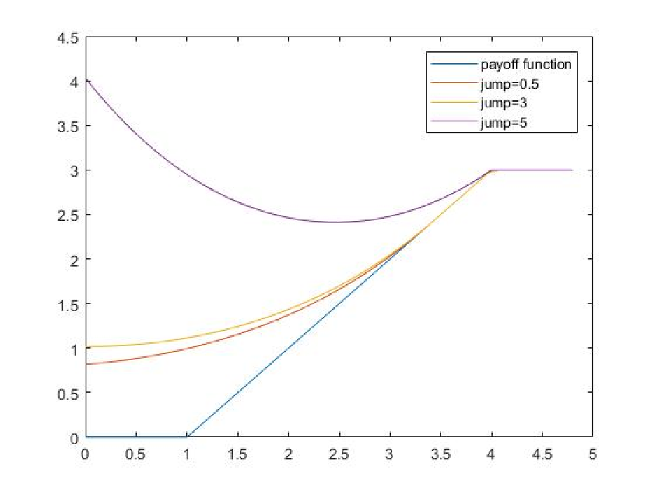
Figure 1. Value functions against initial state
Refer to caption

In Figure 1, we assume that the jump size is fixed at 0.50.5 (respectively 33 and 55) and the parameter λ=1\lambda=1. The graph shows that the value function and exercise point increases with the jump size. We can also mention that the construction of the value function by the viscosity solution can generally be used under weaker condition as compared to the smooth fit principle. Since gg is not differential, the smooth fit principle may failed for example if the jump size is equal to 55.

8.3. Regime switching boundary

In order to construct a regime switching boundary Feller diffusion, we first construct a regime switching Feller process. Let 𝒮:={1,2,…,N}\mathcal{S}:=\{1,2,\ldots,N\} be a finite discrete space, where NN is a positive integer. Let (𝒜i,D⁡(𝒜i))(\mathcal{A}_{i},D(\mathcal{A}_{i})) be the infinitesimal generators of some Feller semigroups on 𝒞0​(𝖤)\mathcal{C}_{0}(\mathsf{E}). Then, define the operator (𝒜,D⁡(𝒜))(\mathcal{A},D(\mathcal{A})) as follows:

D⁡(𝒜r​e​g​i​m​e):={u∈𝒞0​(S×𝖤);u⁡(i,⋅)∈D⁡(𝒢i)},𝒜r​e​g​i​m​e​u​(i,x):=𝒜i​ui​(x)​ for ​i∈S​ and ​x∈𝖤,\displaystyle\begin{split}D(\mathcal{A}_{regime})&:=\{u\in\mathcal{C}_{0}(S\times\mathsf{E});u(i,\cdot)\in D(\mathcal{G}_{i})\},\\ \mathcal{A}_{regime}u(i,x)&:=\mathcal{A}_{i}u_{i}(x)\mbox{ for }i\in S\mbox{ and }x\in\mathsf{E},\end{split} (8.11)

where ui​(x):=u​(i,x)u_{i}(x):=u(i,x). By Hille-Yosida theorem, the above generator is the infinitesimal generator of some Feller semigroup. In addition, define the bounded operator

ℱr​e​g​i​m​e​u​(i,x):=∑j∈Nqi​j​(x)​(u⁡(j,x)−u⁡(i,x)),\displaystyle\mathcal{F}_{regime}u(i,x):=\sum_{j\in N}q_{ij}(x)(u(j,x)-u(i,x)), (8.12)

where qi​j∈𝒞b​(𝖤)q_{ij}\in\mathcal{C}_{b}(\mathsf{E}) and qi​j≥0,i,j∈ℕq_{ij}\geq 0,\,\,i,j\in\mathbb{N}. Since ℱr​e​g​i​m​e\mathcal{F}_{regime} satisfies the positive maximum principle and ℱr​e​g​i​m​e:𝒞0​(𝖤)→𝒞0​(𝖤)\mathcal{F}_{regime}:\mathcal{C}_{0}(\mathsf{E})\rightarrow\mathcal{C}_{0}(\mathsf{E}), the operator ((,,,))((\mathcal{A}_{regime}+\mathcal{F}_{regime},D(\mathcal{A}_{regime}))) is the infinitesimal generator of some Feller semigroup.

Next, we construct a regime switching boundary Feller diffusion, that is, the boundary condition is affected by a Markov chain {Z⁡(t)}t≥0\{Z(t)\}_{t\geq 0} with the state space {1,2}\{1,2\}. The intensity matrix of the chain is given by

[−q1q1q2−q2],\begin{bmatrix}-q_{1}&q_{1}\\ q_{2}&-q_{2}\end{bmatrix},

where q1,q2>0q_{1},q_{2}>0. Let {Z⁡(t),X⁡(t)}t≥0\{Z(t),X(t)\}_{t\geq 0} be a Feller process on the state space {1,2}×[0,∞)\{1,2\}\times[0,\infty). {X⁡(t)}t≥0\{X(t)\}_{t\geq 0} is a one-side diffusion which behaves like Brownian motion in (0,∞)(0,\infty) but is modulated at 00. More precisely, when X⁡(t)X(t) touches 00, it either become a sticky Brownian motion or reflected Brownian motion. We denote by Z⁡(t)=1Z(t)=1 the state for sticky Brownian motion and Z⁡(t)=2Z(t)=2 the tate for reflected Brownian motion. Its infinitesimal generator (𝒢,D⁡(𝒢))(\mathcal{G},D(\mathcal{G})) is defined by:

D⁡(𝒢):={u∈𝒞0({1,2}×[0,∞);ui∈𝒞2([0,∞)) for i=1,2,Dx​xu(1,0)=0 and Dxu(2,0)=0},𝒢​u​(i,x):=12Dx​xu(i,x)+qiu(3−i,x)−qiu(i,x) for i=1,2 and x∈[0,∞),\displaystyle\begin{split}D(\mathcal{G})&:=\{u\in\mathcal{C}_{0}(\{1,2\}\times[0,\infty);u_{i}\in\mathcal{C}^{2}([0,\infty))\mbox{ for }i=1,2,\\ &\qquad D_{xx}u(1,0)=0\mbox{ and }D_{x}u(2,0)=0\},\\ \mathcal{G}u(i,x)&:=\frac{1}{2}D_{xx}u(i,x)+q_{i}u(3-i,x)-q_{i}u(i,x)\mbox{ for }i=1,2\mbox{ and }x\in[0,\infty),\end{split} (8.13)

where ui​(x)=u​(i,x)u_{i}(x)=u(i,x) for all (i,x)∈{1,2}×[0,∞)(i,x)\in\{1,2\}\times[0,\infty). As a consequence of Theorem 5.3, we have the following characterisation of the value function for the optimal stopping problem (8.1):

Corollary 8.4.

There exists a unique pair of viscosity solution V1,V2∈𝒞b​([0,∞))V_{1},V_{2}\in\mathcal{C}_{b}([0,\infty)) such that V1V_{1} is a viscosity solution associated with (𝒢1,D⁡(𝒢1))(\mathcal{G}_{1},D(\mathcal{G}_{1})) to

min⁡((a+q1)​w−𝒢1​w−q1​V2,w−g⁡(1,⋅))=0,\min((a+q_{1})w-\mathcal{G}_{1}w-q_{1}V_{2},w-g(1,\cdot))=0,

and V2V_{2} is a viscosity solution associated with (𝒢2,D⁡(𝒢2))(\mathcal{G}_{2},D(\mathcal{G}_{2})) to

min⁡((a+q2)​w−𝒢2​w−q2​V1,w−g⁡(2,⋅))=0.\min((a+q_{2})w-\mathcal{G}_{2}w-q_{2}V_{1},w-g(2,\cdot))=0.

Additionally, assume that u⁡(i∗,⋅)u(i^{*},\cdot) is a viscosity supersolution to

a​g​(i∗,x)−𝒢i∗​g​(i∗,x)+qi∗​(g⁡(3−i∗,x)−g⁡(i∗,x))=0, for ​x∈(x∗,∞).ag(i^{*},x)-\mathcal{G}_{i^{*}}g(i^{*},x)+q_{i^{*}}(g(3-i^{*},x)-g(i^{*},x))=0,\mbox{ for }x\in(x^{*},\infty).

Then, V⁡(i∗,x)=u⁡(i∗,x)V(i^{*},x)=u(i^{*},x) for x∈[0,x∗)x\in[0,x^{*}) and V⁡(i∗,x)=g⁡(i∗,x)V(i^{*},x)=g(i^{*},x) for x∈[x∗,∞)x\in[x^{*},\infty). Furthermore,

V⁡(3−i∗,⋅)V(3-i_{*},\cdot) is the unique viscosity solution associated with (𝒢3−i∗,D⁡(𝒢3−i∗))(\mathcal{G}_{3-i^{*}},D(\mathcal{G}_{3-i^{*}})) to

min⁡((a+q3−i∗)​w−𝒢3−i∗∗​w−q3−i∗​V​(i∗,⋅),w−g⁡(3−i∗,⋅))=0\displaystyle\min((a+q_{3-i^{*}})w-\mathcal{G}^{*}_{3-i^{*}}w-q_{3-i^{*}}V(i^{*},\cdot),w-g(3-i^{*},\cdot))=0

In order to derive explicit value function, we define fundamental solutions for optimal stopping problem. Let

uk​(i,x)\displaystyle u_{k}(i,x) =αi​k​eβk​x\displaystyle=\alpha_{ik}e^{\beta_{k}x} (8.14)
vj​(i,x)\displaystyle v_{j}(i,x) :={qi​ℛa+qi(j)​g3−i​(x)​ for ​i=jgi​(x)​ for ​i≠j,\displaystyle:=\begin{cases}q_{i}\mathcal{R}^{(j)}_{a+q_{i}}g_{3-i}(x)\text{ for }i=j\\ g_{i}(x)\text{ for }i\neq j,\end{cases} (8.15)
wj​1​(i,x)\displaystyle w_{j1}(i,x) :={eγj​x​ for ​i=j0​ for ​i≠j,\displaystyle:=\begin{cases}e^{\gamma_{j}x}\text{ for }i=j\\ 0\text{ for }i\neq j,\end{cases} (8.16)
wj​2​(i,x)\displaystyle w_{j2}(i,x) :={e−γj​x​ for ​i=j0​ for ​i≠j,\displaystyle:=\begin{cases}e^{-\gamma_{j}x}\text{ for }i=j\\ 0\text{ for }i\neq j,\end{cases} (8.17)

where i,j=1,2i,j=1,2, k=1,2,3,4k=1,2,3,4 β1=2​a\beta_{1}=\sqrt{2a}, β2=−2​a\beta_{2}=-\sqrt{2a}, β3=2​(a+q1+q2CLOSE\beta_{3}=\sqrt{2(a+q_{1}+q_{2}} and β4=−2​(a+q1+q2)\beta_{4}=-\sqrt{2(a+q_{1}+q_{2})}, α1​k=1\alpha_{1k}=1 and α2​k=q1a+q1−12​zj2\alpha_{2k}=\frac{q_{1}}{a+q_{1}-\frac{1}{2}z_{j}^{2}} and γj=2​(a+qj)\gamma_{j}=\sqrt{2(a+q_{j})}.

Lemma 8.5.

The following hold for j=1,2j=1,2:

  1. (1)

    For any Aj∈ℝA_{j}\in\mathbb{R}, u:=∑j=14Aj​uju:=\sum_{j=1}^{4}A_{j}u_{j} is a solution to

    a​u​(i,x)−𝒢∗​u​(i,x)=0​ for ​(i,x)∈{1,2}×(0,∞)\displaystyle au(i,x)-\mathcal{G}^{*}u(i,x)=0\text{ for }(i,x)\in\{1,2\}\times(0,\infty) (8.18)
  2. (2)

    For any Bk∈ℝB_{k}\in\mathbb{R}, w:=∑k=12Bk​wj​k+vjw:=\sum_{k=1}^{2}B_{k}w_{jk}+v_{j} is a solution to

    a​w​(i,x)−𝒢∗​w​(i,x)=0​ for ​(i,x)∈{j}×(0,∞),\displaystyle aw(i,x)-\mathcal{G}^{*}w(i,x)=0\text{ for }(i,x)\in\{j\}\times(0,\infty), (8.19)
Proof.

The result simply follows from direct computations given the parameters. ∎

The subsequent result can be seen as a verification theorem for the value function.

Proposition 8.6.

Assume that there exist 0≤x1∗≤x2∗<∞0\leq x_{1}^{*}\leq x_{2}^{*}<\infty, Aj∈ℝA_{j}\in\mathbb{R}, Bk∈ℝB_{k}\in\mathbb{R} for j=1,2,3,4j=1,2,3,4 and k=1,2k=1,2 such that the function

u⁡(i,x):={∑j=14Aj​uj​(i,x)​ for ​(i,x)∈{1,2}×[0,x1∗),∑k=12Bk​wj​k+vj​ for ​{1,2}×[x1∗,x2∗),g⁡(i,x)​ for ​{1,2}×[x2∗,∞),\displaystyle u(i,x):=\begin{cases}\sum_{j=1}^{4}A_{j}u_{j}(i,x)\text{ for }(i,x)\in\{1,2\}\times[0,x_{1}^{*}),\\ \sum_{k=1}^{2}B_{k}w_{jk}+v_{j}\text{ for }\{1,2\}\times[x_{1}^{*},x_{2}^{*}),\\ g(i,x)\text{ for }\{1,2\}\times[x_{2}^{*},\infty),\end{cases} (8.20)

satisfies

  1. (1)

    u≥gu\geq g,

  2. (2)

    u∈𝒞b​({1,2}×[0,∞)CLOSEu\in\mathcal{C}_{b}(\{1,2\}\times[0,\infty),

  3. (3)

    uu is a viscosity solution to

    min⁡(a​u​(i,x)−𝒢∗​u​(i,0),u⁡(i,x)−g⁡(i,x))=0​ for ​(i,x)∈{(1,0),(2,0),(j,x1∗)}\displaystyle\min(au(i,x)-\mathcal{G}^{*}u(i,0),u(i,x)-g(i,x))=0\text{ for }(i,x)\in\{(1,0),(2,0),(j,x_{1}^{*})\} (8.21)
  4. (4)

    uu is a viscosity supersolution to

    a​u​(i,x)−𝒢∗​u​(i,x)=0​ for ​(i,x)∈{j}×[x2∗,∞)∪{3−j}×[x1∗,∞)\displaystyle au(i,x)-\mathcal{G}^{*}u(i,x)=0\text{ for }(i,x)\in\{j\}\times[x_{2}^{*},\infty)\cup\{3-j\}\times[x_{1}^{*},\infty) (8.22)

Then, the value function V=uV=u.

Proof.

To show that uu is the viscosity solution, we divide the state space into 3 cases,

  1. (i)

    For (i,x)∈{1,2}×(0,x1∗)∪{j}×(x1∗,x2∗)(i,x)\in\{1,2\}\times(0,x_{1}^{*})\cup\{j\}\times(x_{1}^{*},x_{2}^{*}) , the viscosity property is given by Lemma 8.5

  2. (ii)

    For (i,x)∈{(1,0),(2,0),(j,x1∗)}(i,x)\in\{(1,0),(2,0),(j,x_{1}^{*})\}, the viscosity property follows from condition (3)

  3. (iii)

    For (i,x)∈{j}×[x2∗,∞)∪{3−j}×[x1∗,∞)(i,x)\in\{j\}\times[x_{2}^{*},\infty)\cup\{3-j\}\times[x_{1}^{*},\infty), the viscosity property follows from condition (1) and condition (4).

∎

Using Proposition 8.6, we need to find Aj,j=1,2,3,4,Bk,k=1,2,x1∗A_{j},\,j=1,2,3,4,B_{k},\,k=1,2,\,x_{1}^{*} and x2∗x_{2}^{*} such that the viscosity property is satisfied at the following 55 points; {(1,0),(2,0),(1,x1∗),(1,x2∗),(2,x1∗)}\{(1,0),(2,0),(1,x_{1}^{*}),(1,x_{2}^{*}),(2,x_{1}^{*})\} (respectively {(1,0),(2,0),(2,x1∗),(2,x2∗),(1,x1∗)}\{(1,0),(2,0),(2,x_{1}^{*}),(2,x_{2}^{*}),(1,x_{1}^{*})\}), and the continuity property is satisfied at the following 33 points {(1,x1∗),(1,x2∗),(2,x1∗)}\{(1,x_{1}^{*}),(1,x_{2}^{*}),(2,x_{1}^{*})\} (respectively {(2,x1∗),(2,x2∗),(1,x1∗)}\{(2,x_{1}^{*}),(2,x_{2}^{*}),(1,x_{1}^{*})\}).

We can then derive the explicit expression of the value function as follows:

Corollary 8.7.

Let AjA_{j}, BkB_{k}, c1<x1∗<x2∗≤c2c_{1}<x_{1}^{*}<x_{2}^{*}\leq c_{2}, l∈{1,2}l\in\{1,2\} such that

{∑jAj​ux​(1,0)=0,∑jAj​ux​x​(2,0)=0,∑jAj​uj​(l,x1∗)=∑kBk​wl​k​(1,x1∗)+vl​(x1∗),∑jAj​uj​(3−l,x1∗)=g⁡(3−l,x1∗),∑kBkwl​k(,x2∗)+v3−l(x2∗)=g(l,x2∗),∑jAj​(uj)x​(l,x1∗)=∑kBk​(wl​k)x​(1,x1∗)+(vl)x​(x1∗)\displaystyle\begin{cases}\sum_{j}A_{j}u_{x}(1,0)=0,\\ \sum_{j}A_{j}u_{xx}(2,0)=0,\\ \sum_{j}A_{j}u_{j}(l,x_{1}^{*})=\sum_{k}B_{k}w_{lk}(1,x_{1}^{*})+v_{l}(x_{1}^{*}),\\ \sum_{j}A_{j}u_{j}(3-l,x_{1}^{*})=g(3-l,x_{1}^{*}),\\ \sum_{k}B_{k}w_{lk}(,x_{2}^{*})+v_{3-l}(x_{2}^{*})=g(l,x_{2}^{*}),\\ \sum_{j}A_{j}(u_{j})_{x}(l,x_{1}^{*})=\sum_{k}B_{k}(w_{lk})_{x}(1,x_{1}^{*})+(v_{l})_{x}(x_{1}^{*})\end{cases} (8.23)

and ∑jAj​uj−g\sum_{j}A_{j}u_{j}-g has a local minimum at (3−l,x1∗)(3-l,x_{1}^{*}) and ∑jBk​uk+vl−g\sum_{j}B_{k}u_{k}+v_{l}-g has a local minimum at (l,x2∗)(l,x_{2}^{*}). If u≥gu\geq g, then uu is the value function.

For fixed numerical values of c1,c2,q1,q2,c_{1},c_{2},q_{1},q_{2}, and aa, we show in the next example that we can find the above parameters Aj,j=1,2,3,4,Bk,k=1,2,x1∗A_{j},\,j=1,2,3,4,B_{k},\,k=1,2,\,x_{1}^{*} and x2∗x_{2}^{*} and thus derive the value function.

Assume that a=0.1a=0.1. Figure 2 depicts the evolution of the value functions

V⁡(x)=supτ𝑬i,x​[e−a​τ​{(X⁡(t)−c1)+−(X⁡(t)−c2)+}],\displaystyle V(x)=\sup_{\tau}\mbox{\boldmath$E$}^{i,x}\Big[e^{-a\tau}\Big\{(X(t)-c_{1})^{+}-(X(t)-c_{2})^{+}\Big\}\Big], (8.24)

where c1=1c_{1}=1 and c2=4c_{2}=4 for regime switching diffusion with reflected boundary and sticky boundary with the intensity matrix

[−q1q1q2−q2]=[−0.10.10.1−0.1],\displaystyle\begin{bmatrix}-q_{1}&q_{1}\\ q_{2}&-q_{2}\end{bmatrix}=\begin{bmatrix}-0.1&0.1\\ 0.1&-0.1\end{bmatrix},

where state 1 represents the reflected boundary and state 2 represents the sticky boundary.
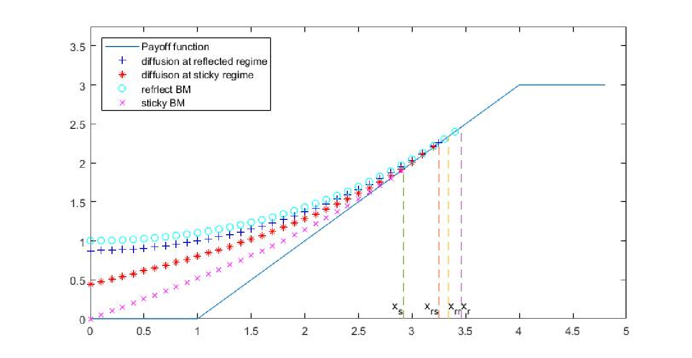
Figure 2. Value functions against initial state
Refer to caption

xsx_{s}, xr​sx_{rs}, xr​rx_{rr} and xrx_{r} are the exercise points in the cases of sticky Brownian motion, diffusion at sticky regime, diffusion at reflected regime and reflected Brownian motion, respectively. Figure 2 depicts the evolution of the value function of reflected Brownian motion and sticky Brownian motion with regime switching respectively. The sticky Brownian motion has an absorbing point at 00 and the payoff function at 00 equals 00. This means that the value function of the optimal stopping problem for sticky Brownian motion at 00 is 00 which is smaller than that of the reflected Brownian motion at 00. Therefore, the exercise points xrx_{r} for reflected Brownian motion is larger than that of the sticky Brownian motion xsx_{s}. The graph also shows that the value function of this regime switching process will stay between the above two value functions. This is in line with the intuition. Additionally, the graph shows that the exercise points xr​sx_{rs} and xr​rx_{rr} are between xsx_{s} and xrx_{r}.

Appendix A Proof of Theorem 2.11

(1) We first prove (1) in Theorem 2.11, that is, there exists a unique solution vλ∈D⁡(ℒ)v_{\lambda}\in D(\mathcal{L}) to (2.7) for each λ>0\lambda>0. Define the penalty function vλv_{\lambda} as the solution to

vλ=ℛa​(f+λ​(g−vλ)+).v_{\lambda}=\mathcal{R}_{a}(f+\lambda(g-v_{\lambda})^{+}). (A.1)

We start by showing that (A.1) has a unique solution in 𝒞0​(𝖤)\mathcal{C}_{0}(\mathsf{E}) in the following lemma.

Lemma A.1.

Suppose Assumption 2.10 holds. For any λ>0\lambda>0, (A.1) admits a unique solution vλ∈𝒞0​(𝖤)v_{\lambda}\in\mathcal{C}_{0}({\mathsf{E}}). Additionally, the solution to (A.1) is equivalent to the solution to the following equation

vλ=ℛa+λ​(f+λ​(g−vλ)++λ​vλ).v_{\lambda}=\mathcal{R}_{a+\lambda}(f+\lambda(g-v_{\lambda})^{+}+\lambda v_{\lambda}). (A.2)

(Equivalence here means that, the solution to one is also a solution to the other, vice versa.)

Proof.

We first show that the solution to (A.1) is equivalent to the solution to (A.2). Let vλv_{\lambda} be the solution to (A.1) in 𝒞0​(𝖤)\mathcal{C}_{0}(\mathsf{E}). Using the resolvent identity equation (2.2), we obtain

ℛa+λ​(f+λ​(g−vλ)+)−ℛa​(f+λ​(g−vλ)+)=−λ​ℛa+λ​ℛa​(f+λ​(g−vλ)+).\displaystyle\mathcal{R}_{a+\lambda}(f+\lambda(g-v_{\lambda})^{+})-\mathcal{R}_{a}(f+\lambda(g-v_{\lambda})^{+})=-\lambda\mathcal{R}_{a+\lambda}\mathcal{R}_{a}(f+\lambda(g-v_{\lambda})^{+}). (A.3)

Combining (A.1) and (A.3), we have

ℛa+λ​(f+λ​(g−vλ)+)−vλ=−λ​ℛa+λ​vλ.\mathcal{R}_{a+\lambda}(f+\lambda(g-v_{\lambda})^{+})-v_{\lambda}=-\lambda\mathcal{R}_{a+\lambda}v_{\lambda}.

Therefore, vλv_{\lambda} is also a solution to (A.2).
Now, let vλv_{\lambda} be a solution to (A.2). Using once more (2.2), we have

ℛa+λ​(f+λ​(g−vλ)++λ​vλ)−ℛa​(f+λ​(g−vλ)++λ​vλ)\displaystyle\mathcal{R}_{a+\lambda}(f+\lambda(g-v_{\lambda})^{+}+\lambda v_{\lambda})-\mathcal{R}_{a}(f+\lambda(g-v_{\lambda})^{+}+\lambda v_{\lambda})
=\displaystyle= −λ​ℛa​ℛa+λ​(f+λ​(g−vλ)++λ​vλ).\displaystyle-\lambda\mathcal{R}_{a}\mathcal{R}_{a+\lambda}(f+\lambda(g-v_{\lambda})^{+}+\lambda v_{\lambda}). (A.4)

Combining (A.2) and (A.4) yields

vλ−ℛa​(f+λ​(g−vλ)++λ​vλ)=−λ​ℛa​vλ.v_{\lambda}-\mathcal{R}_{a}(f+\lambda(g-v_{\lambda})^{+}+\lambda v_{\lambda})=-\lambda\mathcal{R}_{a}v_{\lambda}.

Hence, vλv_{\lambda} is also a solution to (A.1).

In order to complete the proof, it is enough to show that (A.2) has the unique solution. Define a new operator 𝒵\mathcal{Z} as follows:

𝒵​w:=ℛa+λ​(f+λ​(g−w)++λ​w).\mathcal{Z}w:=\mathcal{R}_{a+\lambda}(f+\lambda(g-w)^{+}+\lambda w).

We have that f,g∈𝒞0​(𝖤)f,g\in\mathcal{C}_{0}(\mathsf{E}) and the resolvent operator maps from 𝒞0​(𝖤)\mathcal{C}_{0}(\mathsf{E}) to 𝒞0​(𝖤)\mathcal{C}_{0}(\mathsf{E}). Let w∈𝒞0​(𝖤)w\in\mathcal{C}_{0}(\mathsf{E}), then 𝒵​w\mathcal{Z}w is also in 𝒞0​(𝖤)\mathcal{C}_{0}(\mathsf{E}). Furthermore, let w1,w2∈𝒞0​(𝖤)w_{1},w_{2}\in\mathcal{C}_{0}{(\mathsf{E})}. Using the linearity of the resolvent and the fact that (g−wi)++wi=max⁡(g,wi)(g-w_{i})^{+}+w_{i}=\max(g,w_{i}) for i=1,2i=1,2, we have

‖𝒵​w1−𝒵​w2‖∞\displaystyle\|\mathcal{Z}w_{1}-\mathcal{Z}w_{2}\|_{\infty} =\displaystyle= ‖ℛa+λ​(f+λ​(g−w1)++λ​w1)−ℛa+λ​(f+λ​(g−w2)++λ​w2)‖∞\displaystyle\|\mathcal{R}_{a+\lambda}(f+\lambda(g-w_{1})^{+}+\lambda w_{1})-\mathcal{R}_{a+\lambda}(f+\lambda(g-w_{2})^{+}+\lambda w_{2})\|_{\infty}
=\displaystyle= ‖λ​ℛa+λ​(max⁡(g,w1)−max⁡(g,w2))‖∞\displaystyle\|\lambda\mathcal{R}_{a+\lambda}(\max{(g,w_{1})}-\max{(g,w_{2})})\|_{\infty}
≤\displaystyle\leq λa+λ∥max(g,w1)−max(g,w2))∥∞\displaystyle\frac{\lambda}{a+\lambda}\|\max{(g,w_{1})}-\max{(g,w_{2})})\|_{\infty}
≤\displaystyle\leq λa+λ​‖w1−w2‖∞,\displaystyle\frac{\lambda}{a+\lambda}\|w_{1}-w_{2}\|_{\infty},

where the inequality comes from (2.4). Hence, 𝒵\mathcal{Z} is a contraction mapping from 𝒞0​(𝖤)\mathcal{C}_{0}(\mathsf{E}) to 𝒞0​(𝖤)\mathcal{C}_{0}(\mathsf{E}). By Banach fixed point theorem, the equation w=𝒵​ww=\mathcal{Z}w (which is the same as (A.2)) has a unique solution w∈𝒞0​(𝖤)w\in\mathcal{C}_{0}(\mathsf{E}), that we denote by vλv_{\lambda}. ∎

Recall that the operator (λ−ℒ)(\lambda-\mathcal{L}) is a bijection of D⁡(ℒ)D(\mathcal{L}) to 𝒞0​(𝖤)\mathcal{C}_{0}(\mathsf{E}) and its inverse is the resolvent ℛλ\mathcal{R}_{\lambda} (see Corollary 2.8). The solution to (A.1) is equivalent to the solution to (2.7). It remains to show that vλ∈D⁡(ℒ)v_{\lambda}\in D(\mathcal{L}). We have shown that (A.1) has the unique solution vλv_{\lambda} in 𝒞0​(𝖤)\mathcal{C}_{0}(\mathsf{E}) such that f+λ​(g−w)+∈𝒞0​(𝖤)f+\lambda(g-w)^{+}\in\mathcal{C}_{0}(\mathsf{E}). Therefore, (1) in Theorem 2.11 is proved.

(2) Let vλv_{\lambda} be the unique solution in D⁡(ℒ)D(\mathcal{L}) to (2.7) for λ>0\lambda>0. We prove that the sequence of penalty functions {vλ}λ>0\{v_{\lambda}\}_{\lambda>0} converges uniformly to the value function VV in 𝒞0​(𝖤)\mathcal{C}_{0}(\mathsf{E}) as λ→∞\lambda\rightarrow\infty. We need the following two preliminary lemmas.

Lemma A.2.

Suppose Assumption 2.10 holds. Let {gn}n​ℕ+\{g_{n}\}_{n\mathbb{N}^{+}} be a sequence in 𝒞0​(𝖤)\mathcal{C}_{0}(\mathsf{E}) such that

‖g−gn‖∞≤1n.\displaystyle\|g-g_{n}\|_{\infty}\leq\frac{1}{n}. (A.5)

Define a sequence of the corresponding value functions {Vn}n∈ℕ+\{V_{n}\}_{n\in\mathbb{N}^{+}} by

Vn​(x):=supτ∈𝒯Jx(n)​(τ)​ for ​x∈𝖤​ and ​n∈ℕ+,V_{n}(x):=\sup_{\tau\in\mathcal{T}}J^{(n)}_{x}(\tau)\text{ for }x\in\mathsf{E}\text{ and }n\in\mathbb{N}^{+}, (A.6)

where Jx(n)​(τ)=𝐄x​[∫0τe−a​s​f​(X⁡(s))​𝑑s+e−a​τ​gn​(X⁡(τ))].J^{(n)}_{x}(\tau)=\mbox{\boldmath$E$}^{x}\left[\int_{0}^{\tau}{e^{-as}f(X(s))ds}+e^{-a\tau}g_{n}(X(\tau))\right]. Then, VnV_{n} converges to VV defined by (2.6) uniformly as n→∞n\rightarrow\infty.

Proof.

Let x∈𝖤x\in\mathsf{E}, n∈ℕ+n\in\mathbb{N}^{+} and ε>0\varepsilon>0. Define a ε\varepsilon-optimal stopping time τε∗\tau_{\varepsilon}^{*} such that

V⁡(x)−ε≤Jx​(τε∗).V(x)-\varepsilon\leq J_{x}(\tau_{\varepsilon}^{*}). (A.7)

Therefore, we have

V⁡(x)\displaystyle V(x) ≤𝑬x​[∫0τε∗e−a​s​f​(X⁡(s))​𝑑s+e−a​τε∗​g​(X⁡(τε∗))]+ε\displaystyle\leq\mbox{\boldmath$E$}^{x}\bigg[\int_{0}^{\tau_{\varepsilon}^{*}}e^{-as}f(X(s))ds+e^{-a\tau_{\varepsilon}^{*}}g(X(\tau_{\varepsilon}^{*}))\bigg]+\varepsilon
≤𝑬x​[∫0τε∗e−a​s​f​(X⁡(s))​𝑑s+e−a​τε∗​(gn​(X⁡(τε∗))+‖g−gn‖∞)]+ε\displaystyle\leq\mbox{\boldmath$E$}^{x}\bigg[\int_{0}^{\tau_{\varepsilon}^{*}}e^{-as}f(X(s))ds+e^{-a\tau_{\varepsilon}^{*}}(g_{n}(X(\tau_{\varepsilon}^{*}))+\|g-g_{n}\|_{\infty})\bigg]+\varepsilon
≤Jx(n)​(τε∗)+1n+ε≤Vn​(x)+1n+ε.\displaystyle\leq J_{x}^{(n)}(\tau_{\varepsilon}^{*})+\frac{1}{n}+\varepsilon\leq V_{n}(x)+\frac{1}{n}+\varepsilon.

Since ε\varepsilon is an arbitrary positive constant, V⁡(x)−Vn​(x)≤1nV(x)-V_{n}(x)\leq\frac{1}{n}. On the other hand, we can find a stopping time τε∗(n)\tau_{\varepsilon}^{*(n)} for VnV_{n} such that Vn​(x)−ε≤Jx(n)​(τε∗(n)).V_{n}(x)-\varepsilon\leq J^{(n)}_{x}(\tau_{\varepsilon}^{*(n)}). One also obtains Vn​(x)−V⁡(x)≤1nV_{n}(x)-V(x)\leq\frac{1}{n} similarly. Therefore, we have

‖V−Vn‖∞≤1n.\displaystyle\|V-V_{n}\|_{\infty}\leq\frac{1}{n}. (A.8)

Then, the proof is completed. ∎

Lemma A.3.

Suppose Assumption 2.10 holds. Let vλv_{\lambda} be the solution to (A.1) for each λ>0\lambda>0. Then, vλv_{\lambda} satisfies

vλ​(x)=supτ𝑬x​[∫0τe−a​s​f​(X⁡(s))​𝑑s+e−a​τ​(g−(g−vλ)+)​(X⁡(τ))].v_{\lambda}(x)=\sup_{\tau}\mbox{\boldmath$E$}^{x}\bigg[\int_{0}^{\tau}{e^{-as}f(X(s))ds}+e^{-a\tau}(g-(g-v_{\lambda})^{+})(X(\tau))\bigg]. (A.9)

Additionally, V≥vλV\geq v_{\lambda}.

Proof.

Let x∈𝖤x\in\mathsf{E}, λ>0\lambda>0 and τ\tau be a ℱt\mathcal{F}_{t}-stopping time. We know from (1) in Theorem 2.11 that vλ∈D⁡(ℒ)v_{\lambda}\in D(\mathcal{L}). Using Dynkin’s formula and optional stopping theorem,

vλ​(x)\displaystyle v_{\lambda}(x) =𝑬x​[∫0τe−a​s​(f⁡(X⁡(s))+λ​(g−vλ)+​(X⁡(s)))​𝑑s+e−a​τ​vλ​(X⁡(τ))].\displaystyle=\mbox{\boldmath$E$}^{x}\Big[\int_{0}^{\tau}{e^{-as}(f(X(s))+\lambda(g-v_{\lambda})^{+}(X(s)))ds}+e^{-a\tau}v_{\lambda}(X(\tau))\Big]. (A.10)
≥𝑬x​[∫0τe−a​s​f​(X⁡(s))​𝑑s+e−a​τ​(g−(g−vλ)+)​(X⁡(τ))].\displaystyle\geq\mbox{\boldmath$E$}^{x}\bigg[\int_{0}^{\tau}{e^{-as}f(X(s))ds}+e^{-a\tau}(g-(g-v_{\lambda})^{+})(X(\tau))\bigg].

Taking the supremum on both sides, we obtain

vλ​(x)≥supτ𝑬x​[∫0τe−a​s​f​(X⁡(s))​𝑑s+e−a​τ​(g−(g−vλ)+)​(X⁡(τ))].v_{\lambda}(x)\geq\sup_{\tau}\mbox{\boldmath$E$}^{x}\Big[\int_{0}^{\tau}{e^{-as}f(X(s))ds}+e^{-a\tau}(g-(g-v_{\lambda})^{+})(X(\tau))\Big]. (A.11)

In order to prove the equality, define the stopping time σ∗\sigma^{*} by σ∗:=inf{s≥0;vλ​(X⁡(s))≤g⁡(X⁡(s))}\sigma^{*}:=\inf\{s\geq 0;\;v_{\lambda}(X(s))\leq g(X(s))\}. Since {X⁡(t)}t≥0\{X(t)\}_{t\geq 0} is right continuous and vλv_{\lambda} and gg are continuous, we have vλ​(X⁡(σ∗))≤g⁡(X⁡(σ∗))v_{\lambda}(X(\sigma^{*}))\leq g(X(\sigma^{*})). Using the preceding and (A.10), we have

vλ​(x)\displaystyle v_{\lambda}(x) =𝑬x​[∫0σ∗e−a​s​(f⁡(X⁡(s))+λ​(g−vλ)+​(X⁡(s)))​𝑑s+e−a​σ∗​vλ​(X⁡(σ∗))]\displaystyle=\mbox{\boldmath$E$}^{x}\Big[\int_{0}^{\sigma^{*}}{e^{-as}(f(X(s))+\lambda(g-v_{\lambda})^{+}(X(s)))ds}+e^{-a\sigma^{*}}v_{\lambda}(X(\sigma^{*}))\Big]
=𝑬x[∫0σ∗e−a​sf(X(s)ds+e−a​σ∗(g−(g−vλ)+)(X(σ∗))].\displaystyle=\mbox{\boldmath$E$}^{x}\Big[\int_{0}^{\sigma^{*}}{e^{-as}f(X(s)ds}+e^{-a\sigma^{*}}(g-(g-v_{\lambda})^{+})(X(\sigma^{*}))\Big].

Hence, (A.9) is proved. Furthermore, since g−(g−vλ)+≤gg-(g-v_{\lambda})^{+}\leq g, (A.9) implies V≥vλV\geq v_{\lambda} for all λ>0\lambda>0. The proof is completed. ∎

Lemma A.4.

Suppose Assumption 2.10 holds. Assume in addition that g∈D⁡(ℒ)g\in D(\mathcal{L}). Let vλv_{\lambda} be the solution to (2.7) for λ>0\lambda>0. vλv_{\lambda} converges to VV uniformly as λ→∞\lambda\to\infty and hence V∈𝒞0​(𝖤)V\in\mathcal{C}_{0}(\mathsf{E}).

Proof.

Let x∈𝖤x\in\mathsf{E} and λ>0\lambda>0. Using (A.9), we get

vλ​(x)\displaystyle v_{\lambda}(x) =supτ𝑬x​[∫0τe−a​s​f​(X⁡(s))​𝑑s+e−a​τ​(g−(g−vλ)+)​(X⁡(τ))]\displaystyle=\sup_{\tau}{\mbox{\boldmath$E$}^{x}\Big[\int_{0}^{\tau}{e^{-as}f(X(s))ds}+e^{-a\tau}(g-(g-v_{\lambda})^{+})(X(\tau))\Big]}
≥supτ𝑬x​[∫0τe−a​s​f​(X⁡(s))​𝑑s+e−a​τ​g​(X⁡(τ))]−supτ𝑬x​[e−a​τ​(g−vλ)+​(X⁡(τ))]\displaystyle\geq\sup_{\tau}{\mbox{\boldmath$E$}^{x}\Big[\int_{0}^{\tau}{e^{-as}f(X(s))ds}+e^{-a\tau}g(X(\tau))\Big]}-\sup_{\tau}{\mbox{\boldmath$E$}^{x}\Big[e^{-a\tau}(g-v_{\lambda})^{+}(X(\tau))\Big]}
≥V⁡(x)−supτ𝑬x​[(g−vλ)+​(X⁡(τ))]\displaystyle\geq V(x)-\sup_{\tau}{\mbox{\boldmath$E$}^{x}\left[(g-v_{\lambda})^{+}(X(\tau))\right]}
≥V⁡(x)−‖(g−vλ)+‖∞.\displaystyle\geq V(x)-\|(g-v_{\lambda})^{+}\|_{\infty}.

Additionally, we have from Lemma A.3 that V≥vλV\geq v_{\lambda} for all λ>0\lambda>0. Then,

‖V−vλ‖∞≤‖(g−vλ)+‖∞.\|V-v_{\lambda}\|_{\infty}\leq\|(g-v_{\lambda})^{+}\|_{\infty}. (A.12)

Furthermore, since vλ∈D⁡(ℒ)v_{\lambda}\in D(\mathcal{L}) by (1) in Theorem 2.11, g−vλ∈D⁡(ℒ)g-v_{\lambda}\in D(\mathcal{L}) and thus

g−vλ=ℛa​((a−ℒ)​(g−vλ)).g-v_{\lambda}=\mathcal{R}_{a}((a-\mathcal{L})(g-v_{\lambda})).

Hence, using (2.7) and similar argument as in (A.3), we get

g−vλ\displaystyle g-v_{\lambda} =ℛa​((a−ℒ)​g−(a−ℒ)​vλ)\displaystyle=\mathcal{R}_{a}((a-\mathcal{L})g-(a-\mathcal{L})v_{\lambda})
=ℛa​((a−ℒ)​g−f−λ​(g−vλ)+)\displaystyle=\mathcal{R}_{a}((a-\mathcal{L})g-f-\lambda(g-v_{\lambda})^{+})
=ℛa+λ​((a−ℒ)​g−f−λ​(g−vλ)++λ⁡(g−vλ))\displaystyle=\mathcal{R}_{a+\lambda}((a-\mathcal{L})g-f-\lambda(g-v_{\lambda})^{+}+\lambda(g-v_{\lambda}))
≤ℛa+λ​((a−ℒ)​g−f−λ​(g−vλ)++λ​(g−vλ)+)\displaystyle\leq\mathcal{R}_{a+\lambda}((a-\mathcal{L})g-f-\lambda(g-v_{\lambda})^{+}+\lambda(g-v_{\lambda})^{+}) (A.13)
≤‖(a−ℒ)​g−f‖∞a+λ.\displaystyle\leq\frac{\|(a-\mathcal{L})g-f\|_{\infty}}{a+\lambda}.

Thus, it follows from (A.12) that

‖V−vλ‖∞≤‖(g−vλ)+‖∞≤‖(a−ℒ)​g−f‖∞a+λ≤Ma+λ,\displaystyle\|V-v_{\lambda}\|_{\infty}\leq\|(g-v_{\lambda})^{+}\|_{\infty}\leq\frac{\|(a-\mathcal{L})g-f\|_{\infty}}{a+\lambda}\leq\frac{M}{a+\lambda}, (A.14)

where M>0M>0 is a constant. Hence, vλv_{\lambda} converges to VV uniformly as λ→∞\lambda\rightarrow\infty. The proof of (1) in Theorem 2.11 is completed. ∎

It remains to show that the conclusion of Lemma A.4 is also true for any g∈𝒞0​(𝖤)g\in\mathcal{C}_{0}(\mathsf{E}). Let g∈𝒞0​(𝖤)g\in\mathcal{C}_{0}(\mathsf{E}). D⁡(ℒ)D(\mathcal{L}) is dense in 𝒞0​(𝖤)\mathcal{C}_{0}(\mathsf{E}) (see Theorem 2.7). Thus there exists a sequence {gn}n∈ℕ+\{g_{n}\}_{n\in\mathbb{N}^{+}} in D⁡(ℒ)D(\mathcal{L}) uniformly converging to gg as n→∞n\rightarrow\infty such that ‖gn−g‖∞≤1/n\|g_{n}-g\|_{\infty}\leq 1/n for any n∈ℕ+n\in\mathbb{N}^{+}. Using Lemma A.4, the sequence of the value functions {Vn}n∈ℕ+\{V_{n}\}_{n\in\mathbb{N}^{+}} defined by (A.6) is in 𝒞0​(𝖤)\mathcal{C}_{0}(\mathsf{E}). Using Lemma A.2, {Vn}n∈ℕ+\{V_{n}\}_{n\in\mathbb{N}^{+}} converges to VV uniformly as n→∞n\rightarrow\infty. Therefore, V∈𝒞0​(𝖤)V\in\mathcal{C}_{0}(\mathsf{E}).

Moreover, let vn,λv_{n,\lambda} be the solution to (2.7) after replacing gg by gng_{n} for each n∈ℕ+n\in\mathbb{N}^{+}. We prove that vn,λv_{n,\lambda} converges to vλv_{\lambda} uniformly as n→∞n\rightarrow\infty. Using (A.2),

vn,λ−vλ\displaystyle v_{n,\lambda}-v_{\lambda} =ℛa+λ​(f+λ​(gn−vn,λ)++λ​vn,λ)−ℛa+λ​(f+λ​(g−vλ)++λ​vλ)\displaystyle=\mathcal{R}_{a+\lambda}(f+\lambda(g_{n}-v_{n,\lambda})^{+}+\lambda v_{n,\lambda})-\mathcal{R}_{a+\lambda}(f+\lambda(g-v_{\lambda})^{+}+\lambda v_{\lambda})
=λ​ℛa+λ​(max⁡(gn,vn,λ)−max⁡(g,vλ))\displaystyle=\lambda\mathcal{R}_{a+\lambda}(\max(g_{n},v_{n,\lambda})-\max(g,v_{\lambda}))
≤λ​ℛa+λ​(max⁡(gn−g,vn,λ−vλ))\displaystyle\leq\lambda\mathcal{R}_{a+\lambda}(\max(g_{n}-g,v_{n,\lambda}-v_{\lambda}))
≤λa+λ​‖max⁡(gn−g,vn,λ−vλ)‖∞\displaystyle\leq\frac{\lambda}{a+\lambda}\|\max(g_{n}-g,v_{n,\lambda}-v_{\lambda})\|_{\infty}
≤λa+λ​max⁡(‖g−gn‖∞,‖vn,λ−vλ‖∞).\displaystyle\leq\frac{\lambda}{a+\lambda}\max(\|g-g_{n}\|_{\infty},\|v_{n,\lambda}-v_{\lambda}\|_{\infty}).

Similarly, we also have

vλ−vn,λ\displaystyle v_{\lambda}-v_{n,\lambda} =ℛa+λ​(f+λ​(g−vλ)++λ​vλ)−ℛa+λ​(f+λ​(gn−vn,λ)++λ​vn,λ)\displaystyle=\mathcal{R}_{a+\lambda}(f+\lambda(g-v_{\lambda})^{+}+\lambda v_{\lambda})-\mathcal{R}_{a+\lambda}(f+\lambda(g_{n}-v_{n,\lambda})^{+}+\lambda v_{n,\lambda})
≤λa+λ​max⁡(‖g−gn‖∞,‖vn,λ−vλ‖∞).\displaystyle\leq\frac{\lambda}{a+\lambda}\max(\|g-g_{n}\|_{\infty},\|v_{n,\lambda}-v_{\lambda}\|_{\infty}).

Thus

‖vλ−vn,λ‖∞≤λa+λ​max⁡(‖g−gn‖∞,‖vn,λ−vλ‖∞).\displaystyle\|v_{\lambda}-v_{n,\lambda}\|_{\infty}\leq\frac{\lambda}{a+\lambda}\max(\|g-g_{n}\|_{\infty},\|v_{n,\lambda}-v_{\lambda}\|_{\infty}).

Since λa+λ<1\frac{\lambda}{a+\lambda}<1, it follows that

‖vn,λ−vλ‖∞≤‖gn−g‖∞≤1n.\displaystyle\|v_{n,\lambda}-v_{\lambda}\|_{\infty}\leq\|g_{n}-g\|_{\infty}\leq\frac{1}{n}. (A.15)

Then, vn,λv_{n,\lambda} converges to vλv_{\lambda} uniformly as n→∞n\rightarrow\infty.

Now, let ε>0\varepsilon>0 and choose an integer n0>4εn_{0}>\frac{4}{\varepsilon}. Hence, combing (A.8), (A.14) and (A.15) yields

‖V−vλ‖∞\displaystyle\|V-v_{\lambda}\|_{\infty} ≤‖V−Vn0‖∞+‖vn0,λ−vλ‖∞+‖V−vn0,λ‖∞\displaystyle\leq\|V-V_{n_{0}}\|_{\infty}+\|v_{n_{0},\lambda}-v_{\lambda}\|_{\infty}+\|V-v_{n_{0},\lambda}\|_{\infty}
≤1n0+1n0+Mn0a+λ≤ε2+Mn0a+λ,\displaystyle\leq\frac{1}{n_{0}}+\frac{1}{n_{0}}+\frac{M_{n_{0}}}{a+\lambda}\leq\frac{\varepsilon}{2}+\frac{M_{n_{0}}}{a+\lambda}, (A.16)

where Mn0=‖(a−ℒ)​gn0−f‖∞M_{n_{0}}=\|(a-\mathcal{L})g_{n_{0}}-f\|_{\infty}. Therefore, ‖V−vλ‖∞≤ε\|V-v_{\lambda}\|_{\infty}\leq\varepsilon for any λ>2​Mn0ε\lambda>\frac{2M_{n_{0}}}{\varepsilon}. Thus, the proof is completed.

Appendix B Proof of Lemma 5.8

Let {𝒫~t}t≥0\{\tilde{\mathcal{P}}_{t}\}_{t\geq 0} be the Feller semigroup defined by (5), that is for any w∈𝒞⁡(𝖤∂)w\in\mathcal{C}(\mathsf{E}_{\partial}),

𝒫~t​w:=w⁡(∂)+\ThisStyle​ \SavedStyle​𝒫t​((w−w⁡(∂))|𝖤)    \SavedStyle  ∼     .\tilde{\mathcal{P}}_{t}w:=w(\partial)+\ThisStyle{\hbox{\hskip 35.64177pt\hskip-35.64177pt\hbox{$\SavedStyle\mathcal{P}_{t}((w-w(\partial))|_{\mathsf{E}})$}\hskip-35.64177pt\hskip-3.94444pt\raisebox{7.4pt}{\hbox{\lx@scalerel@obj{\lx@scalerel@obj{\SavedStyle\mkern 0.2mu\AC}}}}\hskip-3.94444pt\hskip 35.64177pt}}. (B.1)

By Definition 2.4, its infinitesimal generator (ℒ~,D⁡(ℒ~))(\tilde{\mathcal{L}},D(\tilde{\mathcal{L}})) can be defined by:

ℒ~​w:=\displaystyle\tilde{\mathcal{L}}w:= limt→0+𝒫~t​w−wt​ for each ​w∈D⁡(ℒ~),\displaystyle\lim_{t\rightarrow 0^{+}}\frac{\tilde{\mathcal{P}}_{t}w-w}{t}\mbox{ for each }w\in D(\tilde{\mathcal{L}}), (B.2)
D⁡(ℒ~):=\displaystyle D(\tilde{\mathcal{L}}):= {w∈𝒞⁡(𝖤∂);limt→0+𝒫~t​w−wt​ exists in ​𝒞​(𝖤∂)}.\displaystyle\{w\in\mathcal{C}(\mathsf{E}_{\partial});\lim_{t\rightarrow 0^{+}}\frac{\tilde{\mathcal{P}}_{t}w-w}{t}\mbox{ exists in }\mathcal{C}(\mathsf{E}_{\partial})\}. (B.3)

Let D0D_{0} be a domain defined by

D0:={w∈𝒞⁡(𝖤∂);(w−w⁡(∂))|𝖤∈D⁡(ℒ)}.D_{0}:=\{w\in\mathcal{C}(\mathsf{E}_{\partial});(w-w(\partial))|_{\mathsf{E}}\in D(\mathcal{L})\}. (B.4)

We show that D⁡(ℒ~)=D0D(\tilde{\mathcal{L}})=D_{0} by double inclusion. We first prove that D0⊆D⁡(ℒ~)D_{0}\subseteq D(\tilde{\mathcal{L}}). Let w∈D0⊆𝒞⁡(𝖤∂)w\in D_{0}\subseteq\mathcal{C}(\mathsf{E}_{\partial}). We have by (B.1) restricted on 𝖤\mathsf{E} that

limt→0+(𝒫~t​w)|𝖤−w|𝖤t=limt→0+𝒫t​((w−w⁡(∂))|E)+w⁡(∂)−w|𝖤t.\displaystyle\lim_{t\rightarrow 0^{+}}\frac{(\tilde{\mathcal{P}}_{t}w)|_{\mathsf{E}}-w|_{\mathsf{E}}}{t}=\lim_{t\rightarrow 0^{+}}\frac{\mathcal{P}_{t}((w-w(\partial))|_{E})+w(\partial)-w|_{\mathsf{E}}}{t}. (B.5)

Since w∈D0w\in D_{0}, we have (w−w⁡(∂))|𝖤∈D⁡(ℒ)(w-w(\partial))|_{\mathsf{E}}\in D(\mathcal{L}), then the limit on the right hand side of (B.5) exists in 𝒞0​(𝖤)\mathcal{C}_{0}(\mathsf{E}) and we can write

limt→0+(𝒫~t​w)|𝖤−w|𝖤t=ℒ⁡((w−w⁡(∂))|E)∈𝒞0​(𝖤).\lim_{t\rightarrow 0^{+}}\frac{(\tilde{\mathcal{P}}_{t}w)|_{\mathsf{E}}-w|_{\mathsf{E}}}{t}=\mathcal{L}((w-w(\partial))|_{E})\in\mathcal{C}_{0}(\mathsf{E}). (B.6)

In addition, using (B.1) and the fact that (w−w⁡(∂))|𝖤∈𝒞0​(𝖤)(w-w(\partial))|_{\mathsf{E}}\in\mathcal{C}_{0}(\mathsf{E}), 𝒫~t​w​(∂)=w⁡(∂)\tilde{\mathcal{P}}_{t}w(\partial)=w(\partial) for all t≥0t\geq 0. Hence, we know that

limt→0+𝒫~t​w​(∂)−w⁡(∂)t=0.\lim_{t\rightarrow 0^{+}}\frac{\tilde{\mathcal{P}}_{t}w(\partial)-w(\partial)}{t}=0. (B.7)

Putting (B.6) and (B.7) together yields for any w∈D0w\in D_{0}, limt→0+​𝒫~t​w−wt\underset{t\rightarrow 0^{+}}{\lim}\frac{\tilde{\mathcal{P}}_{t}w-w}{t} exists in 𝒞⁡(𝖤∂)\mathcal{C}(\mathsf{E}_{\partial}) and by the definition of the extension, we get

limt→0+𝒫~t​w−wt=\ThisStyle​ \SavedStyle​ℒ​((w−w⁡(∂))|𝖤)    \SavedStyle  ∼      exists in ​𝒞​(𝖤∂)​ for any ​w∈D0.\lim_{t\rightarrow 0^{+}}\frac{\tilde{\mathcal{P}}_{t}w-w}{t}=\ThisStyle{\hbox{\hskip 33.60356pt\hskip-33.60356pt\hbox{$\SavedStyle\mathcal{L}((w-w(\partial))|_{\mathsf{E}})$}\hskip-33.60356pt\hskip-3.94444pt\raisebox{7.4pt}{\hbox{\lx@scalerel@obj{\lx@scalerel@obj{\SavedStyle\mkern 0.2mu\AC}}}}\hskip-3.94444pt\hskip 33.60356pt}}\mbox{ exists in }\mathcal{C}(\mathsf{E}_{\partial})\mbox{ for any }w\in D_{0}. (B.8)

Thus, D0⊆D⁡(ℒ~)D_{0}\subseteq D(\tilde{\mathcal{L}}).

Let us now prove that D⁡(ℒ~)⊆D0D(\tilde{\mathcal{L}})\subseteq D_{0}. Choose w∈D⁡(ℒ~)w\in D(\tilde{\mathcal{L}}). Then, since for such ww, the limit of (B.2) exists in 𝒞⁡(𝖤∂)\mathcal{C}(\mathsf{E}_{\partial}), it follows that the limit on the right hand side of (B.5) also exists. In addition, using (B.3) and (B.7) respectively, we have ℒ~​w∈𝒞⁡(𝖤∂)\tilde{\mathcal{L}}w\in\mathcal{C}(\mathsf{E}_{\partial}) and ℒ~​w​(∂)=0\tilde{\mathcal{L}}w(\partial)=0 and thus the limit

limt→0+𝒫t​((w−w⁡(∂))|E)+(w−w⁡(∂))|Et​ exists in ​𝒞0​(𝖤).\lim_{t\rightarrow 0^{+}}\frac{\mathcal{P}_{t}((w-w(\partial))|_{E})+(w-w(\partial))|_{E}}{t}\text{ exists in }\mathcal{C}_{0}(\mathsf{E}).

Therefore, due to the fact that (w−w⁡(∂))|𝖤∈𝒞0​(𝖤)(w-w(\partial))|_{\mathsf{E}}\in\mathcal{C}_{0}(\mathsf{E}), we have (w−w⁡(∂))|𝖤∈D⁡(ℒ)(w-w(\partial))|_{\mathsf{E}}\in D(\mathcal{L}) which means w∈D0w\in D_{0}. We can conclude that D⁡(ℒ~)=D0D(\tilde{\mathcal{L}})=D_{0} and ℒ~\tilde{\mathcal{L}} is given by (B.8), that is (5.13) and (5.14) are proved.

Then, it is reasonable to define the restriction of (ℒ~,D⁡(ℒ~))(\tilde{\mathcal{L}},D(\tilde{\mathcal{L}})) on D⁡(𝒢~)D(\tilde{\mathcal{G}}) by (5.15).

Let us now show that (𝒢~,D⁡(𝒢~))(\tilde{\mathcal{G}},D(\tilde{\mathcal{G}})) is the core of (ℒ~,D⁡(ℒ~))(\tilde{\mathcal{L}},D(\tilde{\mathcal{L}})). Suppose that there is a sequence {wn}n∈ℕ+\{w_{n}\}_{n\in\mathbb{N}^{+}} in D⁡(𝒢~)D(\tilde{\mathcal{G}}) satisfying wn→uw_{n}\rightarrow u and 𝒢~​wn→v\tilde{\mathcal{G}}w_{n}\rightarrow v uniformly in 𝒞⁡(𝖤∂)\mathcal{C}(\mathsf{E}_{\partial}). It is enough to prove that u∈D⁡(ℒ~)u\in D(\tilde{\mathcal{L}}) and v=ℒ~​uv=\tilde{\mathcal{L}}u. Using (5.15), the sequence {wn∗}n∈ℕ+\{w_{n}^{*}\}_{n\in\mathbb{N}^{+}} defined by

wn∗:=(wn−wn​(∂))|𝖤​ for ​n∈ℕ+w_{n}^{*}:=(w_{n}-w_{n}(\partial))|_{\mathsf{E}}\text{ for }n\in\mathbb{N}^{+}

belongs to D⁡(𝒢)D(\mathcal{G}) and satisfies wn∗→(u−u⁡(∂))|𝖤w^{*}_{n}\rightarrow(u-u(\partial))|_{\mathsf{E}} and 𝒢​wn∗→v|𝖤\mathcal{G}w^{*}_{n}\rightarrow v|_{\mathsf{E}} uniformly in 𝒞0​(𝖤)\mathcal{C}_{0}(\mathsf{E}). In addition, since (𝒢,D⁡(𝒢))(\mathcal{G},D(\mathcal{G})) is the core of (ℒ,D⁡(ℒ))(\mathcal{L},D(\mathcal{L})), it follows that (u−u⁡(∂))|𝖤∈D⁡(ℒ)(u-u(\partial))|_{\mathsf{E}}\in D(\mathcal{L}) and v|𝖤=ℒ⁡((u−u⁡(∂))|𝖤)v|_{\mathsf{E}}=\mathcal{L}((u-u(\partial))|_{\mathsf{E}}). Therefore, using (B.2), u∈D⁡(ℒ~)u\in D(\tilde{\mathcal{L}}) and v=ℒ~​uv=\tilde{\mathcal{L}}u. The proof is completed.

References

  • [1] Alili, L., Kyprianou, A. E., et al. (2005). Some remarks on first passage of lévy processes, the american put and pasting principles. The Annals of Applied Probability, 15(3):2062–2080.
  • [2] Bassan, B. and Ceci, C. (2002a). Optimal stopping problems with discontinous reward: Regularity of the value function and viscosity solutions. Stochastics: An International Journal of Probability and Stochastic Processes, 72(1-2):55–77.
  • [3] Bassan, B. and Ceci, C. (2002b). Regularity of the value function and viscosity solutions in optimal stopping problems for general markov processes. Stochastics: An International Journal of Probability and Stochastic Processes, 74(3-4):633–649.
  • [4] Beibel, M. and Lerche, H. R. (2001). Optimal stopping of regular diffusions under random discounting. Theory of Probability & Its Applications, 45(4):547–557.
  • [5] Belomestny, D. V., Rüschendorf, L., and Urusov, M. A. (2010). Optimal stopping of integral functionals and a “no-loss” free boundary formulation. Theory of Probability & Its Applications, 54(1):14–28.
  • [6] Bensoussan, A. and Lions, J.-L. (1978). Applications des inéquations variationnelles en contrôle stochastique. Dunod.
  • [7] Blumenthal, R. M. and Getoor, R. K. (2007). Markov processes and potential theory. Courier Corporation.
  • [8] Boshuizen, F. A. and Gouweleeuw, J. M. (1993). General optimal stopping theorems for semi-Markov processes. Advances in applied probability, 25(4):825–846.
  • [9] Böttcher, B., Schilling, R., and Wang, J. (2013). Lévy-type processes: Construction, approximation and sample path properties. lévy matters iii. Lecture Notes in Mathematics, 2099.
  • [10] Costantini, C. and Kurtz, T. (2015). Viscosity methods giving uniqueness for martingale problems. Electron. J. Probab., 20:27 pp.
  • [11] Dai, S. and Menoukeu Pamen, O. (2018). Viscosity Solutions for Optimal Stopping Problem of Feller Process associated with Multiplicative Functionals. Work in progress.
  • [12] Dai, S. and Menoukeu Pamen, O. (2019). Iterative Optimal Stopping Method and its Applications. Work in progress.
  • [13] Feller, W. (1952). The parabolic differential equations and the associated semi-groups of transformations. Annals of Mathematics, 55(3):468–519.
  • [14] Feller, W. (1954). Diffusion processes in one dimension. Transactions of the American Mathematical Society, 77(1):1–31.
  • [15] Feller, W. (1957). Generalized second order differential operators and their lateral conditions. 1(4):459–504.
  • [16] Fleming, W. H. and Soner, H. M. (2006). Controlled Markov processes and viscosity solutions, volume 25. Springer Science & Business Media.
  • [17] Gihman, I. and Skorohod, A. V. (1975). The theory of stochastic processes I.
  • [18] Kallenberg, O. (2006). Foundations of modern probability. Springer Science & Business Media.
  • [19] Lejay, A., Lenôtre, L., and Pichot, G. (2015). One-dimensional skew diffusions: explicit expressions of densities and resolvent kernel. Research Report, Inria Rennes-Bretagne Atlantique; Inria Nancy-Grand Est.
  • [20] Mordecki, E. (2002). Optimal stopping and perpetual options for lévy processes. Finance and Stochastics, 6(4):473–493.
  • [21] Muciek, B. K. (2002). Optimal stopping of a risk process: model with interest rates. Journal of applied probability, 39(2):261–270.
  • [22] Øksendal, B. K. and Sulem, A. (2007). Applied stochastic control of jump diffusions, volume Third. Springer, Berlin Heidelberg.
  • [23] Palczewski, J. and Stettner, Ł. (2010a). Finite horizon optimal stopping of time-discontinuous functionals with applications to impulse control with delay. SIAM Journal on Control and Optimization, 48(8):4874–4909.
  • [24] Palczewski, J. and Stettner, L. (2010b). Finite horizon optimal stopping of time-discontinuous functionals with applications to impulse control with delay. SIAM Journal on Control and Optimization, 48(8):4874–4909.
  • [25] Palczewski, J. and Stettner, Ł. (2011). Stopping of functionals with discontinuity at the boundary of an open set. Stochastic Processes and their Applications, 121(10):2361–2392.
  • [26] Palczewski, J. and Stettner, Ł. (2014). Infinite horizon stopping problems with (nearly) total reward criteria. Stochastic Processes and their Applications, 124(12):3887–3920.
  • [27] Peskir, G. and Shiryaev, A. (2006a). Optimal Stopping and Free-Boundary Problems. Birkhäuser.
  • [28] Peskir, G. and Shiryaev, A. (2006b). Optimal stopping and free-boundary problems. Springer.
  • [29] Revuz, D. and Yor, M. (2013). Continuous martingales and Brownian motion, volume 293. Springer Science & Business Media.
  • [30] Robin, M. (1978). Contrôle impulsionnel des processus de Markov. PhD thesis, Université Paris Dauphine-Paris IX.
  • [31] Rüschendorf, L. and Urusov, M. A. (2008). On a class of optimal stopping problems for diffusions with discontinuous coefficients. The Annals of Applied Probability, 18(3):847–878.
  • [32] Schilling, R. L. (1998). Conservativeness and extensions of feller semigroups. Positivity, 2(3):239–256.
  • [33] Stettner, L. (2011). Penalty method for finite horizon stopping problems. SIAM Journal on Control and Optimization, 49(3):1078–1099.
  • [34] Stettner, L. and Zabczyk, J. (1980). Stochastic version of a penalty method, pages 179–183. Springer Berlin Heidelberg, Berlin, Heidelberg.
  • [35] Stettner, Ł. and Zabczyk, J. (1983). Optimal stopping for feller markov processes. Preprint, 284.
  • [36] Taira, K. (2004). Semigroups, boundary value problems and Markov processes. Springer.