跳到论文正文
W Papers独立论文阅读器 arXiv:1803.03803 论文正文 计算阅读时间 · 0%
引用这篇论文根据当前论文元数据生成,正式投稿前建议核对。


License: arXiv.org perpetual non-exclusive license
arXiv:1803.03803v2 [math.ST] 08 Jan 2021

Estimating fast mean-reverting jumps in electricity market models

Thomas Deschatre, Olivier Féron and Marc Hoffmann Address: Thomas Deschatre, EDF Lab Paris-Saclay and Université Paris-Dauphine PSL, CNRS, Ceremade, 75016 Paris, France Email address: thomas-t.deschatre@edf.fr Address: Olivier Féron, EDF Lab Paris-Saclay and FiME, Laboratoire de Finance des Marchés de l’Energie, 91120 Palaiseau, France. Email address: olivier-2.feron@edf.fr Address: Marc Hoffmann, Université Paris-Dauphine PSL, CNRS, Ceremade, 75016 Paris, France. (to whom correspondence should be addressed.) Email address: hoffmann@ceremade.dauphine.fr
Abstract.

Based on empirical evidence of fast mean-reverting spikes, electricity spot prices are often modeled X+ZβX+Z^{\beta} as the sum of a continuous Itô semimartingale XX and a mean-reverting compound Poisson process Ztβ=∫0t∫ℝx​e−β⁡(t−s)​p¯​(𝑑s,𝑑t)Z_{t}^{\beta}=\int_{0}^{t}\int_{{\mathbb{R}}}xe^{-\beta(t-s)}\underline{p}(ds,dt) where p¯​(d​s,d​t)\underline{p}(ds,dt) is Poisson random measure with intensity λ​d​s⊗d​t\lambda ds\otimes dt. In a first part, we investigate the estimation of (λ,β)(\lambda,\beta) from discrete observations and establish asymptotic efficiency in various asymptotic settings. In a second part, we discuss the use of our inference results for correcting the value of forward contracts on electricity markets in presence of spikes. We implement our method on real data in the French, German and Australian market over 2015 and 2016 and show in particular the effect of spike modelling on the valuation of certain strip options. In particular, we show that some out-of-the-money options have a significant value if we incorporate spikes in our modelling, while having a value close to 00 otherwise.

Mathematics Subject Classification (2010): 62M86, 60J75, 60G35, 60F05.

Keywords: Financial statistics, Discrete observations, Electricity market modelling, Derivatives pricing.

1. Introduction

1.1. Motivation

A striking empirical feature of electricity spot prices is the presence of spikes, that can be described by a jump in the price process immediately followed by a fast mean reversion (see Figure 1 showing the behaviour of electricity spot prices in different markets over one year of historical data). These spikes are due to the non-storability of electricity, an abrupt change in the demand or the offer (due to weather conditions, outages and so on) having a direct impact on prices. For risk management purposes, the modelling of these extreme events is essential. And, due to the non-storability of electricity, the modelling of forward contracts (used as hedging products) are also needed. If (St)t≥0(S_{t})_{t\geq 0} denotes the electricity spot price, the forward price f⁡(t,T)f(t,T) at time tt delivering 1 megawatt hour (MWh) at time TT can be defined as

(1) f⁡(t,T)=𝔼⁡[ST|ℱt],t≥0f(t,T)=\mathbb{E}\big[S_{T}\,\big|\,\mathcal{F}_{t}\big],\;\;t\geq 0

where ℱt\mathcal{F}_{t} is the available information up to time tt and the expectation is taken under a risk-neutral probability. In this context, one usually faces two major issues: first and prior to data analysis, a stochastic model that captures the main characteristics of spot prices, and especially the presence of fast mean-reverting spikes has to be set, however simple enough to give tractable formulas for the forward prices f⁡(t,T)f(t,T). Second, the chosen model must be calibrated with efficient statistical procedures to show its adequacy to the data, and to properly quantify risk measures. The main difficulty is the estimation of the characteristics of the spikes.

Several models for spikes in electricity spot prices have been proposed in the litterature. Cartea and Figueroa [9] extend the popular and tractable approach of Lucia et al. [22] by introducing jumps in the price process, resulting in the model

log⁡St=ρ⁡(t)+Yt,d​Yt=−β​Yt​d​t+σ⁡(t)​d​Wt+log⁡J​d​Nt,t≥0,\log S_{t}=\rho(t)+Y_{t},\;\;dY_{t}=-\beta Y_{t}dt+\sigma(t)dW_{t}+\log JdN_{t},\;\;t\geq 0,

where ρ⁡(t)\rho(t) and σ⁡(t)\sigma(t) are deterministic components, (Wt)t≥0(W_{t})_{t\geq 0} is a Wiener process, (Nt)t≥0(N_{t})_{t\geq 0} is a Poisson process and JJ is the jump size drawn proportional to a log-normal distribution. A similar model is proposed in Geman and Roncoroni [15], adding up a threshold parameter that determines the sign of the jumps. In these approaches, the mean reverting coefficient β>0\beta>0 is the same for the continuous component and for the spike component. However, statistical evidence shows that the mean reversion of the spike component is much stronger than the one of the Brownian component, see for instance Benth et al. [6]. The estimated β\beta then underestimates the mean reversion of the spike component and overestimates the one of the continuous component. A similar model slightly more realistic is also proposed by Geman and Roncoroni [15] but this one does not provide explicit formulas for deriving f⁡(t,T)f(t,T). Yet another approach is undertaken in Benth et al. [5, 6] with multi-factor models:

St=∑i=1mwiYit,dYit=−βiYitdt+dLit,t≥0,i=1,…,m,S_{t}=\sum_{i=1}^{m}w_{i}Y^{i}_{t},\;\;dY^{i}_{t}=-\beta_{i}Y^{i}_{t}dt+dL^{i}_{t},\;\;t\geq 0,\;\;i=1,\ldots,m,

for some weights wiw_{i}, and where (Lti)t≥0(L^{i}_{t})_{t\geq 0} are independent time-inhomogeneous subordinators ensuring that (St)t≥0(S_{t})_{t\geq 0} remains nonnegative. Benth and collaborators establish in [5, 6] that m=2m=2 is sufficient for modelling purposes, each factor (Yti)t≥0(Y_{t}^{i})_{t\geq 0} having its own mean reverting parameter, allowing for a fast mean reversion and a slower one. However, the use of subordinators implies that the volatility of the process seems to be underestimated. In this model, an estimation procedure for the mean-reverting parameter is proposed in [20], the pike component being identified via extreme value theory methods. This estimator which is a modification of the Davis-McCormick estimator, is proved to be consistent in [8]. The same method is used for spike analysis on UK electricity and gas markets in [25]. Finally, multi-factor models with a Brownian component and a spike component are studied in Meyer and Tankov [26], Schmidt [30] and Gonzales et al. [16]. Meyer and Tankov estimate the mean-reverting parameters using spectral methods and the jumps are detected by filtering. In Schmidt [30], the parameters of the model are estimated using maximum likelihood with the EM algorithm, implying an approximation of the process with its Euler scheme. Gonzales and co-authors develop a Bayesian framework and recover the parameters of the model by MCMC. In a more general context than electricity price modelling, Moreno et al. [27] use a method of moments to estimate the parameters of a jump diffusion model when the log-price is the sum of an arithmetic Brownian motion and a mean reverting compound Poisson process.

While all these models allow for a good representation of spot prices and spikes, they are not suitable for long-term volatility modelling in the forward prices, which corresponds to the volatility of forward products with delivery far in the future (one quarter to two years). They propose a stationnary modelling of the continuous part of the spot price, which is a mean reverting process or the sum of severals. When time to maturity T−tT-t grows, volatility of 𝔼⁡(ST|ℱt)\mathbb{E}(S_{T}|\mathcal{F}_{t}) goes to zero. To encompass this issue, practitionners use multi-factors model with one factor being non-stationnary, for instance modeled by a Brownian motion. The most used model in practice is the two-factors model, see [31] for its spot representation and [10, 11, 21] for the equivalent forward modelling.

Refer to caption
(a) French spot price.
Refer to caption
(b) German spot price.
Refer to caption
(c) Australian spot price.
Figure 1. Series of the spot price during the year 2016 for France, Germany and Australia. The frequency of the data is 1 hour for France and Germany and 30 minutes for Australia. Spot jumps are estimated using a threshold of 5​σ^​Δn−0.015\hat{\sigma}\Delta_{n}^{-0.01} where σ^\hat{\sigma} is the multi-power variation of order 20.

Most of these papers use calibration procedures to estimate the model parameters, without convergence properties except for the notable exception of [8, 20]. In this paper we propose a theoretical framework of estimation adapted to the models previously cited, i.e. the class of models used for risk management purposes. More precisely, our goal is to construct an estimation procedure for the characteristics of the spike process covering a wide and unifying range of models for the continuous part of spot price (allowing for non-stationarity, stochastic volatility, multiplicative or arithmetic representation and so on).

1.2. Main results

We consider an extended framework that encompasses [26], [30] and [16] (when only one spike process if considered). In particular, our approach does not require that the continuous part of the price process is an Ornstein-Uhlenbeck, a necessary condition in the aforementioned models.

A semimartingale model with fast mean-reverting jumps

On a rich enough filtered probability space (Ω,ℱ,(ℱt)t≥0,ℙ)(\Omega,\mathcal{F},({\mathcal{F}_{t}})_{t\geq 0},{\mathbb{P}}) that will accommodate all the considered random quantities, we model the electricity spot price Xt=StX_{t}=S_{t} or Xt=log⁡StX_{t}=\log S_{t} by

(2) Xt=Xtc+Ztβ,t≥0,X_{t}=X^{c}_{t}+Z_{t}^{\beta},\;\;t\geq 0,

where (Xtc)t≥0(X^{c}_{t})_{t\geq_{0}} is a continuous Itô semimartingale and (Ztβ)t≥0(Z_{t}^{\beta})_{t\geq 0} is the so-called spike process, governed by a mean-reverting factor β>0\beta>0. More specifically, we assume that

(3) Xtc=X0c+∫0tμs​𝑑s+∫0tσs​d​Ws,t≥0X^{c}_{t}=X_{0}^{c}+\int_{0}^{t}\mu_{s}ds+\int_{0}^{t}\sigma_{s}dW_{s},\;\;t\geq 0

where (σt)t≥0(\sigma_{t})_{t\geq 0} and (μt)t≥0(\mu_{t})_{t\geq 0} are two adapted càdlàg processes, (Wt)t≥0(W_{t})_{t\geq 0} a (ℱt)(\mathcal{F}_{t})-standard Brownian motion and

(4) Ztβ=∫0t∫ℝx​e−β⁡(t−s)​p¯​(𝑑s,𝑑x),t≥0,Z_{t}^{\beta}=\int_{0}^{t}\int_{\mathbb{R}}xe^{-\beta\left(t-s\right)}\underline{p}\left(ds,dx\right),\;\;t\geq 0,

with p¯\underline{p} a random Poisson measure on [0,∞)×ℝ[0,\infty)\times\mathbb{R} independent of (Wt)t≥0(W_{t})_{t\geq 0}, with intensity

q¯=λ​d​t⊗ν⁡(d​x),\underline{q}=\lambda\,dt\otimes\nu(dx),

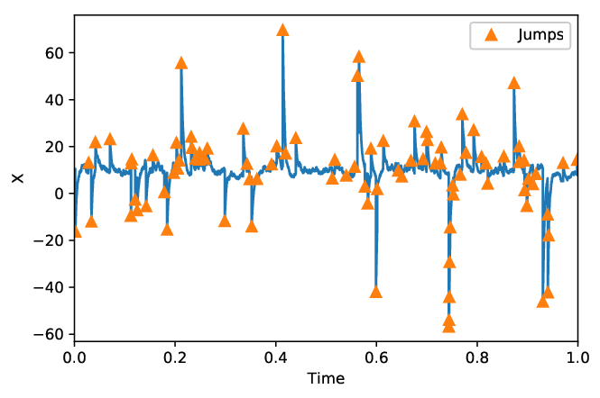
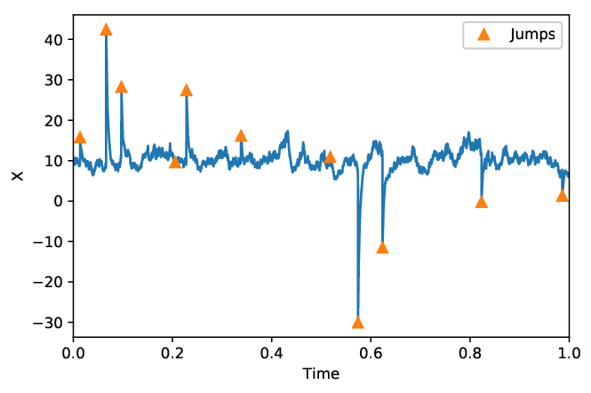
for some λ>0\lambda>0 and a probability measure ν⁡(d​x)\nu(dx) on ℝ{\mathbb{R}}. We thus model the electricity spot price as a classical continuous Itô semimartingale (Xtc)t≥0(X_{t}^{c})_{t\geq 0} allowing for the usual financial fluctuations and usual models (factor models, mean-reverting models and so on) to which we add a perturbation (Ztβ)t≥0(Z^{\beta}_{t})_{t\geq 0} of “spikes” or “jumps”, triggered by exogenous physical hazard, at intensity λ\lambda and magnitude ν⁡(d​x)\nu(dx), but with a relaxation period 1/β1/\beta comparable to λ\lambda that accounts for the absorption of such events by the market toward resulting in stable prices at large scales. The term comparable is a bit vague at this stage, and will be assessed precisely in Section 2.1, enabling us to speak of fast mean-reversion. In this setting, model (2)-(3)-(4) is well posed and can reproduce, at least visually, the general shape of electricity spot markets, compare historical data from Figure 1 and sample paths simulations given in Figure 2 and detailed in the simulation Section 3.2.
Refer to caption
(a) λn=10\lambda_{n}=10, βn=300\beta_{n}=300.
Refer to caption
(b) λn=10\lambda_{n}=10, βn=1000\beta_{n}=1000.
Refer to caption
(c) λn=75\lambda_{n}=75, βn=300\beta_{n}=300.
Figure 2. Simulation of the process XX in the case of a model having continuous part defined in (12) and with jump sizes having law 0.4​(−ℰ​(40))+0.6​ℰ​(30)0.4\left(-\mathcal{E}\left(40\right)\right)+0.6\mathcal{E}\left(30\right) for different values of λn\lambda_{n} and βn\beta_{n}.

Statistical setting

We assume that we observe the process (Xt)t≥0(X_{t})_{t\geq 0} given by (2)-(3)-(4) over the time interval [0,T][0,T] on a regular grid

0=t0,n<t1,n<…,tn,n=T,ti,n=i​Δn,for​  0≤i≤n,0=t_{0,n}<t_{1,n}<\ldots,t_{n,n}=T,\;t_{i,n}=i\Delta_{n},\;\;\text{for}\;\;0\leq i\leq n,

with mesh Δn\Delta_{n}. Thus we have nn (or rather n+1n+1) observations

(5) Xn=(X0,XΔn,…,Xn​Δn=XT).X^{n}=(X_{0},X_{\Delta_{n}},\ldots,X_{n\Delta_{n}}=X_{T}).

In the following, for a given process YY, we use the classical notations Δin​Y=Yti,n−Yti−1,n\Delta_{i}^{n}Y=Y_{t_{i,n}}-Y_{t_{i-1,n}} and Δ​Ys=Ys−Ys−\Delta Y_{s}=Y_{s}-Y_{s^{-}}.
Asymptotics are taken as n→∞n\rightarrow\infty. We assume that TT is constant, and we take T=1T=1 with no loss of generality. Equivalently, Δn=1/n→0\Delta_{n}=1/n\rightarrow 0 as n→∞n\rightarrow\infty. This asymptotic setting is usually referred to as the “high-frequency” framework (for instance the classical textbook [3] by Aït-Sahalia and Jacod), but this terminology is a bit misleading: our framework certainly belongs to statistical finance, but it has no link to high-frequency finance or microstructure modelling of any sort. In practice, we apply our methodology to three markets: the French EPEX, the German EPEX and the Australian electricity spot in Queensland, see Section 3 below. We use data between 2015, Jan. 01 and 2016, Dec. 31. with hourly data (even less in the case of Australian data), so that n=17064n=17064 is considered to be large. Equivalently, one hour is considered to be small in front of 2 years. In our setting, the important fact about the assumption that TT is fixed is that we leave out any stationarity or ergodicity of the underlying process. We thus make an implicit statistical robustness assumption, which we believe is of importance when considering recent and changing energy markets over such time horizons.

The parameters of interest are λ,β>0\lambda,\beta>0 that govern our correction formulas (see the application to forward contracts prices f⁡(t,T)f(t,T) below). In particular we leave out the issue of identifying the continuous semimartingale part (Xtc)t≥0(X_{t}^{c})_{t\geq 0} i.e. the drift (μt)t≥0(\mu_{t})_{t\geq 0} and the volatility process (σt)t≥0(\sigma_{t})_{t\geq 0} as well as the jump distribution ν⁡(d​x)\nu(dx) (only an estimation for the moments of ν\nu is proposed).

The mean-reversion factor over the observation increment [ti−1,n,ti,n][t_{i-1,n},t_{i,n}] is of size β​Δn\beta\Delta_{n}, and by requiring β​Δn\beta\Delta_{n} to be large compared to the order of magnitude Δn\sqrt{\Delta_{n}} of Δin​Xc\Delta_{i}^{n}X^{c} , we may hope to recover β\beta asymptotically. We thus introduce the asymptotic setting β=βn\beta=\beta_{n} with the requirement

(6) β=βn→∞​while​βn​Δn→∞.\beta=\beta_{n}\rightarrow\infty\;\;\text{while}\;\;\beta_{n}\sqrt{\Delta_{n}}\rightarrow\infty.

Condition (6) becomes

(7) βn​Δn​λn→∞\beta_{n}\sqrt{\Delta_{n}\lambda_{n}}\rightarrow\infty

if we let λ=λn→∞\lambda=\lambda_{n}\rightarrow\infty. A second crucial assumption is

(8) βn​Δn≲1,\beta_{n}\Delta_{n}\lesssim 1,

since otherwise, the spikes caused by the jumps of p¯\underline{p} are absorbed by the Brownian fluctuations of XcX^{c} due to the fast relaxation period 1/βn1/\beta_{n} and therefore cannot be detected by XnX^{n}.

Statistical results

Heavily relying on classical techniques in high-frequency finance (for instance [3, Theorem 10.26, p.374]), we estimate in a first step the times and sizes of the jumps which are random quantities, taking into account the interplay between βn\beta_{n}, λn\lambda_{n} and Δn\Delta_{n} dictated by the asymptotic regime (6)-(7)-(8), see Proposition 5. In a second step, we construct an estimator of βn\beta_{n} based on an estimator s^n\widehat{s}_{n} of the right-derivative or instantaneous slope of t↦Ztβt\mapsto Z^{\beta}_{t} right after a jump is detected. The estimator s^n\widehat{s}_{n} is based on averaging of instantaneous slope proxies of the form Δ​XTq​(1−e−βn​Δn)\Delta X_{T_{q}}(1-e^{-\beta_{n}\Delta_{n}}) that govern the relaxation effect after a jump of size Δ​XTq\Delta X_{T_{q}} has occurred at time TqT_{q} and it enables us to consider

β^n=−1Δn​log⁡(1−s^n)\widehat{\beta}_{n}=-\frac{1}{\Delta_{n}}\log\left(1-\widehat{s}_{n}\right)

as our estimator of βn\beta_{n}. Since βn\beta_{n} itself varies with nn and grows to infinity, the notion of convergence has to be considered carefully. Under suitable assumptions, we prove in Theorem 11 that the relative error

(9) ℰn=β^n−βnβn→0\mathcal{E}_{n}=\frac{\widehat{\beta}_{n}-\beta_{n}}{\beta_{n}}\rightarrow 0

in probability as n→∞n\rightarrow\infty. The error ℰn\mathcal{E}_{n} has two components: a first term of order 1/(βn​λn​Δn)1/(\beta_{n}\sqrt{\lambda_{n}\Delta_{n}}) due to Brownian oscillations, and a second term of order min⁡{λn/βn,1/βn}+λn/βn\min\{\lambda_{n}/\beta_{n},1/\sqrt{\beta_{n}}\}+\sqrt{\lambda_{n}}/\beta_{n} that accounts for the effect of jumps that are still present in the price process despite the relaxation effect. When βn​Δn​λn→∞\beta_{n}\sqrt{\Delta_{n}\lambda_{n}}\rightarrow\infty and λn/βn≲1\lambda_{n}/\beta_{n}\lesssim 1, we have ℰn\mathcal{E}_{n} converges to 00. If we assume further βn/λn→0\sqrt{\beta_{n}}/\lambda_{n}\rightarrow 0, we obtain a central limit theorem for ℰn\mathcal{E}_{n} with a Gaussian limit and an explicit rate of convergence that depends on the interplay between λn,βn\lambda_{n},\beta_{n} and Δn\Delta_{n}. We have an analogous result (although less demanding) for the estimation of the jump intensity λn\lambda_{n} detailed in Proposition 6.

Application to pricing forward contracts

We show in Theorem 12 that in the model for the spot price (with X=SX=S) defined by (2)-(3)-(4), the price f⁡(t,T)f(t,T) of a forward contract is given by

f⁡(t,T)=fc​(t,T)+fβ​(t,T),f\left(t,T\right)=f^{c}\left(t,T\right)+f^{\beta}\left(t,T\right),

where

fc​(t,T)=𝔼⁡[XTc|ℱt]f^{c}\left(t,T\right)=\mathbb{E}\big[X^{c}_{T}\,|\,\mathcal{F}_{t}\big]

and

fβ​(t,T)=e−β⁡(T−t)​Ztβ+λβ​∫ℝx​ν​(𝑑x)​(1−e−β⁡(T−t)).f^{\beta}\left(t,T\right)=e^{-\beta\left(T-t\right)}Z_{t}^{\beta}+\frac{\lambda}{\beta}\int_{{\mathbb{R}}}x\nu(dx)\left(1-e^{-\beta\left(T-t\right)}\right).

The term fc​(t,T)f^{c}\left(t,T\right) corresponds to the price of the forward contract in a continuous case framework. The computation of this value has been extensively studied for different continuous models and it is known analytically for the most common models, see for instance [5, 6] among others. The term fβ​(t,T)f^{\beta}\left(t,T\right) is a correction that follows from our approach. It is of order λ/β\lambda/\beta and is usually small for the applications we have in mind, see the practical implementation Sections 3 and 4. On balance, the presence of spikes does not significantly impact the price of forward contracts to within these order of magnitudes. This is consistent with our data, for which spikes are not observed on forward prices. By neglecting the term fβ​(t,T)f^{\beta}\left(t,T\right), we can calibrate the process XtcX^{c}_{t} to the observed forward prices and the process ZtβZ^{\beta}_{t} to the observed spot prices with the estimation procedure proposed in this paper. The results are similar for the modelling of the logarithm of the spot price (i.e when X=log⁡(S)X=\log(S)) by (2)-(3)-(4), see Theorem 13. We implement the prices of the forward contracts and Call options from a model calibrated to historical data on electricity prices in Section 4 and we show the impact of the spike modelling on the valuation of a strip of options with payoff of the form ∑i=1I(Sti,n−K)+\sum_{i=1}^{I}\left(S_{t_{i,n}}-K\right)^{+} for different times ti,nt_{i,n}. As expected, the value of this option increases if we add significant large spikes. In particular, we show that some out-of-the-money options have a significant value if we incorporate spikes in our modelling, while having a value close to 00 otherwise.

1.3. Organisation of the paper

Section 2 develops a rigorous mathematical framework for the stochastic model (2)-(3)-(4) and gives the explicit construction of the estimators described in Section 1.2 above together with their asymptotic properties in Propositions 5, 6 and Theorem 11. Section 3 establishes the numerical feasibility and consistency of our statistical estimation results on simulated and real data, based over two years (2015 and 2016) of electricity spot prices in three different markets (French, German and Australian). Section 4 is devoted to the application of our model and statistical results to forward contracts. We establish in Theorem 12 a correction formula to get analytical forward prices and study the valuation of a strip of European Call options. The proofs are given in Section 5.

2. Statistical results

2.1. Model assumptions

We consider the process (Xt)t≥0(X_{t})_{t\geq 0} defined by (2)-(3)-(4) in Section 1.2. Following closely the standard notation of Aït-Sahalia and Jacod [3], if ν\nu is a positive measure and ff a ν\nu-integrable function, we write f⁡(x)⋆ν=∫ℝf⁡(x)​ν​(𝑑x)f\left(x\right)\star\nu=\int_{\mathbb{R}}f\left(x\right)\nu\left(dx\right). Remember also that we work over a finite time horizon T=1T=1.

Assumption 1.

We have 𝔼⁡[(Xtc)2]<∞\mathbb{E}[(X_{t}^{c})^{2}]<\infty for every t≥0t\geq 0. Moreover, t↦σtt\mapsto\sigma_{t} is continuous on [0,1][0,1] and for some deterministic σ¯,σ¯,c0>0\underline{\sigma},\bar{\sigma},c_{0}>0, we have 0<σ¯2≤inftσt2≤suptσt2≤σ¯20<\underline{\sigma}^{2}\leq\inf_{t}\sigma_{t}^{2}\leq\sup_{t}\sigma_{t}^{2}\leq\bar{\sigma}^{2}, supt|μt|≤c0\sup_{t}|\mu_{t}|\leq c_{0}, ν⁡({0})=0\nu(\{0\})=0 and |x|2⋆ν<∞|x|^{2}\star\nu<\infty.

Since our asymptotic results will be given in distribution (see Theorem 11 below), the conditions on the drift (μt)t≥0(\mu_{t})_{t\geq 0} and (σt)t≥0(\sigma_{t})_{t\geq 0} can substantially be weakened (in order to accommodate for instance diffusion coefficients of the form σt=Xtc​h​(Xtc)\sigma_{t}=X_{t}^{c}h(X_{t}^{c}) with a bounded hh or even locally integrable) by standard localisation procedures, see for instance [18, Section 4.4.1]. We observe (5) and asymptotics are taken as n→∞n\rightarrow\infty or equivalently Δn=n−1→0\Delta_{n}=n^{-1}\rightarrow 0. We consider different asymptotic regimes for λ=λn\lambda=\lambda_{n} and β=βn\beta=\beta_{n}, compare Equations (6)-(7)-(8) and the accompanying discussion in Section 1.2 above.

Assumption 2.

We have

lim infnλn>0,λn≲βn,βn​Δn≲1,and​λn​Δn→0.\liminf_{n}\lambda_{n}>0,\;\;\lambda_{n}\lesssim\beta_{n},\;\;\beta_{n}\Delta_{n}\lesssim 1,\;\;\text{and}\;\;\lambda_{n}\Delta_{n}\rightarrow 0.

The condition λn≲βn\lambda_{n}\lesssim\beta_{n} ensures the stability of XtX_{t} as n→∞n\rightarrow\infty since Var⁡(Xt)=Var⁡(Xtc)+Var⁡(Ztβn)=Var⁡(Xtc)+|x|2⋆ν​λn​t2​βn​(1−e−2​βn)→∞\mathrm{Var}(X_{t})=\mathrm{Var}\left(X_{t}^{c}\right)+\mathrm{Var}(Z_{t}^{\beta_{n}})=\mathrm{Var}\left(X_{t}^{c}\right)+|x|^{2}\star\nu\,\frac{\lambda_{n}t}{2\beta_{n}}\left(1-e^{-2\beta_{n}}\right)\rightarrow\infty if supnλn/βn=∞\sup_{n}\lambda_{n}/\beta_{n}=\infty. The condition βn​Δn≲1\beta_{n}\Delta_{n}\lesssim 1 is necessary to identify spikes (or jumps): otherwise, a spike that occurs in the interval ((i−1)​Δn,i​Δn]\left(\left(i-1\right)\Delta_{n},i\Delta_{n}\right] will be absorbed by the relaxation effect before we observe Xi​ΔnX_{i\Delta_{n}}. Finally, the condition λn​Δn→0\lambda_{n}\Delta_{n}\rightarrow 0 controls the no accumulation of jumps within the rate of observation.

In order to estimate the times and sizes of the jumps, we need the following:

Assumption 3.

We have either (I)(I) or (I​I)(II), where

  1. (I)

    For some ϖ∈(0,1/2)\varpi\in\left(0,1/2\right):

    (i)λn2Δn→0,(ii)λn𝟏{|x|>Δn1/2−ϖ/(βnΔn)}⋆ν→0,and(iii)λn𝟏{|x|<Δn1/2−ϖ}⋆ν→0.\mathrm{(i)}\;\lambda_{n}^{2}\Delta_{n}\rightarrow 0,\;\;\mathrm{(ii)}\;\lambda_{n}{\bf 1}_{\{|x|>\Delta_{n}^{1/2-\varpi}/(\beta_{n}\Delta_{n})\}}\star\nu\rightarrow 0,\;\;\text{and}\;\;\mathrm{(iii)}\;\lambda_{n}{\bf 1}_{\{|x|<\Delta_{n}^{1/2-\varpi}\}}\star\nu\rightarrow 0.
  2. (II)

    For some ϖ∈(0,1/2)\varpi\in\left(0,1/2\right) and a sequence of integers kn≥1k_{n}\geq 1:

    (i)λn2Δnkn2→0,(ii)λn𝟏{|x|>eβn​Δn​knΔn1/2−ϖ}⋆ν→0,(iii)λn𝟏{|x|<Δn1/2−ϖ}⋆ν→0\mathrm{(i)}\;\lambda_{n}^{2}\Delta_{n}k^{2}_{n}\rightarrow 0,\;\;\mathrm{(ii)}\;\;\lambda_{n}{\bf 1}_{\{|x|>e^{\beta_{n}\Delta_{n}k_{n}}\Delta_{n}^{1/2-\varpi}\}}\star\nu\rightarrow 0,\;\;\mathrm{(iii)}\;\lambda_{n}{\bf 1}_{\{|x|<\Delta_{n}^{1/2-\varpi}\}}\star\nu\rightarrow 0

    and (iv)​λn​e−(βn​Δn1−ϖ)2→0\mathrm{(iv)}\;\lambda_{n}e^{-(\beta_{n}\Delta_{n}^{1-\varpi})^{2}}\rightarrow 0.

Assumption 3 (I) implies βn​Δn=o⁡(1)\beta_{n}\Delta_{n}=o\left(1\right). Condition (i) ensures that the number of jumps in an interval of size Δn\Delta_{n} is essentially 11. In the case where βn\beta_{n} is bounded, (ii) is implied by (i) and we have the usual conditions for the detection of jumps (see Mancini [23]). Condition (ii) controls the size of the mean-reversion. Condition (iii) controls the size of the small jumps that cannot converge too fast to 0. If the jumps are bounded below by some constant as Mancini [23] the condition is automatically satisfied.

Assumption 3 (II) (iv) implies that βn​Δn1−ϖ→∞\beta_{n}\Delta_{n}^{1-\varpi}\rightarrow\infty and in particular βn​Δn1/2→∞\beta_{n}\Delta_{n}^{1/2}\rightarrow\infty, implying that the mean reversion of order βn​Δn\beta_{n}\Delta_{n} is stronger than the order of magnitude Δn1/2\Delta_{n}^{1/2} of Brownian increments. It also allows for the case βn​Δn≈1\beta_{n}\Delta_{n}\approx 1. In the setting of Assumption 3 (II), the mean reversion is more difficult to distinguish from the jumps and in the case βn​Δn≈1\beta_{n}\Delta_{n}\approx 1, the jumps and the drift have the same size and are not distinguishable from their size solely. Condition (i) states that there is at most one jump in an interval of size knk_{n} which is large enough for the spike to vanish. Assumption 3 (II) also implies that λn2/βn→0\lambda_{n}^{2}/\beta_{n}\rightarrow 0. Assumption 3 (II) allows for high values of βn\beta_{n} but the number of jumps needs then to be smaller than in case of Assumption 3 (I) compared to βn\beta_{n}.

2.2. Estimation of the jump times and λn\lambda_{n}

We first construct estimators of the sequence of the jumps and of their intensity λn\lambda_{n}. Assumption 3 is in force. Let

Nt=∑s≤t𝟏{ΔXs≠0},t≥0,N_{t}=\sum_{s\leq t}{\bf 1}_{\{\Delta X_{s}\neq 0\}},\;\;t\geq 0,

denote the number of jumps of (Xt)t≥0(X_{t})_{t\geq 0} up to time tt and let T1<T2<⋯<Tq<⋯T_{1}<T_{2}<\cdots<T_{q}<\cdots denote the random times at which jumps occur. By construction, the sizes of jumps (Δ​XTq)q≥1\left(\Delta X_{T_{q}}\right)_{q\geq 1} form a sequence of independent and identically distributed random variables independent of (Nt)t≥0(N_{t})_{t\geq 0}. Let i⁡(n,q)i(n,q) be the random integer such that

(i⁡(n,q)−1)​Δn<Tq≤i⁡(n,q)​Δn.\left(i\left(n,q\right)-1\right)\Delta_{n}<T_{q}\leq i\left(n,q\right)\Delta_{n}.

We introduce the increasing sequence

1≤ℐn​(1)<ℐn​(2)<…<ℐn​(nmax)≤n1\leq\mathcal{I}_{n}\left(1\right)<\mathcal{I}_{n}(2)<\ldots<\mathcal{I}_{n}\big(n_{\max}\big)\leq n

of indices i∈{1,…,n}i\in\{1,\ldots,n\} defined by the realisation of the following successive events:

{|Δin​X|Δn>vn}under Assumption 3 (I)\Big\{\frac{|\Delta_{i}^{n}X|}{\sqrt{\Delta_{n}}}>v_{n}\Big\}\;\;\text{under Assumption \ref{assumpestimatorn}\, (I)}

and

{|Δin​X|Δn>vn,Δin​X​Δi+1n​X<0}​under Assumption 3 (II).\Big\{\frac{|\Delta_{i}^{n}X|}{\sqrt{\Delta_{n}}}>v_{n},\;\Delta_{i}^{n}X\Delta_{i+1}^{n}X<0\Big\}\;\;\text{under Assumption \ref{assumpestimatorn}\,(II)}.

with vn≍Δn−ϖv_{n}\asymp\Delta_{n}^{-\varpi}, following the notations of [3, Ch. 10]. The ℐn​(k)\mathcal{I}_{n}(k) define a subset of {1,…,n}\{1,\ldots,n\} that define in turn an estimator of λ\lambda via

λ^n=Card⁡{ℐn​(1),…,ℐn​(nmax)}=nmax.\widehat{\lambda}_{n}=\mathrm{Card}\big\{\mathcal{I}_{n}(1),\ldots,\mathcal{I}_{n}(n_{\max})\big\}=n_{\max}.

Under Assumption 3 (II), we need the supplementary condition Δin​X​Δi+1n​X<0\Delta_{i}^{n}X\Delta_{i+1}^{n}X<0 for the following reason: whenever a jump occurs, the mean reverting is dominant in the next observation interval and has a direction opposite to the sign of the jump. Furthermore, it enables us to discard the increments caused by the mean reversion that are large enough to be detected as jumps. Indeed, if we detect a false jump due to the mean reversion effect, the next increments will follow the same dynamics and it will share the same sign with first increment. The property that no jump lies within the next observation interval is ensured by the existence of knk_{n} defined in Assumption 3 (II).

Remark 4.

Note that λ^n\widehat{\lambda}_{n} is actually defined with two different algorithms, whether Assumption 3 (I) or 3 (II) is taken under consideration. When stating the results, we refer to the same notation λ^n\widehat{\lambda}_{n} that actually corresponds to two algorithms, which we will refer to as Algorithm (I ) and Algorithm (II) in the proofs and when processing the data, under Assumption 3 (I) and 3 (II) respectively.

Let

Ωn={λ^n=N1,∀q∈{1,…,N1}:Tq∈(ℐn(q)Δn−Δn,ℐn(q)Δn]}.\Omega_{n}=\Big\{\widehat{\lambda}_{n}=N_{1},\forall q\in\{1,...,N_{1}\}:T_{q}\in\big(\mathcal{I}_{n}(q)\Delta_{n}-\Delta_{n},\mathcal{I}_{n}(q)\Delta_{n}\big]\Big\}.
Proposition 5.

Work under Assumptions 1, 2 and 3. We have ℙ⁡(Ωn)→1\mathbb{P}\left(\Omega_{n}\right)\rightarrow 1.

The proof of Proposition 5 relies on a result of Aït-Sahalia and Jacod [3, Theorem 10.26, p.374]. However, the presence of a drift term −βn∫0tZsβnds-\beta_{n}\int_{0}^{t}Z_{s}^{\beta_{n}}ds that depends on nn together with the fact that λn→∞\lambda_{n}\rightarrow\infty makes the extension not trivial. Proposition 5 also provides us with an estimator λ^n\widehat{\lambda}_{n} of λn\lambda_{n}. In the case λn→∞\lambda_{n}\rightarrow\infty, we have the following asymptotic property:

Proposition 6.

Work under Assumption 1, 2 and 3 and assume that λn→∞\lambda_{n}\rightarrow\infty. We have

(10) λn​λ^n−λnλn→𝒩⁡(0,1)\sqrt{\lambda_{n}}\frac{\widehat{\lambda}_{n}-\lambda_{n}}{\lambda_{n}}\rightarrow\mathcal{N}(0,1)

in distribution as λn→∞\lambda_{n}\rightarrow\infty.

This result is straightforward: on the event Ωn\Omega_{n}, we have λ^n=N1\widehat{\lambda}_{n}=N_{1}, i.e. λ^n\widehat{\lambda}_{n} is a Poisson random variable with parameter λn\lambda_{n}, for which (10) holds. We conclude thanks to ℙ⁡(Ωn)→1\mathbb{P}\left(\Omega_{n}\right)\rightarrow 1.

Remark 7.

As for the optimality of the result, consider indeed the seemingly richer experiment where one continuously observes a Poisson process (𝒫t)0≤t≤1(\mathcal{P}_{t})_{0\leq t\leq 1} with intensity λ>0\lambda>0. The variable 𝒫1\mathcal{P}_{1} is a sufficient statistic and the Cramer-Rao bound tells us that any unbiased estimator λ^\widehat{\lambda} necessarily satisfies 𝔼⁡[(λ^−λ)2]≥I​(λ)−1\mathbb{E}[(\widehat{\lambda}-\lambda)^{2}]\geq I(\lambda)^{-1}, where I⁡(λ)=1+λ−1I(\lambda)=1+\lambda^{-1} is the Fisher information associated to the observation of 𝒫1\mathcal{P}_{1}, i.e. a Poisson random variable with parameter λ\lambda. Equivalently 𝔼⁡[(λ^−λλ)2]≥(λ−1+λ−2)∼λ−1\mathbb{E}\big[\big(\frac{\widehat{\lambda}-\lambda}{\lambda}\big)^{2}\big]\geq(\lambda^{-1}+\lambda^{-2})\sim\lambda^{-1} as λ→∞\lambda\rightarrow\infty which is consistent with the convergence (10) for fixed λ\lambda.

Remark 8.

The assumption λ→∞\lambda\rightarrow\infty may be acceptable for some electricity markets revealing a lot of extreme events, like for example in Australia. However, it can be questionable for electricity markets like in France or Germany, although the latter is currently revealing a lot of negative prices.

A natural estimator of the jump sizes is Δℐn​(q)n​X\Delta^{n}_{\mathcal{I}_{n}\left(q\right)}X for q∈{1,…,λ^n}q\in\{1,...,\widehat{\lambda}_{n}\}, see [3, Theorem 10.21, p.370]. In our case, Δℐn​(q)n​X\Delta^{n}_{\mathcal{I}_{n}\left(q\right)}X is equal to Δ​XTq​e−βn​(Tq−ℐn​(q)​Δn)\Delta X_{T_{q}}e^{-\beta_{n}\left(T_{q}-\mathcal{I}_{n}\left(q\right)\Delta_{n}\right)} plus a negligible term. If βn​Δn→0\beta_{n}\Delta_{n}\to 0, Δℐn​(q)n​X\Delta^{n}_{\mathcal{I}_{n}\left(q\right)}X is then equivalent to Δ​XTq\Delta X_{T_{q}} but if βn​Δn≍1\beta_{n}\Delta_{n}\asymp 1, the bias Δ​XTq​(1−e−βn​(Tq−ℐn​(q)​Δn))\Delta X_{T_{q}}\left(1-e^{-\beta_{n}\left(T_{q}-\mathcal{I}_{n}\left(q\right)\Delta_{n}\right)}\right) remains and it is not possible to identify the size of the jump. However, if λn→∞\lambda_{n}\to\infty, one can infer some statistical properties of the jumps size. We have the following result:

Proposition 9.

Work under Assumption 1, 2, 3 and assume that λn→∞\lambda_{n}\rightarrow\infty. Let m≥1∈ℕm\geq 1\in\mathbb{N} such that |x|2​m⋆ν<∞|x|^{2m}\star\nu<\infty,

m​βn​Δn(1−e−m​βn​Δn)​λ^n​∑q=1λ^n(Δℐn​(q)​X)m→xm⋆ν\frac{m\beta_{n}\Delta_{n}}{\left(1-e^{-m\beta_{n}\Delta_{n}}\right)\widehat{\lambda}_{n}}\sum_{q=1}^{\widehat{\lambda}_{n}}\left(\Delta_{\mathcal{I}_{n}\left(q\right)}X\right)^{m}\rightarrow x^{m}\star\nu

in probability as λn→∞\lambda_{n}\rightarrow\infty. Furthermore, if |x|3​m⋆ν<∞|x|^{3m}\star\nu<\infty,

λn​m​βn​Δn​(1−e−2​m​βn​Δn)2​(1−e−m​βn​Δn)2​(m​βn​Δn(1−e−m​βn​Δn)​λ^n​∑q=1λ^n(Δℐn​(q)​X)m−xm⋆ν)→𝒩⁡(0,1)\frac{\sqrt{\lambda_{n}}m\beta_{n}\Delta_{n}\left(1-e^{-2m\beta_{n}\Delta_{n}}\right)}{2(1-e^{-m\beta_{n}\Delta_{n}})^{2}}\left(\frac{m\beta_{n}\Delta_{n}}{\left(1-e^{-m\beta_{n}\Delta_{n}}\right)\widehat{\lambda}_{n}}\sum_{q=1}^{\widehat{\lambda}_{n}}\left(\Delta_{\mathcal{I}_{n}\left(q\right)}X\right)^{m}-x^{m}\star\nu\right)\rightarrow\mathcal{N}(0,1)

in distribution as λn→∞\lambda_{n}\rightarrow\infty.

Proof of Proposition 9 is immediate: it only requires the computation of ∫01e−βn​(t−⌊tΔn⌋​ΔnCLOSE​𝑑t=1−e−βn​Δnβn​Δn\int_{0}^{1}e^{-\beta_{n}(t-\lfloor\frac{t}{\Delta_{n}}\rfloor\Delta_{n}}dt=\frac{1-e^{-\beta_{n}\Delta_{n}}}{\beta_{n}\Delta_{n}} and the use of [28, Theorem 3] for the central limit theorem. Also, the proof for the case m=1m=1 appears in the proof of Theorem 11. We then omit the proof. Combining this result with our estimator of βn\beta_{n} provided below enables us to have an estimator for the moments of ν\nu.

2.3. Estimation of βn\beta_{n}

We are ready to construct an estimator of βn\beta_{n}, based on the estimation of the right-derivative or instantaneous slope of t↦Ztβt\mapsto Z^{\beta}_{t} right after a jump is detected. The estimator of this right-derivative, say sns_{n}, is based on averaging of instantaneous slope proxies of the form Δ​XTq​(1−e−βn​Δn)\Delta X_{T_{q}}(1-e^{-\beta_{n}\Delta_{n}}) that govern the relaxation effect after a jump of size Δ​XTq\Delta X_{T_{q}} has occurred at time TqT_{q} and it enables us to consider β^n=−1Δn​log⁡(1−s^n)\widehat{\beta}_{n}=-\frac{1}{\Delta_{n}}\log\left(1-\widehat{s}_{n}\right) as our estimator of βn\beta_{n}.

More precisely, let sgn⁡(x)=1\mathrm{\mathrm{sgn}}(x)=1 if x≥0x\geq 0 and −1-1 otherwise. On the event {λ^n>0}\{\widehat{\lambda}_{n}>0\}, define β^n\widehat{\beta}_{n} via

(11) exp⁡(−Δn​β^n)=max⁡{1+∑q=1λ^nsgn⁡(Δℐn​(q)n​X)​(Δℐn​(q)+1n​X+2​Δn​∑j=1q−1Δℐn​(j)n​X)∑q=1λ^n|Δℐn​(q)n​X|,Δn}\exp(-\Delta_{n}\widehat{\beta}_{n})=\max\Big\{1+\frac{\sum_{q=1}^{\widehat{\lambda}_{n}}\mathrm{\mathrm{sgn}}(\Delta^{n}_{\mathcal{I}_{n}(q)}X)\big(\Delta^{n}_{\mathcal{I}_{n}(q)+1}X+2\Delta_{n}\sum_{j=1}^{q-1}\Delta^{n}_{\mathcal{I}_{n}(j)}X\big)}{\sum_{q=1}^{\widehat{\lambda}_{n}}|\Delta^{n}_{\mathcal{I}_{n}(q)}X|},\Delta_{n}\Big\}

and set β^n=0\widehat{\beta}_{n}=0 otherwise. Our main result describes precisely the behaviour of β^n\widehat{\beta}_{n} under the different asymptotic regimes of interest.

Remark 10.

The same comments for β^n\widehat{\beta}_{n} as in Remark 4 for λ^n\widehat{\lambda}_{n} hold here.

Theorem 11.

Work under Assumptions 1, 2 and 3. Let βn​λn​Δn→∞\beta_{n}\sqrt{\lambda_{n}\Delta_{n}}\rightarrow\infty. On the set {λ^n>0}\{\widehat{\lambda}_{n}>0\}, we have

|β^n−βn|βn≲λn​Δn+1βn​λn​Δn+min⁡{1βn,λnβn}\frac{\big|\widehat{\beta}_{n}-\beta_{n}\big|}{\beta_{n}}\lesssim\lambda_{n}\Delta_{n}+\frac{1}{\beta_{n}\sqrt{\lambda_{n}\Delta_{n}}}+\min\left\{\frac{1}{\sqrt{\beta_{n}}},\frac{\lambda_{n}}{\beta_{n}}\right\}

in probability. More precisely,

  1. i)

    On {λ^n>0}\{\widehat{\lambda}_{n}>0\}, we have

    β^n−βnβn=ℳn+𝒱n​𝒥nT,\frac{\widehat{\beta}_{n}-\beta_{n}}{\beta_{n}}=\mathcal{M}_{n}+\mathcal{V}_{n}\mathcal{J}_{n}^{T},

    where

    ℳn=eβn​Δn​λnβn​(x⋆ν)​(sgn​(x)⋆ν)|x|⋆ν​(eβn​Δn−1βn​Δn−1),\mathcal{M}_{n}=e^{\beta_{n}\Delta_{n}}\frac{\lambda_{n}}{\beta_{n}}\frac{(x\star\nu)\;(\mathrm{\mathrm{sgn}}(x)\star\nu)}{|x|\star\nu}\big(\frac{e^{\beta_{n}\Delta_{n}}-1}{\beta_{n}\Delta_{n}}-1\big),

    𝒱n=(𝒱n(i))1≤i≤4∈ℝ4\mathcal{V}_{n}=(\mathcal{V}_{n}^{(i)})_{1\leq i\leq 4}\in{\mathbb{R}}^{4} is such that

    {𝒱n(1)=eβn​Δn​λn3​βn​|x|⋆ν​((sgn⁡(x)⋆ν)2​(|x|2⋆ν)+(x⋆ν)2−2​(sgn⁡(x)⋆ν)​(|x|2⋆ν))1/2,𝒱n(2)=eβn​Δn​min⁡{(|x|2⋆ν(|x|⋆ν)2​12​βn​(1−e−2​βn​Δn)2​βn​Δn)1/2,λnβn},𝒱n(3)=eβn​Δn​(βn​Δn1−e−βn​Δn)​∫01σs2​𝑑s|x|⋆ν​λn​βn​Δn,𝒱n(4)=eβn​Δn​∫01σs2​𝑑s​Δn|x|⋆ν​λn,\left\{\begin{array}[]{ll}\mathcal{V}_{n}^{(1)}&=e^{\beta_{n}\Delta_{n}}\frac{\sqrt{\lambda_{n}}}{\sqrt{3}\beta_{n}|x|\star\nu}\big((\mathrm{\mathrm{sgn}}(x)\star\nu)^{2}(|x|^{2}\star\nu)+(x\star\nu)^{2}-2(\mathrm{\mathrm{sgn}}(x)\star\nu)(|x|^{2}\star\nu)\big)^{1/2},\\ \\ \mathcal{V}_{n}^{(2)}&=e^{\beta_{n}\Delta_{n}}\min\big\{\big(\tfrac{|x|^{2}\star\nu}{(|x|\star\nu)^{2}}\frac{1}{2\beta_{n}}\frac{(1-e^{-2\beta_{n}\Delta_{n}})}{2\beta_{n}\Delta_{n}}\big)^{1/2},\frac{\lambda_{n}}{\beta_{n}}\big\},\\ \\ \mathcal{V}_{n}^{(3)}&=e^{\beta_{n}\Delta_{n}}\big(\frac{\beta_{n}\Delta_{n}}{1-e^{-\beta_{n}\Delta_{n}}}\big)\frac{\sqrt{\int_{0}^{1}\sigma_{s}^{2}ds}}{|x|\star\nu\sqrt{\lambda_{n}}\beta_{n}\sqrt{\Delta_{n}}},\\ \\ \mathcal{V}_{n}^{(4)}&=e^{\beta_{n}\Delta_{n}}\frac{\sqrt{\int_{0}^{1}\sigma_{s}^{2}ds}\sqrt{\Delta_{n}}}{|x|\star\nu\sqrt{\lambda_{n}}},\end{array}\right.

    and 𝒥n=(𝒥n(i))1≤i≤4∈ℝ4\mathcal{J}_{n}=(\mathcal{J}_{n}^{(i)})_{1\leq i\leq 4}\in{\mathbb{R}}^{4} is bounded in probability as n→∞n\rightarrow\infty.

  2. ii)

    If λn→∞\lambda_{n}\rightarrow\infty, then

    (𝒥n(3),𝒥n(4))→𝒩⁡(0,Idℝ2)(\mathcal{J}_{n}^{(3)},\mathcal{J}_{n}^{(4)})\rightarrow\mathcal{N}(0,\mathrm{Id}_{{\mathbb{R}}^{2}})

    in distribution as n→∞n\rightarrow\infty.

  3. iii)

    If λn→∞\lambda_{n}\rightarrow\infty, |x|3⋆ν<∞|x|^{3}\star\nu<\infty and (sgn⁡(x)⋆ν)2​|x|2⋆ν+(x⋆ν)2−2​sgn​(x)⋆ν​|x|2⋆ν≠0,(\mathrm{\mathrm{sgn}}(x)\star\nu)^{2}|x|^{2}\star\nu+(x\star\nu)^{2}-2\mathrm{\mathrm{sgn}}(x)\star\nu|x|^{2}\star\nu\neq 0, we have

    (𝒥n(1),𝒥n(3),𝒥n(4))→𝒩⁡(0,Idℝ3)(\mathcal{J}_{n}^{(1)},\mathcal{J}_{n}^{(3)},\mathcal{J}_{n}^{(4)})\rightarrow\mathcal{N}(0,\mathrm{Id}_{{\mathbb{R}}^{3}})

    in distribution as n→∞n\rightarrow\infty.

  4. iv)

    If βn/λn2→0\beta_{n}/\lambda_{n}^{2}\rightarrow 0, the conditions of OPENiii)\mathrm{iii)} and |x|4⋆ν<∞|x|^{4}\star\nu<\infty hold together, we finally obtain

    𝒥n→𝒩⁡(0,Idℝ4)\mathcal{J}_{n}\rightarrow\mathcal{N}(0,\mathrm{Id}_{{\mathbb{R}}^{4}})

    in distribution as n→∞n\rightarrow\infty.

Some remarks on the different error terms: 1) the term of order 1/(βn​λn​Δn)1/(\beta_{n}\sqrt{\lambda_{n}\Delta_{n}}) accounts for the presence of a Brownian motion in the term (Xtc)t≥0(X^{c}_{t})_{t\geq 0}. When λn\lambda_{n} is bounded, we need βn​Δn→∞\beta_{n}\sqrt{\Delta_{n}}\rightarrow\infty or equivalently Δn=o⁡(βn​Δn)\sqrt{\Delta_{n}}=o\left(\beta_{n}\Delta_{n}\right): the size of the slope of (Ztβ)t≥0(Z^{\beta}_{t})_{t\geq 0} after a jump needs to dominate the Brownian motion part which is of order Δn\sqrt{\Delta_{n}}. In the case where λn→∞\lambda_{n}\rightarrow\infty, we can average the error due to the Brownian martingale part and then diminish the order of the error. In that case, we do not need the restriction Δn=o⁡(βn​Δn)\sqrt{\Delta_{n}}=o\left(\beta_{n}\Delta_{n}\right) anymore but rather Δn/λn=o⁡(βn​Δn)\sqrt{\Delta_{n}/\lambda_{n}}=o\left(\beta_{n}\Delta_{n}\right). 2) The error terms of order min⁡{1βn,λnβn}\min\{\frac{1}{\sqrt{\beta_{n}}},\frac{\lambda_{n}}{\beta_{n}}\}, λnβn\frac{\sqrt{\lambda_{n}}}{\beta_{n}} and λn​Δn\lambda_{n}\Delta_{n} account for the jumps that occur before the observation increment used to estimate the slope of the process. 3) The term 2​Δn​∑j=1q−1Δℐn​(j)n​X2\Delta_{n}\sum_{j=1}^{q-1}\Delta^{n}_{\mathcal{I}_{n}(j)}X introduced in the definition of β^n\widehat{\beta}_{n} in (11) is a bias correction that enables us to obtain a consistent estimator in the case λn/βn≈1\lambda_{n}/\beta_{n}\approx 1.

3. Practical implementation

3.1. Choice of the threshold vnv_{n}

The method to detect the jumps is based on the classical use of the threshold which is proportional to Δn−ϖ\Delta_{n}^{-\varpi}. As for the choice of the threshold and ϖ\varpi, no exact method is provided in the literature. However, the threshold is recommended to be chosen of the form vn=C​σ^​Δn−ϖv_{n}=C\hat{\sigma}\Delta_{n}^{-\varpi} in [2, Section 5.3] and [3, Section 6.2.2, p. 187] where CC is a constant and σ^\hat{\sigma} is an estimator of the integrated volatility, defined by (∫01σs2​𝑑s)1/2(\int_{0}^{1}\sigma_{s}^{2}ds)^{1/2} (actually, the square root of the integrated square volatility). A popular rule-of-thumb consists in picking ϖ\varpi close to 00. Moreover, [2] suggests to choose CC between 3 and 5.

It remains to find an estimator of the integrated volatility (∫01σs2​𝑑s)1/2(\int_{0}^{1}\sigma_{s}^{2}ds)^{1/2}. A natural choice is the multipower variation estimator defined by

σ^=(Γ⁡(12)21k​Γ​(12+1k))k​∑i=1n−k|Δin​X​Δi+1n​X​…​Δi+kn​X|2k\hat{\sigma}=\sqrt{\Big(\frac{\Gamma(\frac{1}{2})}{2^{\frac{1}{k}}\Gamma(\frac{1}{2}+\frac{1}{k})}\Big)^{k}\sum_{i=1}^{n-k}|\Delta_{i}^{n}X\Delta_{i+1}^{n}X\ldots\Delta_{i+k}^{n}X|^{\frac{2}{k}}}

with kk the order of the estimator, see [4] and [33] for more details. The order of the multipower variation estimator is set to 20 in the practical applications in this paper, which is high compared to the orders typically chosen in the literature. This choice is justified by the strong mean reversion of the spikes. As for the jumps, spikes have large increments that need to be compensated in the multipower variation estimator and can be present during two or three time steps. We compensate these large increments with a higher order of the multipower variation. Some simulations on simple models show that an order of 20 looks reasonable.

3.2. Numerical illustration

In this section, we study the performances of our estimation procedures on simulated data of the process defined by (2)-(3)-(4). We tested a wide range of values for (λn,βn)(\lambda_{n},\beta_{n}) in order to illustrate the results of Theorem 11. To be consistent with real data, the process is simulated with a step time Δn=10−4\Delta_{n}=10^{-4}, which is the order of magnitude corresponding to one year of hourly data observations. We pick

(12) d​Xtc=Xtc​((2−100​log⁡(Xtc))​d​t+2​d​Wt)dX^{c}_{t}=X^{c}_{t}\big((2-100\log(X^{c}_{t}))dt+2dW_{t}\big)

corresponding to the exponential of an Ornstein-Uhlenbeck process with the mean reverting parameter equal to 100 and volatility parameter equal to 2. The sizes of the jumps follow the law 0.4​(−ℰ​(15))+0.6​ℰ​(10)0.4\left(-\mathcal{E}\left(15\right)\right)+0.6\mathcal{E}\left(10\right), with ℰ⁡(ρ)\mathcal{E}(\rho) denoting the exponential distribution with parameter ρ>0\rho>0. Figure 2 illustrates a sample path of the process for different parameters λn\lambda_{n} and βn\beta_{n}. We realize 10000 simulations. We use jump detection using Algorithm (I), corresponding only to the use of a threshold, as well as Algorithm (II), corresponding to filtering the previous jumps by keeping only increments that have successive opposite signs, respectively working theoretically in the case of 3 (I) and 3 (II).

Table 1, 2 and 3 show the different results of estimated (λ^n,β^n)(\widehat{\lambda}_{n},\widehat{\beta}_{n}) using a threshold equal to C​σ^​Δn−0.01C\hat{\sigma}\Delta_{n}^{-0.01}, for C=3, 4, 5C=3,\;4,\;5. As expected, for large βn\beta_{n}, the estimation on filtered jumps gives satisfactory results of β^n\widehat{\beta}_{n}, whatever the value of λn\lambda_{n} satisfying the different assumptions, and seems to slightly underestimate λn\lambda_{n}, whereas the estimation under Algorithm (I) gives bad results on β^n\widehat{\beta}_{n} and overestimates λn\lambda_{n}.

The results for βn=20\beta_{n}=20 highlights, as expected, the need in Assumption 3 (II) to have a small number of jumps (λn=10\lambda_{n}=10) to get satisfactory results. Because of the expected βn\beta_{n} on real data, we will focus, in the next section, on the estimation procedure on filtered jumps (i.e. using Algorithm (II). This choice is also justified by the fact that underestimating the numbers of spikes seems to have a lower impact on the quality of β^n\widehat{\beta}_{n} than overestimating them. One also observes that the choice of CC has an impact on the estimation of λn\lambda_{n}: the threshold to select jumps increases with CC and then the estimated λn\lambda_{n} which is the number of jumps decreases. On the contrary, it has a low impact on the estimation of βn\beta_{n}, except in the case C=3C=3 for small λn\lambda_{n} where the number of spikes is overestimated, leading to a bad estimator for βn\beta_{n}. Finally, the impact of the order of the multipower estimator of the volatility is illustrated in Figure 3. The impact is negligible from an order of 2020, where the estimators mean of λn\lambda_{n} and βn\beta_{n} remain constant and give a good estimation. Before 20, it has only an impact on the estimation of λn\lambda_{n}: the spike effect has not disappeared in the estimator and σ^\hat{\sigma} is overestimated, inducing less detected spikes and an underestimation for λn\lambda_{n}. This supports the choice of a high order for the multipower estimator.

(λn,βn)\left(\lambda_{n},\beta_{n}\right) Algorithm (I) Algorithm (II)
λ^n\widehat{\lambda}_{n} β^n\widehat{\beta}_{n} λ^n\widehat{\lambda}_{n} β^n\widehat{\beta}_{n}
Mean C. I. Mean C. I. Mean C. I. Mean C. I.
(10,2)(10,2) 27.0 [18,36]\left[18,36\right] 4.4 [−16.6,25.8]\left[-16.6,25.8\right] 13.3 [8,20]\left[8,20\right] 86.5 [13.6,179.6]\left[13.6,179.6\right]
(10,20)(10,20) 21.3 [11,35]\left[11,35\right] -31.6 [−152.2,23.7]\left[-152.2,23.7\right] 8.9 [5,14]\left[5,14\right] 37.1 [18.1,66.8]\left[18.1,66.8\right]
(10,200)(10,200) 95.1 [70,117]\left[70,117\right] -592.6 [−1839.0,28.7]\left[-1839.0,28.7\right] 9.4 [5,15]\left[5,15\right] 204.5 [186.5,225.7]\left[186.5,225.7\right]
(10,2000)(10,2000) 94.1 [54,137]\left[54,137\right] -4430.1 [−5860.2,−2271.0]\left[-5860.2,-2271.0\right] 9.7 [5,15]\left[5,15\right] 2003.0 [1978.9,2026.2]\left[1978.9,2026.2\right]
(10,20000)(10,20000) 45.7 [31,62]\left[31,62\right] -727.9 [−1262.9,−77.7]\left[-1262.9,-77.7\right] 18.0 [12,25]\left[12,25\right] 19152.0 [17840.8,19845.5]\left[17840.8,19845.5\right]
(75,2)(75,2) 79.6 [66,94]\left[66,94\right] 2.2 [−2.3,6.6]\left[-2.3,6.6\right] 42.1 [32,53]\left[32,53\right] 42.5 [−3.5,232.1]\left[-3.5,232.1\right]
(75,20)(75,20) 73.0 [59,88]\left[59,88\right] 19.7 [12.4,27.8]\left[12.4,27.8\right] 49.5 [39,60]\left[39,60\right] 50.6 [24.4,158.9]\left[24.4,158.9\right]
(75,200)(75,200) 106.7 [82,132]\left[82,132\right] 147.0 [94.5,190.7]\left[94.5,190.7\right] 63.3 [52,75]\left[52,75\right] 226.2 [198.8,289.4]\left[198.8,289.4\right]
(75,2000)(75,2000) 351.3 [290,411]\left[290,411\right] -2483.0 [−3471.0,−1566.8]\left[-3471.0,-1566.8\right] 69.4 [56,83]\left[56,83\right] 2021.5 [1959.7,2116.0]\left[1959.7,2116.0\right]
(75,20000)(75,20000) 229.2 [189,271]\left[189,271\right] -1158.3 [−1291.5,−1016.8]\left[-1291.5,-1016.8\right] 80.4 [66,96]\left[66,96\right] 19717.3 [18745.8,20257.2]\left[18745.8,20257.2\right]
Table 1. Performance of (λ^n,β^n)(\widehat{\lambda}_{n},\widehat{\beta}_{n}) for different values of (λn,βn)\left(\lambda_{n},\beta_{n}\right) using Algorithms (I) and (II), with continuous part defined by (12) and jump size distribution 0.4​(−ℰ​(15))+0.6​ℰ​(10)0.4\left(-\mathcal{E}\left(15\right)\right)+0.6\mathcal{E}\left(10\right). The threshold vnv_{n} is chosen equal to 3​σ^​Δn−0.013\hat{\sigma}\Delta_{n}^{-0.01} with σ^\hat{\sigma} is the multi-power variation estimator of order 20. The means and quantile intervals 5%-95% are computed with 10410^{4} Monte-Carlo simulations and Δn=10−4\Delta_{n}=10^{-4}.
(λn,βn)\left(\lambda_{n},\beta_{n}\right) Algorithm (I) Algorithm (II)
λ^n\widehat{\lambda}_{n} β^n\widehat{\beta}_{n} λ^n\widehat{\lambda}_{n} β^n\widehat{\beta}_{n}
Mean C. I. Mean C. I. Mean C. I. Mean C. I.
(10,2)(10,2) 10.6 [6,16]\left[6,16\right] 2.0 [−9.7,13.7]\left[-9.7,13.7\right] 5.8 [2,10]\left[2,10\right] 29.7 [4.6,46.4]\left[4.6,46.4\right]
(10,20)(10,20) 10.2 [5,16]\left[5,16\right] 18.4 [2.4,32.4]\left[2.4,32.4\right] 7.6 [4,12]\left[4,12\right] 29.0 [16.8,41.3]\left[16.8,41.3\right]
(10,200)(10,200) 54.8 [39,69]\left[39,69\right] -256.6 [−996.6,114.1]\left[-996.6,114.1\right] 9.3 [5,14]\left[5,14\right] 203.8 [186.5,224.9]\left[186.5,224.9\right]
(10,2000)(10,2000) 81.5 [47,118]\left[47,118\right] -4216.3 [−5908.7,−1902.0]\left[-5908.7,-1902.0\right] 9.6 [5,15]\left[5,15\right] 2002.8 [1978.9,2025.7]\left[1978.9,2025.7\right]
(10,20000)(10,20000) 30.9 [16,48]\left[16,48\right] -1151.6 [−1528.6,−742.1]\left[-1528.6,-742.1\right] 10.8 [5,17]\left[5,17\right] 19778.4 [19185.2,20168.1]\left[19185.2,20168.1\right]
(75,2)(75,2) 74.2 [61,89]\left[61,89\right] 2.0 [−2.4,6.2]\left[-2.4,6.2\right] 40.2 [30,51]\left[30,51\right] 40.5 [−3.8,221.3]\left[-3.8,221.3\right]
(75,20)(75,20) 72.3 [59,87]\left[59,87\right] 19.8 [12.8,27.8]\left[12.8,27.8\right] 49.2 [39,60]\left[39,60\right] 50.4 [24.4,158.9]\left[24.4,158.9\right]
(75,200)(75,200) 77.3 [61,97]\left[61,97\right] 178.8 [139.1,212.2]\left[139.1,212.2\right] 62.1 [51,74]\left[51,74\right] 225.4 [198.2,287.8]\left[198.2,287.8\right]
(75,2000)(75,2000) 281.7 [231,330]\left[231,330\right] -1888.3 [−2843.5,−1004.8]\left[-2843.5,-1004.8\right] 67.4 [55,81]\left[55,81\right] 2020.8 [1959.3,2114.6]\left[1959.3,2114.6\right]
(75,20000)(75,20000) 216.7 [177,257]\left[177,257\right] -1200.1 [−1307.8,−1085.3]\left[-1307.8,-1085.3\right] 76.6 [62,91]\left[62,91\right] 19760.4 [18778.1,20302.9]\left[18778.1,20302.9\right]
Table 2. Performance of (λ^n,β^n)(\widehat{\lambda}_{n},\widehat{\beta}_{n}) for different values of (λn,βn)\left(\lambda_{n},\beta_{n}\right) using Algorithmes (I) and (II), with continuous part defined by (12) and jump size distribution 0.4​(−ℰ​(15))+0.6​ℰ​(10)0.4\left(-\mathcal{E}\left(15\right)\right)+0.6\mathcal{E}\left(10\right). The threshold vnv_{n} is chosen equal to 4​σ^​Δn−0.014\hat{\sigma}\Delta_{n}^{-0.01} with σ^\hat{\sigma} is the multi-power variation estimator of order 20. The means and quantile intervals 5%-95% are computed with 10410^{4} Monte-Carlo simulations and Δn=10−4\Delta_{n}=10^{-4}.
(λn,βn)\left(\lambda_{n},\beta_{n}\right) Algorithm (I) Algorithm (II)
λ^n\widehat{\lambda}_{n} β^n\widehat{\beta}_{n} λ^n\widehat{\lambda}_{n} β^n\widehat{\beta}_{n}
Mean C. I. Mean C. I. Mean C. I. Mean C. I.
(10,2)(10,2) 9.959.95 [5,15]\left[5,15\right] 2.01 [−9.21,12.85]\left[-9.21,12.85\right] 5.455.45 [2,9]\left[2,9\right] 19.5 [4.26,39.4]\left[4.26,39.4\right]
(10,20)(10,20) 9.99.9 [5,15]\left[5,15\right] 19.84 [7.6,32.4]\left[7.6,32.4\right] 7.57.5 [3,12]\left[3,12\right] 28.8 [16.9,40.2]\left[16.9,40.2\right]
(10,200)(10,200) 33.433.4 [17,47]\left[17,47\right] -76.7 [−540,158]\left[-540,158\right] 9.39.3 [5,14]\left[5,14\right] 204 [188,224]\left[188,224\right]
(10,2000)(10,2000) 72.572.5 [42,105]\left[42,105\right] -3968 [−5934,−1633]\left[-5934,-1633\right] 9.69.6 [5,15]\left[5,15\right] 2002 [1979,2023]\left[1979,2023\right]
(10,20000)(10,20000) 29.229.2 [15,46]\left[15,46\right] -1207 [−1508,−871]\left[-1508,-871\right] 10.210.2 [5,16]\left[5,16\right] 19861 [19337,20207]\left[19337,20207\right]
(75,2)(75,2) 73.773.7 [60,88]\left[60,88\right] 2 [−2.46,6.17]\left[-2.46,6.17\right] 39.939.9 [30,51]\left[30,51\right] 39.2 [−4,204]\left[-4,204\right]
(75,20)(75,20) 71.971.9 [59,86]\left[59,86\right] 19.8 [12.9,27.6]\left[12.9,27.6\right] 49.949.9 [39,60]\left[39,60\right] 49.9 [24.5,155.6]\left[24.5,155.6\right]
(75,200)(75,200) 68.768.7 [55,83]\left[55,83\right] 191 [157,219]\left[157,219\right] 6161 [50,73]\left[50,73\right] 225 [198,291]\left[198,291\right]
(75,2000)(75,2000) 234234 [192,273]\left[192,273\right] -1403 [−2334,−556]\left[-2334,-556\right] 65.665.6 [54,78]\left[54,78\right] 2019 [1958,2109]\left[1958,2109\right]
(75,20000)(75,20000) 207207 [170,247]\left[170,247\right] -1216 [−1308,−1113]\left[-1308,-1113\right] 74.274.2 [60,89]\left[60,89\right] 19785 [18790,20310]\left[18790,20310\right]
Table 3. Performance of (λ^n,β^n)(\widehat{\lambda}_{n},\widehat{\beta}_{n}) for different values of (λn,βn)\left(\lambda_{n},\beta_{n}\right) using Algorithmes (I) and (II), with continuous part defined by (12) and jump size distribution 0.4​(−ℰ​(15))+0.6​ℰ​(10)0.4\left(-\mathcal{E}\left(15\right)\right)+0.6\mathcal{E}\left(10\right). The threshold vnv_{n} is chosen equal to 5​σ^​Δn−0.015\hat{\sigma}\Delta_{n}^{-0.01} with σ^\hat{\sigma} is the multi-power variation estimator of order 20. The means and quantile intervals 5%-95% are computed with 10410^{4} Monte-Carlo simulations and Δn=10−4\Delta_{n}=10^{-4}.
Refer to caption
(a) Estimation of λn\lambda_{n}.
Refer to caption
(b) Estimation of βn\beta_{n}.
Figure 3. Estimation of (λ^n,β^n)(\widehat{\lambda}_{n},\widehat{\beta}_{n}) for different values of the order of the multipower estimator of the volatility σ^\hat{\sigma} using Algorithm (II), with continuous part defined by (12), λn=75\lambda_{n}=75, βn=20000\beta_{n}=20000 and jump size distribution 0.4​(−ℰ​(15))+0.6​ℰ​(10)0.4\left(-\mathcal{E}\left(15\right)\right)+0.6\mathcal{E}\left(10\right). The threshold vnv_{n} is chosen equal to 5​σ^​Δn−0.015\hat{\sigma}\Delta_{n}^{-0.01}. The mean of the estimators is computed with 10410^{4} Monte-Carlo simulations and Δn=10−4\Delta_{n}=10^{-4}.

3.3. Practical implementation on real data

Electricity spot historical data do exhibit spikes with strong mean reversion, see Figure 1. We expect to obtain relatively high values for βn\beta_{n}, a necessary condition in order to apply our estimation procedure, especially under Assumption 3 (II). The goal is then to estimate the parameters λn\lambda_{n} and βn\beta_{n} of the process ZβnZ^{\beta_{n}} on a time series of spot prices, assuming that the spot price is the sum of a continuous semimartingale and a spike process. We dispose of the following data:

  1. (1)

    French electricity EPEX spot prices between the first of January of 2015 (included) and the first of January 2017 (not included) with data each hour 11 1 Source: https://www.epexspot.com/,

  2. (2)

    German electricity EPEX spot prices between the first of January of 2015 (included) and the first of January 2017 (not included) with data each hour 1,

  3. (3)

    Australian electricity spot prices in Queensland between the first of January of 2015 (included) and the first of January 2017 (not included) with data each 30 minutes 22 2 Source: https://www.aemo.com.au/.

We estimate those parameters using a threshold vn=C​σ^​Δn−0.01v_{n}=C\hat{\sigma}\Delta_{n}^{-0.01}, with σ^\hat{\sigma} the multi-power variation of order 20 and CC a constant set to 3, 4 or 5. Results are presented in Table 4. Equivalent half-life time in h​o​u​r​s−1hours^{-1}, log⁡(2)β^n​Δn\frac{\log(2)}{\hat{\beta}_{n}\Delta_{n}}, and intensity λ^n2\frac{\hat{\lambda}_{n}}{2} in years-1 are given Table 5. Figure 1 gives the time series of these three sets of data with jumps time estimated in the case C=5C=5.
As expected, the estimated λ^n\widehat{\lambda}_{n} is sensitive to the value of CC, the number of detected jumps decreasing with CC. The estimated β^n\widehat{\beta}_{n} is much less sensitive, although we can observe a slight increase of values with CC in the French and German markets. We will see in section 4.3 the sensitivity of these estimators to the value of a strip of Call options.

Market C=3C=3 C=4C=4 C=5C=5
French (100,19170)\left(100,19170\right) (51,20259)\left(51,20259\right) (35,21043)\left(35,21043\right)
German (145,9848)\left(145,9848\right) (62,13438)\left(62,13438\right) (34,14531)\left(34,14531\right)
Australian (337,22897)\left(337,22897\right) (227,22883)\left(227,22883\right) (177,22884)\left(177,22884\right)
Table 4. Estimation of (λn,βn)\left(\lambda_{n},\beta_{n}\right) for different markets using a threshold of the form vn=C​σ^​Δn−0.01v_{n}=C\hat{\sigma}\Delta_{n}^{-0.01} where σ^\hat{\sigma} is the multi-power variation estimator of order 20 and CC takes different values.
Market C=3C=3 C=4C=4 C=5C=5
French (50,0.63)\left(50,0.63\right) (25.5,0.60)\left(25.5,0.60\right) (17.5,0.58)\left(17.5,0.58\right)
German (72.5,1.23)\left(72.5,1.23\right) (31,0.90)\left(31,0.90\right) (17,0.83)\left(17,0.83\right)
Australian (168.5,1.06)\left(168.5,1.06\right) (113.5,1.06)\left(113.5,1.06\right) (88.5,1.06)\left(88.5,1.06\right)
Table 5. Estimation of intensity λ^n2\frac{\hat{\lambda}_{n}}{2} in years-1 (first component) and half-life time in h​o​u​r​s−1hours^{-1}, log⁡(2)β^n​Δn\frac{\log(2)}{\hat{\beta}_{n}\Delta_{n}} (second component), for different markets using a threshold of the form vn=C​σ^​Δn−0.01v_{n}=C\hat{\sigma}\Delta_{n}^{-0.01} where σ^\hat{\sigma} is the multi-power variation estimator of order 20 and CC takes different values.

In the previous analysis, one neglects the intraday seasonality which can be very strong and induce spikes detection, see Figure 4. Indeed, the spot price is not an hourly process but a daily process. Spot fixing is done every day and the 24 prices for next day are settled simultaneously. However, representing this 24-dimensional stochastic process is very difficult and more importantly not suitable for risk management. Table 6 contains the estimation results on the different data set with data sampled daily for each hour and for the daily average spot price using C=4C=4 for the threshold parameter (intensity λ^n2\frac{\hat{\lambda}_{n}}{2} in years-1 and half-life time in days-1, log⁡(2)β^n​Δn\frac{\log(2)}{\hat{\beta}_{n}\Delta_{n}}, are given). Our estimation procedure provides an estimation for jump times, jump sizes, and for the parameter β\beta. However, the number of identified spike being low, the estimation procedure can not provide a robust estimation of λ\lambda. Figure 5 represents the spike estimation for hours 0 and 18. Some spikes, for instance during January 2016 and hour 21, are not detected: they are not a spike in our modelling because for the spot to be high, several time steps are needed and it is not seen as a discontinuity.

Refer to caption
Figure 4. German hourly spot price between 2016-01-20 and 2016-01-25.
Country French German Australian
Hour / Parameters λ^n2\frac{\hat{\lambda}_{n}}{2} log⁡(2)β^n​Δn\frac{\log(2)}{\hat{\beta}_{n}\Delta_{n}} λ^n2\frac{\hat{\lambda}_{n}}{2} log⁡(2)β^n​Δn\frac{\log(2)}{\hat{\beta}_{n}\Delta_{n}} λ^n2\frac{\hat{\lambda}_{n}}{2} log⁡(2)β^n​Δn\frac{\log(2)}{\hat{\beta}_{n}\Delta_{n}}
Day 1.0 2.07 0.5 15.5 0.46
0 1.0 1.35 8.5 1.23 5.0 1.76
1 1.5 1.67 9.5 1.23 7.5 0.55
2 0.5 2.67 8.5 0.65 4.5 0.82
3 0.5 1.94 8.5 1.02 4.0 0.55
4 1.0 3.73 5.5 0.78 4.5 0.46
5 1.5 4.39 5.0 1.06 3.0 3.65
6 0.0 2.5 0.8 11.0 0.85
7 1.0 1.5 0.85 16.0 0.86
8 1.5 0.72 0.5 7.5 0.59
9 0.0 0.0 10.5 0.94
10 1.0 2.1 0.0 13.0 0.87
11 0.5 4.2 0.0 9.5 0.59
12 1.5 4.02 2.0 0.84 14.0 1.13
13 2.0 1.15 3.0 0.8 12.5 0.62
14 1.5 1.87 4.0 0.46 14.0 0.54
15 1.5 2.29 2.5 0.43 12.5 0.86
16 1.0 2.24 2.0 0.44 9.0 1.02
17 1.5 1.85 2.5 4.46 10.5 1.55
18 3.5 1.27 2.5 1.85 12.5 3.04
19 3.5 1.36 1.0 7.14 11.0 1.14
20 1.5 1.39 1.0 0.65 10.5 2.88
21 1.5 5.08 1.5 0.55 7.0 0.30
22 2.0 0.96 2.0 0.71 5.0 1.05
23 1.0 0.52 4.0 0.87 15.0 3.11
Table 6. Estimation of (λn,βn)\left(\lambda_{n},\beta_{n}\right) on daily data for the different hours of the day (hour 0 to 23) and for daily average price (Day) using a threshold of the form vn=4​σ^​Δn−0.01v_{n}=4\hat{\sigma}\Delta_{n}^{-0.01} where σ^\hat{\sigma} is the multi-power variation estimator of order 20. Intensity λ^n2\frac{\hat{\lambda}_{n}}{2} in years-1 and half-life time in d​a​y​s−1days^{-1}, log⁡(2)β^n​Δn\frac{\log(2)}{\hat{\beta}_{n}\Delta_{n}}, are given. Half-life time values are missing when there are no jumps or when the left hand part in the maximum term of (11) is less than 0.
Refer to caption
(a) Hour 0.
Refer to caption
(b) Hour 21.
Figure 5. Spike detection on daily German data during year 2016 for hour 0 and hour 21 using a threshold of the form vn=4​σ^​Δn−0.01v_{n}=4\hat{\sigma}\Delta_{n}^{-0.01} where σ^\hat{\sigma} is the multi-power variation estimator of order 20.

4. Derivative pricing in the electricity market

4.1. Forward price formula

Due to the non-storability of electricity, the spot price is not an asset. The modelling of (and then an analytical formula for) the forward prices (i.e. the real assets and hedging products) is essential for risk management purposes. The question of the choice of the risk-neutral probability is addressed in the next section. Here, we consider that the electricity spot price (St)t≥0(S_{t})_{t\geq 0} (respectively the logarithm of the spot price (St)t≥0(S_{t})_{t\geq 0}) is modelled by St=Xtc+ZtβS_{t}=X_{t}^{c}+Z_{t}^{\beta} (respectively log⁡(St)=Xtc+Ztβ\log(S_{t})=X_{t}^{c}+Z_{t}^{\beta}), according to (2)-(3)-(4) under a risk-neutral probability ℚ\mathbb{Q}.

The forward price f⁡(t,T)f(t,T) quoted at time tt, delivering 1MWh at time TT, is defined by:

f⁡(t,T)=𝔼ℚ​[ST|ℱt].f\left(t,T\right)=\mathbb{E}^{\mathbb{Q}}\big[S_{T}\,|\,\mathcal{F}_{t}\big].

The available contracts in the electricity markets are of the form f⁡(t,T,θ)f(t,T,\theta): a contract that delivers 1MWh continuously from TT to T+θT+\theta. The delivery period θ\theta can be one week, one month, one year and so on. For example, the contract called ”one-week-ahead” (1WAH) will deliver 1MWh continuously from the first hour of next Monday to the last hour of the following Sunday; the contract called ”one-month-ahead” (1MAH) will deliver 1MWh continuously between the first and the last hour of next month. By classical no arbitrage arguments [5] the price of such a product is defined by:

f⁡(t,T,θ)=1θ​∫TT+θf⁡(t,u)​𝑑u.f\left(t,T,\theta\right)=\frac{1}{\theta}\int_{T}^{T+\theta}f\left(t,u\right)du.

Theorems 12 and 13 give analytic formulae for the forward price f⁡(t,T)f\left(t,T\right) respectively for the modelling of the spot price and the modelling of the logarithm of the spot price by (2)-(3)-(4).

Theorem 12.

Suppose that the spot price is modelled by St=Xtc+Ztβ,t≥0S_{t}=X_{t}^{c}+Z_{t}^{\beta},\;\;t\geq 0, according to (2)-(3)-(4) under a risk-neutral probability ℚ\mathbb{Q}.

  1. (1)

    We have an explicit representation of f⁡(t,T)=𝔼ℚ​[ST|ℱt]f\left(t,T\right)=\mathbb{E}^{\mathbb{Q}}\big[S_{T}\,\big|\,\mathcal{F}_{t}\big] given by

    f⁡(t,T)=fc​(t,T)+fβ​(t,T),f\left(t,T\right)=f^{c}\left(t,T\right)+f^{\beta}\left(t,T\right),

    with

    fc​(t,T)=𝔼ℚ​[XTc|ℱt]f^{c}\left(t,T\right)=\mathbb{E}^{\mathbb{Q}}\big[X^{c}_{T}\,\big|\,\mathcal{F}_{t}\big]

    and

    fβ​(t,T)=e−β⁡(T−t)​Ztβ+λ​x⋆νβ​(1−e−β⁡(T−t)).f^{\beta}\left(t,T\right)=e^{-\beta\left(T-t\right)}Z_{t}^{\beta}+\frac{\lambda x\star\nu}{\beta}\big(1-e^{-\beta\left(T-t\right)}\big).
  2. (2)

    We also have f⁡(t,T,θ)=fc​(t,T,θ)+fβ​(t,T,θ)f\left(t,T,\theta\right)=f^{c}\left(t,T,\theta\right)+f^{\beta}\left(t,T,\theta\right), with fc​(t,T,θ)=1θ​∫TT+θfc​(t,u)​𝑑uf^{c}\left(t,T,\theta\right)=\frac{1}{\theta}\int_{T}^{T+\theta}f^{c}\left(t,u\right)du and

    fβ​(t,T,θ)=e−β⁡(T−t)​(1−e−β​θβ​θ)​Ztβ+λ​x⋆νβ​[1−e−β⁡(T−t)​(1−e−β​θβ​θ)].f^{\beta}\left(t,T,\theta\right)=e^{-\beta(T-t)}\left(\frac{1-e^{-\beta\theta}}{\beta\theta}\right)Z_{t}^{\beta}+\frac{\lambda x\star\nu}{\beta}\left[1-e^{-\beta(T-t)}\left(\frac{1-e^{-\beta\theta}}{\beta\theta}\right)\right].

The proof is straightforward. Theorem 12 has three major consequences.

  1. (1)

    The proposed model (2)-(3)-(4) allows us to get analytical formulas for the forward prices f⁡(t,T)f(t,T) and f⁡(t,T,θ)f(t,T,\theta), provided that we have analytical formulas for the continuous part fc​(t,T)f^{c}\left(t,T\right). This then covers a wide range of models.

  2. (2)

    We can easily write the model (2)-(3)-(4) in its equivalent form on forward prices by f⁡(t,T)=fc​(t,T)+fβ​(t,T)f(t,T)=f^{c}\left(t,T\right)+f^{\beta}\left(t,T\right) with

    (13) fβ​(t,T)=∫0t∫ℝx​e−β⁡(T−t)​p¯​(𝑑s,𝑑x).f^{\beta}\left(t,T\right)=\int_{0}^{t}\int_{\mathbb{R}}xe^{-\beta\left(T-t\right)}\underline{p}\left(ds,dx\right).

    It is then easy to consider the proposed model as an extension of any classical (continuous) model written on the forward prices, allowing to represent spikes in the spot price dynamics.

  3. (3)

    If λ/β\lambda/\beta is small and β\beta is large, the impact of fβf^{\beta} on the forward prices is negligible and the additive spike process has only an impact on the spot prices. This is consistent with the observations in the electricity markets, the forward prices showing no spikes.

These consequences are of significant importance. Especially in the case where λ/β\lambda/\beta is small and β\beta is large, this means that the spike process can be treated independently, both in parameter estimation and in simulation. Indeed, consider any existing (continuous) model describing (or simulating) fc​(t,T)f^{c}(t,T) and calibrated on forward prices, the proposed model then consists in adding (simulations of) the spike process calibrated on spot prices following the estimation procedure previously described.

Theorem 13.

Suppose that the logarithm of the spot price is modelled by log⁡(St)=Xtc+Ztβ,t≥0\log(S_{t})=X_{t}^{c}+Z_{t}^{\beta},\;\;t\geq 0, according to (2)-(3)-(4) under a risk-neutral probability ℚ\mathbb{Q}. Let assume that ∫ℝeu​x​ν​(𝑑x)<∞\int_{\mathbb{R}}e^{ux}\nu\left(dx\right)<\infty for all u∈[0,1]u\in\left[0,1\right]. We have an explicit representation of f⁡(t,T)=𝔼ℚ​[ST|ℱt]f\left(t,T\right)=\mathbb{E}^{\mathbb{Q}}\big[S_{T}\,\big|\,\mathcal{F}_{t}\big] given by

f⁡(t,T)=fc​(t,T)​fβ​(t,T),f\left(t,T\right)=f^{c}\left(t,T\right)f^{\beta}\left(t,T\right),

with

fc​(t,T)=𝔼ℚ​[eXTc|ℱt]f^{c}\left(t,T\right)=\mathbb{E}^{\mathbb{Q}}\big[e^{X^{c}_{T}}\,\big|\,\mathcal{F}_{t}\big]

and

fβ​(t,T)=ee−β⁡(T−t)​Ztβ​eλβ​∫01(∫ℝeu​x​ν​(𝑑x)−∫ℝeu​e−β⁡(T−t)​x​ν​(𝑑x))​𝑑u.f^{\beta}\left(t,T\right)=e^{e^{-\beta\left(T-t\right)}Z_{t}^{\beta}}e^{\frac{\lambda}{\beta}\int_{0}^{1}(\int_{\mathbb{R}}e^{ux}\nu\left(dx\right)-\int_{\mathbb{R}}e^{ue^{-\beta(T-t)}x}\nu(dx))du}.

The proof is straightforward and comments for the results of Theorem 12 can be transposed to the ones of Theorem 13. In particular, if λ/β\lambda/\beta is small and β\beta is large, the term fβ​(t,T)f^{\beta}\left(t,T\right) is close to 1 and f⁡(t,T)f(t,T) to fc​(t,T)f^{c}(t,T). A similar formula is given for the forward prices in [17] in the case where XcX^{c} follows a Gaussian Ornstein-Uhlenbeck process.

4.2. Specific model and change of measure

We address the problem of choosing the risk neutral probability which we illustrate with a specific and simple model: in the rest of this section, we consider the model defined by

f⁡(t,T)=∫0tμs​𝑑s+fc​(t,T)+fβ​(t,T),f\left(t,T\right)=\int_{0}^{t}\mu_{s}ds+f^{c}\left(t,T\right)+f^{\beta}\left(t,T\right),

with fβ​(t,T)f^{\beta}(t,T) defined by (13) and where the continuous part fc​(t,T)f^{c}(t,T) follows the dynamics

d​fc​(t,T)=fc​(t,T)​(σl​d​Wtl+σs​e−α⁡(T−t)​d​Wts)df^{c}\left(t,T\right)=f^{c}\left(t,T\right)(\sigma_{l}dW_{t}^{l}+\sigma_{s}e^{-\alpha\left(T-t\right)}dW_{t}^{s})

with (Wtl,Wts)t≥0(W^{l}_{t},W^{s}_{t})_{t\geq 0} a two-dimensional Brownian motion under the historical probability ℙ\mathbb{P} with correlation ρ\rho. This dynamics corresponds to a classical two factors model for forward prices of electricity [19] or gas [34]. The forward price is driven by a short term factor with volatility σs​e−α⁡(T−t)\sigma_{s}e^{-\alpha\left(T-t\right)} and a long term factor with volatility σl\sigma_{l}. The short term volatility σs​e−α⁡(T−t)\sigma_{s}e^{-\alpha\left(T-t\right)} captures the Samuelson effect: the volatility increases when T−tT-t decreases. The spot price is then equal to St=∫0tμs​𝑑s+Xtc+ZtβS_{t}=\int_{0}^{t}\mu_{s}ds+X^{c}_{t}+Z_{t}^{\beta} with

Xtc=fc​(0,t)​exp⁡(−12​[σl2​t+σs2​1−e−2​α​t2​α+2​ρ​σl​σs​1−e−α​tα]+σl​d​Wtl+σs​∫0te−α⁡(t−u)​d​Wus),X_{t}^{c}=f^{c}\left(0,t\right)\exp\left(-\frac{1}{2}\left[\sigma_{l}^{2}t+\sigma_{s}^{2}\frac{1-e^{-2\alpha t}}{2\alpha}+2\rho\sigma_{l}\sigma_{s}\frac{1-e^{-\alpha t}}{\alpha}\right]+\sigma_{l}dW^{l}_{t}+\sigma_{s}\int_{0}^{t}e^{-\alpha\left(t-u\right)}dW_{u}^{s}\right),

and the model then falls within the class of models (2)-(3)-(4).

We have seen that the forward products are not impacted by the spikes if λ/β\lambda/\beta is small and β\beta is large. However, it can have an important impact on options on the spot, for instance on a strip of Call options, with payoff of the form ∑i=1I(Sti,n−K)+\sum_{i=1}^{I}\left(S_{t_{i,n}}-K\right)^{+} for prescribed dates ti,nt_{i,n}. If we consider an option with payoff having a single component (St−K)+\left(S_{t}-K\right)^{+}, the jump process will have a weak impact: the probability to have a jump at time tt is equal to 0 and even if there is a jump before, it disappears very quickly. However, the jump process may have a significant impact on the value of options with payoff ∑i=1I(Sti,n−K)+\sum_{i=1}^{I}\left(S_{t_{i,n}}-K\right)^{+} because the probability of having spikes on [0,1]\left[0,1\right] is non zero. (Note that only upward spikes will have an impact on the price of these options.)

Unlike spot prices, forward contracts are tradable assets. In the following, we assume absence of arbitrage opportunity. According to the fundamental theorem of asset pricing, there exists a probability measure ℚ\mathbb{Q} equivalent to the historical measure ℙ\mathbb{P} such that f⁡(t,T)f\left(t,T\right) is a local martingale under ℚ\mathbb{Q}33 3 For simplicity, we consider a risk-free rate equal to zero. Because of the presence of jumps, the market is incomplete and ℚ\mathbb{Q} is not unique. According to [29, Theorem 2], there exists a predictable process (γt)t≥0\left(\gamma_{t}\right)_{t\geq 0} and a predictable process (Y⁡(t,x))t≥0,x∈ℝ\left(Y\left(t,x\right)\right)_{t\geq 0,x\in\mathbb{R}} such that:

  1. 1)

    μt+γt​ct+∫0t∫ℝx​λ​Y​(t,x)​e−β⁡(T−t)​ν​(𝑑x)=0\mu_{t}+\gamma_{t}c_{t}+\int_{0}^{t}\int_{\mathbb{R}}x\lambda Y\left(t,x\right)e^{-\beta\left(T-t\right)}\nu\left(dx\right)=0 (ℙ⊗d​t\mathbb{P}\otimes dt almost-surely),

  2. 2)

    ∫01γs2​cs​𝑑s<∞\int_{0}^{1}\gamma_{s}^{2}c_{s}ds<\infty almost surely,

  3. 3)

    ∫01∫ℝ|x|2∧|x|​Y​(t,x)​e−β⁡(T−t)​λ​ν​(𝑑x)<∞\int_{0}^{1}\int_{\mathbb{R}}|x|^{2}\wedge|x|Y\left(t,x\right)e^{-\beta\left(T-t\right)}\lambda\nu\left(dx\right)<\infty (ℙ⊗d​t\mathbb{P}\otimes dt almost -surely).

with ctc_{t} equal to fc​(t,T)​(σl2+σs2​e−2​α​(T−t)+2​ρ​σl​σs​e−α⁡(T−t))1/2f^{c}\left(t,T\right)\left(\sigma_{l}^{2}+\sigma_{s}^{2}e^{-2\alpha\left(T-t\right)}+2\rho\sigma_{l}\sigma_{s}e^{-\alpha\left(T-t\right)}\right)^{1/2} in our case. Under the equivalent measure, f⁡(t,T)f\left(t,T\right) is an Itô semi-martingale with drift 0, volatility ctc_{t} and jump measure p∗=Y​pp^{*}=Yp following

d​f​(t,T)=d​fc​(t,T)+d​fβ​(t,T)df\left(t,T\right)=df^{c}\left(t,T\right)+df^{\beta}\left(t,T\right)

with

d​fc​(t,T)=fc​(t,T)​(σl​d​Wtl,∗+σs​e−α⁡(T−t)​d​Wts,∗),df^{c}\left(t,T\right)=f^{c}\left(t,T\right)\left(\sigma_{l}dW_{t}^{l,*}+\sigma_{s}e^{-\alpha\left(T-t\right)}dW_{t}^{s,*}\right),
d​fβ​(t,T)=∫ℝx​e−β⁡(T−t)​(p∗¯​(𝑑t,𝑑x)−λ​Y​(t,x)​ν​(𝑑x)​𝑑t)df^{\beta}\left(t,T\right)=\int_{\mathbb{R}}xe^{-\beta\left(T-t\right)}\left(\underline{p^{*}}\left(dt,dx\right)-\lambda Y\left(t,x\right)\nu\left(dx\right)dt\right)

for two Brownian motions (Ws,∗,Wl,∗)(W^{s,*},W^{l,*}) under the new measure. The volatility does not change unlike the intensity and the law of jump sizes of the Poisson process.

In order to choose the change of martingale measure, one usually considers an optimisation criterion. One of the most common used criterion is the local risk-minimisation introduced by Föllmer and Schweizer (see [32] for details). The variance of the cost of the strategy is minimised locally, infinitesimally at each time. This strategy corresponds to choose the minimal martingale measure defined in [14]. Under certain assumptions, this measure is a true probability measure and the asset is a local martingale under this measure. Furthermore, the intensity changes and depends on the drift μ\mu, which is also true for most common criteria. Since we work on a finite time framework, the drift is not identifiable and it is not possible to estimate it.

In the following we choose the historical approach of Merton consisting in picking a change of probability that does not affect the intensity and the jump sizes of the Poisson measure [24]. The equivalent probability measure is defined by

d​ℚMd​ℙ=exp⁡(∫01θu​𝑑σl​Wul+σs​e−β⁡(T−u)​Wus(σl2+σs2​e−2​α​(T−u)+2​ρ​σl​σs​e−α⁡(T−u))1/2−12​∫01θu2​𝑑u)\frac{d\mathbb{Q}^{M}}{d\mathbb{P}}=\exp\big(\int_{0}^{1}\theta_{u}d\tfrac{\sigma_{l}W^{l}_{u}+\sigma_{s}e^{-\beta\left(T-u\right)}W^{s}_{u}}{\left(\sigma_{l}^{2}+\sigma_{s}^{2}e^{-2\alpha\left(T-u\right)}+2\rho\sigma_{l}\sigma_{s}e^{-\alpha\left(T-u\right)}\right)^{1/2}}-\frac{1}{2}\int_{0}^{1}\theta_{u}^{2}du\big)

with θu=−(μu+e−β(T−u)∫ℝxν(dx))fc​(u,T)​(σl2+σs2​e−2​α​(T−u)+2​ρ​σl​σs​e−α⁡(T−u))1/2.\theta_{u}=\frac{-(\mu_{u}+e^{-\beta(T-u)\int_{\mathbb{R}}x\nu(dx)})}{f^{c}(u,T)\left(\sigma_{l}^{2}+\sigma_{s}^{2}e^{-2\alpha\left(T-u\right)}+2\rho\sigma_{l}\sigma_{s}e^{-\alpha\left(T-u\right)}\right)^{1/2}}. The Novikov’s condition is satisfied so it defines in turn a genuine probability measure. Under ℚM\mathbb{Q}^{M}, the price of the forward contract f⁡(t,T)f\left(t,T\right) follows the dynamics d​f​(t,T)=d​fc​(t,T)+d​fβ​(t,T)df\left(t,T\right)=df^{c}\left(t,T\right)+df^{\beta}\left(t,T\right) with

d​fc​(t,T)=fc​(t,T)​(σl​d​Wtl,ℚM+σs​e−α⁡(T−t)​d​Wts,ℚM)df^{c}\left(t,T\right)=f^{c}\left(t,T\right)\big(\sigma_{l}dW_{t}^{l,\mathbb{Q}^{M}}+\sigma_{s}e^{-\alpha\left(T-t\right)}dW_{t}^{s,\mathbb{Q}^{M}}\big)

and

d​fβ​(t,T)=∫ℝx​e−β⁡(T−t)​(p¯​(𝑑t,𝑑x)−λ​ν​(𝑑x)​𝑑t),df^{\beta}\left(t,T\right)=\int_{\mathbb{R}}xe^{-\beta\left(T-t\right)}\left(\underline{p}\left(dt,dx\right)-\lambda\nu\left(dx\right)dt\right),

where Wl,ℚMW^{l,\mathbb{Q}^{M}} and Ws,ℚMW^{s,\mathbb{Q}^{M}} are two ℚM\mathbb{Q}^{M}-Brownian motions. Merton chooses this probability considering that the risk associated to the jumps is diversifiable. As noticed in Tankov in [12, Section 10.1], using this strategy leaves one exposed to the risk of the jumps. It only corrects the average effect of jumps (provided that the jump component of the electricity price is independent of the other assets, which is the case here: we understand the electricity spikes caused by physical exogenous events; it can in particular be caused by the production capacity and the demand which are not assets (see the structural model of Aid et al. [1] for instance). Finally, the price of an option with payoff H⁡(ST)=H⁡(f⁡(T,T))H\left(S_{T}\right)=H\left(f\left(T,T\right)\right) at time t is given by 𝔼ℚM​[H⁡(ST)|ℱt]\mathbb{E}^{\mathbb{Q}^{M}}\big[H\left(S_{T}\right)\,|\,\mathcal{F}_{t}\big].

4.3. Application to Call option pricing in the French market

In the following, we focus on the French market and we work on the model of Section 4.2. We dispose of the hourly spot and daily forward prices in 2015 and 2016.

Parameters of fβf^{\beta}

We use the parameters found in Table 4 to calibrate ZβZ^{\beta} to the spot prices. We model the size of the jumps by its empirical distribution, each jump being estimated with Δℐn​(q)n​X\Delta^{n}_{\mathcal{I}_{n}\left(q\right)}X, knowing that a bias (mentioned in the end of section 2.2) is present.

Parameters of fcf^{c}

We consider the following forward products in the French market: 1 to 4 Week-ahead, 1 to 3 Month-ahead, 1 to 4 Quarter-ahead and 1 and 2 Year-ahead products. As λ^n/β^n\widehat{\lambda}_{n}/\widehat{\beta}_{n} is small and β^n\widehat{\beta}_{n} is large, we can neglect the jump part on the forward prices and consider that the forward products have only a continuous part. We use the method of Féron and Daboussi [13] to calibrate the parameters of fcf^{c} to the observed forward prices. We find for the different parameters α=12.56​y−1\alpha=12.56\;y^{-1}, σs=1.03​y−12\sigma_{s}=1.03\;y^{-\frac{1}{2}}, σl=0.25​y−12\sigma_{l}=0.25\;y^{-\frac{1}{2}} and ρ=−0.11\rho=-0.11.

Forward products

In Figure 6, we display a simulation of the spot price, the 1WAH and the 1MAH with and in absence of spikes. The parameters of the spike component are the one of Table 4 with C=5C=5. We observe that the difference between the trajectory of the forward products with and without spikes is very small but significant for the spot price.

Refer to caption
(a) Spot.
Refer to caption
(b) 1WAH.
Refer to caption
(c) 1MAH.
Figure 6. Simulation of different products in a two factor model with and without spikes between the 27t​h27^{th} of February 2017 and the 31s​t31^{st} of March 2017. We illustrate the spot, the 1WAH starting the 27t​h27^{th} of February 2017 and the 1MAH starting the 01s​t01^{st} of March 2017.
Strip of Call options

We consider an option of payoff ∑i=1I(Sti,n−K)+\sum_{i=1}^{I}\left(S_{t_{i,n}}-K\right)^{+}, with I=8760I=8760 corresponding to possible exercises each hour of one year. This choice of payoff is motivated by the valuation of a power plant: the produced electricity is sold on the market at SS and the production cost is KK. A high strike corresponds to peaking power stations activated when other plants can not satisfy the total load. The price of such an option is equal to 𝔼ℚM​[∑i=1I(Sti,n−K)+]\mathbb{E}^{\mathbb{Q}^{M}}\big[\sum_{i=1}^{I}\left(S_{t_{i,n}}-K\right)^{+}\big]33 3 For simplicity, we consider a risk-free rate equal to zero. We give in Table 7 confidence intervals at level 95%95\% for the option price with the different strikes 100100, 200200 and 300300, computed using Monte Carlo method with 1000010000 simulations. We consider the case where there is no spikes and the cases with spikes using the different threshold of the form vn=C​σ^​Δn−0.01v_{n}=C\hat{\sigma}\Delta_{n}^{-0.01} with C=3C=3, C=4C=4 and C=5C=5. Considering spikes leads to higher value for the strip options. Furthermore, options valued at zero have now non negligible values. We notice that the choice of the threshold have an impact on the price of the option. Indeed, a higher CC leads to less jumps and a smaller λ\lambda, see Table 4, and then to a lower price as most of the jumps are positive. However, the impact is low since we keep the larger jumps when CC is increased which are the ones impacting the price for high strikes.

Model/Strike 100 200 300
Without spike [1716.22,1806.83]\left[1716.22,1806.83\right] [0.0089,0.063]\left[0.0089,0.063\right] [0,0]\left[0,0\right]
Spikes, C=3C=3 [2482.57,2576.17]\left[2482.57,2576.17\right] [434.21,450.26]\left[434.21,450.26\right] [264.14,274.00]\left[264.14,274.00\right]
Spikes, C=4C=4 [2442.66,2536.26]\left[2442.66,2536.26\right] [412.98,428.44]\left[412.98,428.44\right] [251.72,262.29]\left[251.72,262.29\right]
Spikes, C=5C=5 [2417.24,2510.79]\left[2417.24,2510.79\right] [397.74,412.76]\left[397.74,412.76\right] [242.04,252.41]\left[242.04,252.41\right]
Table 7. Confidence intervals at level 95%95\% for the price of strip options computed using Monte Carlo method with 1000010000 simulations for different strikes and different models.

4.4. A word of conclusion

In conclusion, we see that our statistical methodology and estimators are feasible on simulated data, with quite satisfactory results. For practical implementation, both for the statistical estimation of the parameters and for option pricing, the picture is fairly good in most cases. Depending on the market structure and location, we meet some regimes that are compatible with our assumptions and our asymptotic regimes. However, we fail to capture in a robust way the versatility of every market. This is explained by two facts: firstly, our jump model is too simple to apply in all situations; secondly, we rely on a high number of spikes and fast mean-reversion, and this is not always the case in practice. One could certainly devise fine (and non-asymptotic) statistical methods to incorporate this issue in some cases, at the risk nonetheless of loosing the robustness with respect to the underlying continuous part of price model, which is completely nonparametric in the present case.

5. Proofs

In the following proofs, we set the drift (μt)t≥0(\mu_{t})_{t\geq 0} vanishes identically. Generalizing to the non-null drift case is done using the usual argument based on Girsanov theorem. Also, we assume for simplicity that (σt)t≥0(\sigma_{t})_{t\geq 0} is a deterministic function, in order to simplify in particular the proofs for central limit theorems.

5.1. Proof of Proposition 5

The proof follows the path of [3, Theorem 10.26, p.374] and is also close to Mancini [23] in spirit. We will denote by ξν\xi_{\nu} a generic random variable distributed according to ν\nu. Let

𝒜n={i∈{1,…,n},i≠i(n,q)∀q≥1}\mathcal{\mathcal{A}}_{n}=\big\{i\in\{1,\ldots,n\},i\neq i\left(n,q\right)\;\forall q\geq 1\big\}

be the set of indices ii such that the interval ((i−1)​Δn,i​Δn]((i-1)\Delta_{n},i\Delta_{n}] contains no jump.

Proof of Proposition 5 under Assumption 3 (I)

We first need to show

(14) ℙ⁡(maxi∈𝒜n⁡|Δin​X|Δn>vn)→0,\mathbb{P}\big(\max_{i\in{\mathcal{A}}_{n}}\tfrac{|\Delta^{n}_{i}X|}{\sqrt{\Delta_{n}}}>v_{n}\big)\rightarrow 0,
(15) ℙ⁡(mini∈𝒜nc⁡|Δin​X|Δn<vn)→0\mathbb{P}\big(\min_{i\in{\mathcal{A}}_{n}^{c}}\tfrac{|\Delta^{n}_{i}X|}{\sqrt{\Delta_{n}}}<v_{n}\big)\rightarrow 0

and

(16) ℙ⁡(max1≤i≤n⁡Δin​N≥2)→0.\mathbb{P}\big(\max_{1\leq i\leq n}\Delta^{n}_{i}N\geq 2\big)\rightarrow 0.

We have

Δin​XΔn=−βn∫ti−1,nti,nZβsdsΔn+Δin​X′Δn,\frac{\Delta_{i}^{n}X}{\sqrt{\Delta_{n}}}=\frac{-\beta_{n}\int_{t_{i-1,n}}^{t_{i,n}}Z^{\beta}_{s}ds}{\sqrt{\Delta_{n}}}+\frac{\Delta^{n}_{i}X^{\prime}}{\sqrt{\Delta_{n}}},

with

Xt′=∫0tμs​𝑑s+∫0tσs​d​Ws+∫0t∫ℝx​p¯​(𝑑s,𝑑x).X^{\prime}_{t}=\int_{0}^{t}\mu_{s}ds+\int_{0}^{t}\sigma_{s}dW_{s}+\int_{0}^{t}\int_{\mathbb{R}}x\underline{p}\left(ds,dx\right).

By [3, Equation (10.71), p.374] we have ℙ⁡(supi∈𝒜n​|Δin​X′|Δn>vn)→0,\mathbb{P}\big(\underset{i\in{\mathcal{A}}_{n}}{\sup}\frac{|\Delta^{n}_{i}X^{\prime}|}{\sqrt{\Delta_{n}}}>v_{n}\big)\rightarrow 0, Therefore, in order to prove (14), we need to show that

(17) ℙ⁡(supi∈𝒜n​|βn​∫ti−1,nti,nZsβ​𝑑s|Δn>vn)→0.\mathbb{P}\big(\underset{i\in{\mathcal{A}}_{n}}{\sup}\tfrac{|\beta_{n}\int_{t_{i-1,n}}^{t_{i,n}}Z^{\beta}_{s}ds|}{\sqrt{\Delta_{n}}}>v_{n}\big)\rightarrow 0.

Since |βn​∫ti−1,nti,nZsβ​𝑑s|=(1−e−βn​Δn)​|Zti−1,nβ||\beta_{n}\int_{t_{i-1,n}}^{t_{i,n}}Z^{\beta}_{s}ds|=\left(1-e^{-\beta_{n}\Delta_{n}}\right)|Z^{\beta}_{t_{i-1,n}}| for i∈𝒜ni\in{\mathcal{A}}_{n}, we have

ℙ⁡(maxi∈𝒜n⁡|βn​∫ti−1,nti,nZsβ​𝑑s|Δn>vn)\displaystyle{\mathbb{P}}\big(\max_{i\in{\mathcal{A}}_{n}}\frac{|\beta_{n}\int_{t_{i-1,n}}^{t_{i,n}}Z^{\beta}_{s}ds|}{\sqrt{\Delta_{n}}}>v_{n}\big) ≤ℙ⁡(βn​Δn​supt∈[0,1]|Ztβ|>vn)\displaystyle\leq{\mathbb{P}}\big(\beta_{n}\sqrt{\Delta_{n}}\sup_{t\in[0,1]}\big|Z_{t}^{\beta}\big|>v_{n}\big)
≤ℙ⁡(supt∈[0,1]∫0t∫ℝ|x|​e−βn​(t−s)​p¯​(𝑑s,𝑑x)>vnβn​Δn)\displaystyle\leq{\mathbb{P}}\big(\sup_{t\in[0,1]}\int_{0}^{t}\int_{\mathbb{R}}|x|e^{-\beta_{n}\left(t-s\right)}\underline{p}\left(ds,dx\right)>\frac{v_{n}}{\beta_{n}\sqrt{\Delta_{n}}}\big)
≤2​λn​ℙ​(|ξν|>vnβn​Δn)\displaystyle\leq 2\lambda_{n}\mathbb{P}\big(|\xi_{\nu}|>\frac{v_{n}}{\beta_{n}\sqrt{\Delta_{n}}}\big)

by Markov’s inequality and [7, Equation (10)] on the expectation of the crossings of shot noise processes. This last term converges to 00 by Assumption 3 (ii) and (17) follows which completes the proof of (14).

We next turn to (16). The left hand side of (16) is equal to ℙ(∪i=1nΔinN≥2)≲λn2Δn\mathbb{P}\left(\cup_{i=1}^{n}\Delta^{n}_{i}N\geq 2\right)\lesssim\lambda_{n}^{2}\Delta_{n} which converges to 0 if λn​Δn→0\lambda_{n}\sqrt{\Delta_{n}}\rightarrow 0. With no loss of generality we may (and will) work on the set {max1≤i≤nΔinN≤1}\{\underset{1\leq i\leq n}{\max}\Delta^{n}_{i}N\leq 1\}. In the interval ((i⁡(n,q)−1)​Δn,i⁡(n,q)​Δn]\left(\left(i\left(n,q\right)-1\right)\Delta_{n},i\left(n,q\right)\Delta_{n}\right], there is only one jump and we have

Δi⁡(n,q)n​Zβ=−(1−e−βn​Δn)​Zti⁡(n,q)−1,n+e−βn​(i⁡(n,q)​Δn−Tq)​Δ​XTq\Delta_{i\left(n,q\right)}^{n}Z^{\beta}=-\left(1-e^{-\beta_{n}\Delta_{n}}\right)Z_{t_{i\left(n,q\right)-1,n}}+e^{-\beta_{n}\left(i\left(n,q\right)\Delta_{n}-T_{q}\right)}\Delta X_{T_{q}}

for all q≥1q\geq 1, therefore

|Δi⁡(n,q)n​X|Δn\displaystyle\frac{|\Delta^{n}_{i\left(n,q\right)}X|}{\sqrt{\Delta_{n}}} ≥e−βn​Δn​|Δ​XTq|Δn−|Δi⁡(n,q)n​Xc|Δn−|(1−e−βn​Δn)​Zti⁡(n,q)−1,nβ|Δn\displaystyle\geq\frac{e^{-\beta_{n}\Delta_{n}}|\Delta X_{T_{q}}|}{\sqrt{\Delta_{n}}}-\frac{|\Delta_{i\left(n,q\right)}^{n}X^{c}|}{\sqrt{\Delta_{n}}}-\frac{|\left(1-e^{-\beta_{n}\Delta_{n}}\right)Z^{\beta}_{t_{i\left(n,q\right)-1,n}}|}{\sqrt{\Delta_{n}}}
≥min1≤q≤N1​e−βn​Δn​|Δ​XTq|Δn−maxi∈𝒜nc​|Δin​Xc|Δn−max1≤i≤n⁡βn​Δn​|Zti,nβ|Δn.\displaystyle\geq\underset{1\leq q\leq N_{1}}{\min}\frac{e^{-\beta_{n}\Delta_{n}}|\Delta X_{T_{q}}|}{\sqrt{\Delta_{n}}}-\underset{i\in{\mathcal{A}}_{n}^{c}}{\max}\frac{|\Delta_{i}^{n}X^{c}|}{\sqrt{\Delta_{n}}}-\max_{1\leq i\leq n}\frac{\beta_{n}\Delta_{n}|Z^{\beta}_{t_{i,n}}|}{\sqrt{\Delta_{n}}}.

It follows that ℙ⁡(mini∈𝒜nc​|Δin​X|Δn≤vn)\mathbb{P}\big(\underset{i\in{\mathcal{A}}_{n}^{c}}{\min}\frac{|\Delta^{n}_{i}X|}{\sqrt{\Delta_{n}}}\leq v_{n}\big) is dominated by the sum of the three following terms:

(18) ℙ⁡(min1≤q≤N1​|Δ​XTq|​e−βn​Δn≤3​vn​Δn),\mathbb{P}\big(\underset{1\leq q\leq N_{1}}{\min}|\Delta X_{T_{q}}|e^{-\beta_{n}\Delta_{n}}\leq 3v_{n}\sqrt{\Delta_{n}}\big),
(19) ℙ⁡(min1≤q≤N1​|Δ​XTq|​e−βn​Δn≤3​maxi∈𝒜nc​|Δin​Xc|)\mathbb{P}\big(\underset{1\leq q\leq N_{1}}{\min}|\Delta X_{T_{q}}|e^{-\beta_{n}\Delta_{n}}\leq 3\underset{i\in{\mathcal{A}}_{n}^{c}}{\max}|\Delta_{i}^{n}X^{c}|\big)

and

(20) ℙ⁡(min1≤q≤N1​|Δ​XTq|​e−βn​Δn≤3​max1≤i≤n​βn​Δn​|Zti,nβ|).\mathbb{P}\big(\underset{1\leq q\leq N_{1}}{\min}|\Delta X_{T_{q}}|e^{-\beta_{n}\Delta_{n}}\leq 3\max_{1\leq i\leq n}\beta_{n}\Delta_{n}|Z^{\beta}_{t_{i,n}}|\big).

The term (18) equals

𝔼⁡[1−(ℙ⁡(|ξν|>3​vn​Δn​eβn​Δn))N1]=1−exp⁡(−λn​ℙ​(|ξν|≤3​vn​Δn​eβn​Δn))\mathbb{E}\big[1-\big(\mathbb{P}\big(|\xi_{\nu}|>3v_{n}\sqrt{\Delta_{n}}e^{\beta_{n}\Delta_{n}}\big)\big)^{N_{1}}\big]=1-\exp\big(-\lambda_{n}\mathbb{P}(|\xi_{\nu}|\leq 3v_{n}\sqrt{\Delta_{n}}e^{\beta_{n}\Delta_{n}})\big)

and converges to 0 under the assumption λn​ℙ​(|ξν|≤Δn12−ϖ)→0\lambda_{n}\mathbb{P}\big(|\xi_{\nu}|\leq\Delta_{n}^{\frac{1}{2}-\varpi}\big)\rightarrow 0. The term (19) is dominated by

(21) ℙ⁡(min1≤q≤N1⁡|Δ​XTq|​e−βn​Δn≤3​vn​Δn)+ℙ⁡(vn​Δn≤maxi∈𝒜nc​|Δin​Xc|).\mathbb{P}\big(\min_{1\leq q\leq N_{1}}|\Delta X_{T_{q}}|e^{-\beta_{n}\Delta_{n}}\leq 3v_{n}\sqrt{\Delta_{n}}\big)+\mathbb{P}\big(v_{n}\sqrt{\Delta_{n}}\leq\underset{i\in{\mathcal{A}}_{n}^{c}}{\max}|\Delta_{i}^{n}X^{c}|\big).

The left hand side of (21) is equal to (18) and converges to 0. According to [23, Corollary 3.3], for i∈{1,…,n}i\in\{1,...,n\},

ℙ(ΔinXc>vnΔn)≤2e−vn2/2σ¯2.\mathbb{P}\big(\Delta_{i}^{n}X^{c}>v_{n}\sqrt{\Delta_{n}}\big)\leq 2e^{-v_{n}^{2}/2{\bar{\sigma}}^{2}}.

The right hand side of (21) is dominated by

𝔼⁡[∑q=1N1ℙ⁡(|Δin​Xc|≥vn​Δn)]\displaystyle\mathbb{E}\Big[\sum_{q=1}^{N_{1}}\mathbb{P}\big(|\Delta_{i}^{n}X^{c}|\geq v_{n}\sqrt{\Delta_{n}}\big)\Big] ≤𝔼[N1]2e−vn2/2σ¯2=2λne−vn2/2σ¯2→0.\displaystyle\leq\mathbb{E}\left[N_{1}\right]2e^{-v_{n}^{2}/2{\bar{\sigma}}^{2}}=2\lambda_{n}e^{-v_{n}^{2}/2{\bar{\sigma}}^{2}}\rightarrow 0.

The term (20) is dominated by

(22) ℙ⁡(min1≤q≤N1⁡|Δ​XTq|​e−βn​Δn≤3​vn​Δn)+ℙ⁡(vn​Δn≤max1≤i≤n⁡βn​Δn​|Zti,nβ|).\mathbb{P}\big(\min_{1\leq q\leq N_{1}}|\Delta X_{T_{q}}|e^{-\beta_{n}\Delta_{n}}\leq 3v_{n}\sqrt{\Delta_{n}}\big)+\mathbb{P}\big(v_{n}\sqrt{\Delta_{n}}\leq\max_{1\leq i\leq n}\beta_{n}\Delta_{n}|Z^{\beta}_{t_{i,n}}|\big).

The left hand side of (21) is equal to (18) and converges to 0. The right hand side of (21) also converges to 00 with the same argument as for (17).

Proof of Proposition 5 under Assumption 3 (II)

Since

ℙ⁡(max0≤i≤n−kn​|N(i+kn)​Δn−Ni​Δn|≥2)≲λn2​Δn​kn2→0,\mathbb{P}\big(\underset{0\leq i\leq n-k_{n}}{\max}|N_{\left(i+k_{n}\right)\Delta_{n}}-N_{i\Delta_{n}}|\geq 2\big)\lesssim\lambda_{n}^{2}\Delta_{n}k^{2}_{n}\rightarrow 0,

therefore, we only need to prove the result on the set ℬn={max0≤i≤n−kn|N(i+kn)​Δn−Ni​Δn|≤1}\mathcal{B}_{n}=\{\underset{0\leq i\leq n-k_{n}}{\max}|N_{\left(i+k_{n}\right)\Delta_{n}}-N_{i\Delta_{n}}|\leq 1\}. We need to show:

(23) ℙ(∃i∈𝒜n,|Δin​X|Δn>vn and ΔinXΔi+1nX<0∩ℬn)→0\mathbb{P}\Big(\exists i\in{\mathcal{A}}_{n},\frac{|\Delta^{n}_{i}X|}{\sqrt{\Delta_{n}}}>v_{n}\text{ and }\Delta_{i}^{n}X\Delta_{i+1}^{n}X<0\cap{\mathcal{B}}_{n}\Big)\rightarrow 0

and

(24) ℙ(∃i∈𝒜nc,|Δin​X|Δn<vn or ΔinXΔi+1nX>0∩ℬn)→0.\mathbb{P}\Big(\exists i\in\mathcal{A}^{c}_{n},\frac{|\Delta^{n}_{i}X|}{\sqrt{\Delta_{n}}}<v_{n}\text{ or }\Delta_{i}^{n}X\Delta_{i+1}^{n}X>0\cap\mathcal{B}_{n}\Big)\rightarrow 0.

We bound (23) above by the sum of

ℙ(∃i∈𝒜n,|Δin​Xc|Δn>vn2 and ΔinXΔi+1nX<0∩ℬn)\mathbb{P}\big(\exists i\in{\mathcal{A}}_{n},\frac{|\Delta^{n}_{i}X^{c}|}{\sqrt{\Delta_{n}}}>\frac{v_{n}}{2}\text{ and }\Delta_{i}^{n}X\Delta_{i+1}^{n}X<0\cap\mathcal{B}_{n}\big)

and

ℙ(∃i∈𝒜n,|Δin​Zβ|Δn>vn2 and ΔinXΔi+1nX<0∩ℬn).\mathbb{P}\big(\exists i\in{\mathcal{A}}_{n},\frac{|\Delta^{n}_{i}Z^{\beta}|}{\sqrt{\Delta_{n}}}>\frac{v_{n}}{2}\text{ and }\Delta_{i}^{n}X\Delta_{i+1}^{n}X<0\cap\mathcal{B}_{n}\big).

The first term is bounded by

ℙ(max1≤i≤n|ΔinXc|>vn​Δn2)≤2ne−vn2/8σ¯2\mathbb{P}\big(\underset{1\leq i\leq n}{\max}|\Delta^{n}_{i}X^{c}|>\frac{v_{n}\sqrt{\Delta_{n}}}{2}\big)\leq 2ne^{-v_{n}^{2}/8{\bar{\sigma}}^{2}}

and converges to 0. For the second term, we consider two cases: a jump occurs before i​Δni\Delta_{n} or no such jump occurs, which leads us to further consider

(25) ℙ(∃i∈𝒜n,|Δin​Zβ|Δn>vn2, ΔinXΔi+1nX<0 and ∃q∈{1,min{kn−2,i−1}},i−q∈𝒜nc}∩ℬn)\mathbb{P}\big(\exists i\in{\mathcal{A}}_{n},\frac{|\Delta^{n}_{i}Z^{\beta}|}{\sqrt{\Delta_{n}}}>\frac{v_{n}}{2}\text{, }\Delta_{i}^{n}X\Delta_{i+1}^{n}X<0\text{ and }\exists q\in\{1,\min\{k_{n}-2,i-1\}\},i-q\in\mathcal{A}_{n}^{c}\}\cap\mathcal{B}_{n}\big)

and

(26) ℙ(∃i∈𝒜n,|Δin​Zβ|Δn>vn2, ΔinXΔi+1nX<0 and ∀q∈{1,min{kn−2,i−1}},i−q∈𝒜n}∩ℬn).\mathbb{P}\big(\exists i\in{\mathcal{A}}_{n},\frac{|\Delta^{n}_{i}Z^{\beta}|}{\sqrt{\Delta_{n}}}>\frac{v_{n}}{2}\text{, }\Delta_{i}^{n}X\Delta_{i+1}^{n}X<0\text{ and }\forall q\in\{1,\min\{k_{n}-2,i-1\}\},i-q\in{\mathcal{A}}_{n}\}\cap\mathcal{B}_{n}\big).

For (25) since we work on ℬn\mathcal{B}_{n}, we have i+1∈𝒜ni+1\in{\mathcal{A}}_{n} hence Δi+1n​Zβ=−(1−e−βn​Δn)​Zti,nβ=e−βn​Δn​Δin​Zβ\Delta_{i+1}^{n}Z^{\beta}=-(1-e^{-\beta_{n}\Delta_{n}})Z^{\beta}_{t_{i,n}}=e^{-\beta_{n}\Delta_{n}}\Delta_{i}^{n}Z^{\beta} and (25) is dominated by the probability of the event

{∃i∈𝒜n,−|ΔinXc||Δi+1nXc|−|ΔinXc||ΔinZβ|e−βn​Δn−|Δi+1nXc||ΔinZβ|+vn​Δn2|ΔinZβ|e−βn​Δn<0\displaystyle\{\exists i\in{\mathcal{A}}_{n},-|\Delta_{i}^{n}X^{c}||\Delta_{i+1}^{n}X^{c}|-|\Delta_{i}^{n}X^{c}||\Delta_{i}^{n}Z^{\beta}|e^{-\beta_{n}\Delta_{n}}-|\Delta_{i+1}^{n}X^{c}||\Delta_{i}^{n}Z^{\beta}|+\tfrac{v_{n}\sqrt{\Delta_{n}}}{2}|\Delta_{i}^{n}Z^{\beta}|e^{-\beta_{n}\Delta_{n}}<0
and |Δin​Zβ|Δn>vn2}\displaystyle\text{ and }\frac{|\Delta^{n}_{i}Z^{\beta}|}{\sqrt{\Delta_{n}}}>\frac{v_{n}}{2}\}

equal to

ℙ(∃i∈𝒜n,vn​Δn2|ΔinZβ|e−βn​Δn<2max1≤j≤n|ΔjnXc||ΔinZβ|+(max1≤j≤n|ΔjnXc|)2 and |Δin​Zβ|Δn>vn2)\mathbb{P}\big(\exists i\in{\mathcal{A}}_{n},\tfrac{v_{n}\sqrt{\Delta_{n}}}{2}|\Delta_{i}^{n}Z^{\beta}|e^{-\beta_{n}\Delta_{n}}<2\max_{1\leq j\leq n}|\Delta^{n}_{j}X^{c}||\Delta_{i}^{n}Z^{\beta}|+(\max_{1\leq j\leq n}|\Delta^{n}_{j}X^{c}|)^{2}\text{ and }\frac{|\Delta^{n}_{i}Z^{\beta}|}{\sqrt{\Delta_{n}}}>\frac{v_{n}}{2}\big)

and dominated by

ℙ⁡(2​max1≤j≤n​|Δjn​Xc|>vn​Δn4)+ℙ⁡((max1≤j≤n⁡|Δjn​Xc|)2>12​(vn​Δn2)2)→0.\mathbb{P}\big(2\max_{1\leq j\leq n}|\Delta^{n}_{j}X^{c}|>\tfrac{v_{n}\sqrt{\Delta_{n}}}{4}\big)+\mathbb{P}\big((\max_{1\leq j\leq n}|\Delta^{n}_{j}X^{c}|)^{2}>\frac{1}{2}(\tfrac{v_{n}\sqrt{\Delta_{n}}}{2})^{2}\big)\rightarrow 0.

Concerning (26), we have, if kn≤i+1k_{n}\leq i+1, we have that |Δin​Zβ||\Delta^{n}_{i}Z^{\beta}| is equal to

(1−e−βn​Δn)​e−βn​Δn​(kn−2)​|Z(i−kn+1)​Δnβ|≤βn​Δn​supt∈[0,1]​∫0t∫ℝ|x|​e−βn​(t−s)​p¯​(𝑑s,𝑑x)​e−βn​Δn​(kn−2).\left(1-e^{-\beta_{n}\Delta_{n}}\right)e^{-\beta_{n}\Delta_{n}(k_{n}-2)}|Z^{\beta}_{\left(i-k_{n}+1\right)\Delta_{n}}|\leq\beta_{n}\Delta_{n}\underset{t\in\left[0,1\right]}{\sup}\int_{0}^{t}\int_{\mathbb{R}}|x|e^{-\beta_{n}\left(t-s\right)}\underline{p}\left(ds,dx\right)e^{-\beta_{n}\Delta_{n}(k_{n}-2)}.

The inequality remains true if i+1<kni+1<k_{n} as Δin​Zβ\Delta_{i}^{n}Z^{\beta} is equal to 0 in this case. Thus, (26) is dominated by

ℙ⁡(supt∈[0,1]​∫0t∫ℝ|x|​e−βn​(t−s)​p¯​(𝑑s,𝑑x)>eβn​Δn​(kn−2)​vnβn​Δn)≤λn​ℙ​(|ξν|>eβn​Δn​(kn−1)​vnβn​Δn)→0\displaystyle\mathbb{P}\Big(\underset{t\in\left[0,1\right]}{\sup}\int_{0}^{t}\int_{\mathbb{R}}|x|e^{-\beta_{n}\left(t-s\right)}\underline{p}\left(ds,dx\right)>e^{\beta_{n}\Delta_{n}(k_{n}-2)}\tfrac{v_{n}}{\beta_{n}\sqrt{\Delta_{n}}}\Big)\leq\lambda_{n}\mathbb{P}\big(|\xi_{\nu}|>e^{\beta_{n}\Delta_{n}(k_{n}-1)}\tfrac{v_{n}}{\beta_{n}\sqrt{\Delta_{n}}}\big)\rightarrow 0

using the same argument as for (17) and the convergence (23) follows.

We now turn to (24). It suffices to show that both terms

ℙ(∃i∈𝒜nc,|Δin​X|Δn≥vn∩ℬn),andℙ(∃i∈𝒜nc,ΔinXΔi+1nX≥0∩ℬn)\mathbb{P}\big(\exists i\in{\mathcal{A}}_{n}^{c},\frac{|\Delta^{n}_{i}X|}{\sqrt{\Delta_{n}}}\geq v_{n}\cap\mathcal{B}_{n}\big),\;\;\text{and}\;\;\mathbb{P}\big(\exists i\in{\mathcal{A}}_{n}^{c},\Delta^{n}_{i}X\Delta^{n}_{i+1}X\geq 0\cap\mathcal{B}_{n}\big)

converge to 00. The proof for the first term is similar to the one of (15), the only difference being Δi⁡(n,q)n​Z\Delta^{n}_{i(n,q)}Z is equal to (1−e−βn​Δn)​e−βn​Δn​(kn−2)​Zti⁡(n,q)−kn+1,n+e−βn​(ti⁡(n,q),n−Tq)​Δ​XTq(1-e^{-\beta_{n}\Delta_{n}})e^{-\beta_{n}\Delta_{n}(k_{n}-2)}Z_{t_{i(n,q)-k_{n}+1,n}}+e^{-\beta_{n}\left(t_{i(n,q),n}-T_{q}\right)}\Delta X_{T_{q}} if kn≤i+1k_{n}\leq i+1 and e−βn​(ti⁡(n,q),n−Tq)​Δ​XTqe^{-\beta_{n}\left(t_{i(n,q),n}-T_{q}\right)}\Delta X_{T_{q}} otherwise and that the term ℙ⁡(vn​Δn≤3​max1≤i≤n​βn​Δn​|Zti,nβ|)\mathbb{P}(v_{n}\sqrt{\Delta_{n}}\leq 3\max_{1\leq i\leq n}\beta_{n}\Delta_{n}|Z^{\beta}_{t_{i,n}}|) needs to be replaced by

ℙ⁡(vn​Δn≤3​max1≤i≤n​βn​Δn​e−βn​Δn​kn​|Zti,nβ|)≤λn​ℙ​(|ξν|>eβn​Δn​(kn−2)​vn​Δnβn​Δn)→0.\mathbb{P}\big(v_{n}\sqrt{\Delta_{n}}\leq 3\max_{1\leq i\leq n}\beta_{n}\Delta_{n}e^{-\beta_{n}\Delta_{n}k_{n}}|Z^{\beta}_{t_{i,n}}|\big)\leq\lambda_{n}\mathbb{P}\big(|\xi_{\nu}|>e^{\beta_{n}\Delta_{n}(k_{n}-2)}\tfrac{v_{n}\sqrt{\Delta_{n}}}{\beta_{n}\Delta_{n}}\big)\rightarrow 0.

For the second term, it is sufficient to prove that Δi⁡(n,q)n​X\Delta^{n}_{i\left(n,q\right)}X has the same sign as Δ​XTq\Delta X_{T_{q}} and that Δi⁡(n,q)+1n​X\Delta^{n}_{i\left(n,q\right)+1}X has the opposite sign with probability one. We are thus led to show that

(27) ℙ⁡(min1≤q≤N1⁡Δi⁡(n,q)n​X​Δ​XTq<0)→0\mathbb{P}\big(\min_{1\leq q\leq N_{1}}\Delta^{n}_{i\left(n,q\right)}X\Delta X_{T_{q}}<0\big)\rightarrow 0

and

(28) ℙ⁡(max1≤q≤N1⁡Δi⁡(n,q)+1n​X​Δ​XTq>0)→0.\mathbb{P}\big(\max_{1\leq q\leq N_{1}}\Delta^{n}_{i\left(n,q\right)+1}X\Delta X_{T_{q}}>0\big)\rightarrow 0.

We have that Δi⁡(n,q)n​X​Δ​XTq\Delta^{n}_{i\left(n,q\right)}X\Delta X_{T_{q}} dominates

−max1≤q≤N1⁡|Δi⁡(n,q)n​Xc|​|Δ​XTq|\displaystyle-\max_{1\leq q\leq N_{1}}|\Delta^{n}_{i\left(n,q\right)}X^{c}||\Delta X_{T_{q}}| −(1−e−βn​Δn)e−βn​Δn​knsupt∈[0,1]∫0t∫ℝ|x|e−βn​(t−s)p¯(ds,dx)|ΔXTq|\displaystyle-(1-e^{-\beta_{n}\Delta_{n}})e^{-\beta_{n}\Delta_{n}k_{n}}\underset{t\in\left[0,1\right]}{\sup}\int_{0}^{t}\int_{\mathbb{R}}|x|e^{-\beta_{n}\left(t-s\right)}\underline{p}\left(ds,dx\right)|\Delta X_{T_{q}}|
+e−βn​Δn​|Δ​XTq|​min1≤q≤N1​|Δ​XTq|.\displaystyle+e^{-\beta_{n}\Delta_{n}}|\Delta X_{T_{q}}|\min_{1\leq q\leq N_{1}}|\Delta X_{T_{q}}|.

We thus have that (27) is dominated by the probability of the event

{e−βn​Δninf1≤q≤N1|ΔXTq|<\displaystyle\Big\{e^{-\beta_{n}\Delta_{n}}\inf_{1\leq q\leq N_{1}}|\Delta X_{T_{q}}|< sup1≤q≤N1|Δi⁡(n,q)n​Xc|\displaystyle\sup_{1\leq q\leq N_{1}}|\Delta^{n}_{i\left(n,q\right)}X^{c}|
+(1−e−βn​Δn)e−βn​Δn​knsupt∈[0,1]∫0t∫ℝ|x|e−βn​(t−s)p¯(ds,dx)}\displaystyle+\left(1-e^{-\beta_{n}\Delta_{n}}\right)e^{-\beta_{n}\Delta_{n}k_{n}}\underset{t\in\left[0,1\right]}{\sup}\int_{0}^{t}\int_{\mathbb{R}}|x|e^{-\beta_{n}\left(t-s\right)}\underline{p}\left(ds,dx\right)\Big\}

that converges to 0 if we use a similar proof than the one of (15). The proof of (28) is similar since no jump occurs in the interval (i(n,q),i(n,q)+1]\left(i\left(n,q\right),i\left(n,q\right)+1\right] and

Δi⁡(n,q)+1n​Zβ=−(1−e−βn​Δn)​Zi⁡(n,q)​Δnβ.\Delta^{n}_{i\left(n,q\right)+1}Z^{\beta}=-\left(1-e^{-\beta_{n}\Delta_{n}}\right)Z^{\beta}_{i\left(n,q\right)\Delta_{n}}.

The term (28) is then dominated by the probability of the event

{e−βn​Δn(1−e−βn​Δn)\displaystyle\Big\{e^{-\beta_{n}\Delta_{n}}(1-e^{-\beta_{n}\Delta_{n}}) min1≤q≤N1⁡|Δ​XTq|<max1≤q≤N1⁡|Δi⁡(n,q)n​Xc|\displaystyle\min_{1\leq q\leq N_{1}}|\Delta X_{T_{q}}|<\max_{1\leq q\leq N_{1}}|\Delta^{n}_{i\left(n,q\right)}X^{c}|
+(1−e−βn​Δn)e−βn​Δn​(kn+1)supt∈[0,1]∫0t∫ℝ|x|e−βn​(t−s)p¯(ds,dx)}.\displaystyle+(1-e^{-\beta_{n}\Delta_{n}})e^{-\beta_{n}\Delta_{n}(k_{n}+1)}\underset{t\in\left[0,1\right]}{\sup}\int_{0}^{t}\int_{\mathbb{R}}|x|e^{-\beta_{n}\left(t-s\right)}\underline{p}\left(ds,dx\right)\Big\}.

The convergence to 00 is obtained in the same way, except for the extra control of the terms

ℙ(max1≤q≤N1|Δi⁡(n,q)nXc|>vnΔn(1−e−βn​Δn))≤λne−vn2(1−e−βn​Δn)2/2σ¯2\mathbb{P}\big(\max_{1\leq q\leq N_{1}}|\Delta^{n}_{i\left(n,q\right)}X^{c}|>v_{n}\sqrt{\Delta_{n}}(1-e^{-\beta_{n}\Delta_{n}})\big)\leq\lambda_{n}e^{-v_{n}^{2}(1-e^{-\beta_{n}\Delta_{n}})^{2}/2\bar{\sigma}^{2}}

and

ℙ⁡(supt∈[0,1]​∫0t∫ℝ|x|​e−βn​(t−s)​p¯​(𝑑s,𝑑x)>eβn​Δn​(kn+1)​vn​Δn)≤λn​ℙ​(|ξν|>eβn​Δn​kn​Δn12−ϖ)\mathbb{P}\Big(\underset{t\in\left[0,1\right]}{\sup}\int_{0}^{t}\int_{\mathbb{R}}|x|e^{-\beta_{n}\left(t-s\right)}\underline{p}\left(ds,dx\right)>e^{\beta_{n}\Delta_{n}(k_{n}+1)}v_{n}\sqrt{\Delta_{n}}\Big)\leq\lambda_{n}\mathbb{P}\big(|\xi_{\nu}|>e^{\beta_{n}\Delta_{n}k_{n}}\Delta_{n}^{\frac{1}{2}-\varpi}\big)

that both converge to 00. The proof of Proposition 5 is complete.

5.2. Proof of Theorem 11

Preparation for the proof

In order to prove Theorem 11, we start by giving an oracle estimator of βn\beta_{n} when the jump times and their sizes are known.

Proposition 14.

Work under Assumption 1 and 2. Let βn​λn​Δn→∞\beta_{n}\sqrt{\lambda_{n}\Delta_{n}}\rightarrow\infty. Define β^noracle\widehat{\beta}_{n}^{{\mathrm{oracle}}} via

exp(−Δnβ^noracle)=max{1+∑q∈ℰnsgn⁡(Δ​XTq)​(Δi⁡(n,q)+1n​X+2​Δn​∑j=1q−1Δ​XTj)∑q∈ℰnsgn⁡(Δ​XTq)​Δi⁡(n,q)n​X𝟏{N1>0},Δn},\exp\big(-\Delta_{n}\widehat{\beta}_{n}^{{\mathrm{oracle}}}\big)=\max\Big\{1+\frac{\sum_{q\in\mathcal{E}_{n}}\mathrm{sgn}(\Delta X_{T_{q}})\big(\Delta^{n}_{i\left(n,q\right)+1}X+2\Delta_{n}\sum_{j=1}^{q-1}\Delta X_{T_{j}}\big)}{\sum_{q\in\mathcal{E}_{n}}\mathrm{sgn}(\Delta X_{T_{q}})\Delta^{n}_{i\left(n,q\right)}X}{\bf 1}_{\{N_{1}>0\}},\Delta_{n}\Big\},

with ℰn={q∈{1,..,N1},i(n,q)+1∈𝒜nandi(n,q)<i(n,q+1)}.\mathcal{E}_{n}=\big\{q\in\{1,..,N_{1}\},\;i\left(n,q\right)+1\in{\mathcal{A}}_{n}\;\;\text{and}\;\;i\left(n,q\right)<i\left(n,q+1\right)\big\}.

  • i)

    The following expansion holds on the set {N1>0}\{N_{1}>0\}:

    β^noracle−βnβn=ℳno​r​a​c​l​e+𝒱n​𝒥nT,\frac{\widehat{\beta}_{n}^{{\mathrm{oracle}}}-\beta_{n}}{\beta_{n}}=\mathcal{M}_{n}^{oracle}+\mathcal{V}_{n}\mathcal{J}_{n}^{T},

    with

    ℳno​r​a​c​l​e=eβn​Δn​λnβn​(x⋆ν)​(sgn​(x)⋆ν)|x|⋆ν​(eβn​Δn−1βn​Δn−βn​Δn1−e−βn​Δn),\mathcal{M}_{n}^{oracle}=e^{\beta_{n}\Delta_{n}}\frac{\lambda_{n}}{\beta_{n}}\frac{(x\star\nu)\;(\mathrm{sgn}\left(x\right)\star\nu)}{|x|\star\nu}\big(\frac{e^{\beta_{n}\Delta_{n}}-1}{\beta_{n}\Delta_{n}}-\frac{\beta_{n}\Delta_{n}}{1-e^{-\beta_{n}\Delta_{n}}}\big),

    and 𝒱n=(𝒱n(i))1≤i≤4∈ℝ4\mathcal{V}_{n}=(\mathcal{V}_{n}^{(i)})_{1\leq i\leq 4}\in{\mathbb{R}}^{4} defined by

    {𝒱n(1)=eβn​Δn​λn3​βn​|x|⋆ν​((sgn⁡(x)⋆ν)2​(|x|2⋆ν)+(x⋆ν)2−2​(sgn⁡(x)⋆ν)​(|x|2⋆ν))1/2,𝒱n(2)=eβn​Δn​min⁡{(|x|2⋆ν(|x|⋆ν)2​12​βn​(1−e−2​βn​Δn)2​βn​Δn)1/2,λnβn},𝒱n(3)=eβn​Δn​(βn​Δn1−e−βn​Δn)​∫01σs2​𝑑s|x|⋆ν​λn​βn​Δn,𝒱n(4)=eβn​Δn​∫01σs2​𝑑s​Δn|x|⋆ν​λn,\left\{\begin{array}[]{ll}\mathcal{V}_{n}^{(1)}&=e^{\beta_{n}\Delta_{n}}\frac{\sqrt{\lambda_{n}}}{\sqrt{3}\beta_{n}|x|\star\nu}\big(\left(\mathrm{sgn}\left(x\right)\star\nu\right)^{2}(|x|^{2}\star\nu)+\left(x\star\nu\right)^{2}-2(\mathrm{sgn}\left(x\right)\star\nu)(|x|^{2}\star\nu)\big)^{1/2},\\ \mathcal{V}_{n}^{(2)}&=e^{\beta_{n}\Delta_{n}}\min\big\{\big(\tfrac{|x|^{2}\star\nu}{\left(|x|\star\nu\right)^{2}}\frac{1}{2\beta_{n}}\frac{\left(1-e^{-2\beta_{n}\Delta_{n}}\right)}{2\beta_{n}\Delta_{n}}\big)^{1/2},\frac{\lambda_{n}}{\beta_{n}}\big\},\\ \mathcal{V}_{n}^{(3)}&=e^{\beta_{n}\Delta_{n}}\big(\frac{\beta_{n}\Delta_{n}}{1-e^{-\beta_{n}\Delta_{n}}}\big)\frac{\sqrt{\int_{0}^{1}\sigma_{s}^{2}ds}}{|x|\star\nu\sqrt{\lambda_{n}}\beta_{n}\sqrt{\Delta_{n}}},\\ \mathcal{V}_{n}^{(4)}&=e^{\beta_{n}\Delta_{n}}\frac{\sqrt{\int_{0}^{1}\sigma_{s}^{2}ds}\sqrt{\Delta_{n}}}{|x|\star\nu\sqrt{\lambda_{n}}},\\ \end{array}\right.

    and 𝒥n=(𝒥n(i))1≤i≤4∈ℝ4\mathcal{J}_{n}=(\mathcal{J}_{n}^{(i)})_{1\leq i\leq 4}\in{\mathbb{R}}^{4} is bounded in probability as n→∞n\rightarrow\infty.

  • ii)

    If λn→∞\lambda_{n}\rightarrow\infty, then

    (𝒥n(3),𝒥n(4))→𝒩⁡(0,Idℝ2)(\mathcal{J}_{n}^{(3)},\mathcal{J}_{n}^{(4)})\rightarrow\mathcal{N}\left(0,\mathrm{Id}_{{\mathbb{R}}^{2}}\right)

    in distribution as n→∞n\rightarrow\infty.

  • iii)

    If λn→∞\lambda_{n}\rightarrow\infty, |x|3⋆ν<∞|x|^{3}\star\nu<\infty and (sgn⁡(x)⋆ν)2​|x|2⋆ν+(x⋆ν)2−2​sgn​(x)⋆ν​|x|2⋆ν≠0(\mathrm{sgn}(x)\star\nu)^{2}|x|^{2}\star\nu+\left(x\star\nu\right)^{2}-2\mathrm{sgn}\left(x\right)\star\nu|x|^{2}\star\nu\neq 0, we have

    (𝒥n(1),𝒥n(3),Jn(4))→𝒩⁡(0,Idℝ3)(\mathcal{J}_{n}^{(1)},\mathcal{J}_{n}^{(3)},J_{n}^{(4)})\rightarrow\mathcal{N}(0,\mathrm{Id}_{{\mathbb{R}}^{3}})

    in distribution as n→∞n\rightarrow\infty.

  • iv)

    If βn/λn2→0\beta_{n}/\lambda_{n}^{2}\rightarrow 0, the conditions of OPENiii)\mathrm{iii)} and |x|4⋆ν<∞|x|^{4}\star\nu<\infty hold together, we finally obtain

    𝒥n→𝒩⁡(0,Idℝ4)\mathcal{J}_{n}\rightarrow\mathcal{N}(0,\mathrm{Id}_{{\mathbb{R}}^{4}})

    in distribution as n→∞n\rightarrow\infty.

Proposition 14 is the core of Theorem 11.

Proof of Proposition 14

Step 1). We first need three approximation results.

Lemma 15.

We have

|∑q∉ℰnsgn⁡(Δ​XTq)​Δi⁡(n,q)n​X|≲λn2​Δn\big|\sum_{q\notin\mathcal{E}_{n}}\mathrm{sgn}\left(\Delta X_{T_{q}}\right)\Delta^{n}_{i\left(n,q\right)}X\big|\lesssim\lambda_{n}^{2}\Delta_{n}

in probability.

Proof.

We plan to use the decomposition

∑q∉ℰnsgn(ΔXTq)Δi⁡(n,q)nX=∑q=1N1sgn(ΔXTq)Δi⁡(n,q)nX𝟏{Tq+1−Tq<ti⁡(n,q),n−Tq+Δn}=I+II,\sum_{q\notin\mathcal{E}_{n}}\mathrm{sgn}\left(\Delta X_{T_{q}}\right)\Delta^{n}_{i\left(n,q\right)}X=\sum_{q=1}^{N_{1}}\mathrm{sgn}\left(\Delta X_{T_{q}}\right)\Delta^{n}_{i\left(n,q\right)}X{\bf 1}_{\{T_{q+1}-T_{q}<t_{i\left(n,q\right),n}-T_{q}+\Delta_{n}\}}=I+II,

with

I=∑q=1N1sgn(ΔXTq)Δi⁡(n,q)nXc𝟏{Tq+1−Tq<ti⁡(n,q),n−Tq+Δn}andI=\sum_{q=1}^{N_{1}}\mathrm{sgn}\left(\Delta X_{T_{q}}\right)\Delta^{n}_{i\left(n,q\right)}X^{c}{\bf 1}_{\{T_{q+1}-T_{q}<t_{i\left(n,q\right),n}-T_{q}+\Delta_{n}\}}\;\;\text{and}\;\;
II=∑q=1N1sgn(ΔXTq)Δi⁡(n,q)nZβ𝟏{Tq+1−Tq<ti⁡(n,q),n−Tq+Δn}.II=\sum_{q=1}^{N_{1}}\mathrm{sgn}\left(\Delta X_{T_{q}}\right)\Delta^{n}_{i\left(n,q\right)}Z^{\beta}{\bf 1}_{\{T_{q+1}-T_{q}<t_{i\left(n,q\right),n}-T_{q}+\Delta_{n}\}}.

The term II is centred and as |I|≤∑q=1N1|Δni⁡(n,q)Xc|𝟏{Tq+1−Tq<ti⁡(n,q),n−Tq+Δn}|I|\leq\sum_{q=1}^{N_{1}}|\Delta^{n}_{i\left(n,q\right)}X^{c}|{\bf 1}_{\{T_{q+1}-T_{q}<t_{i\left(n,q\right),n}-T_{q}+\Delta_{n}\}}, we have

𝔼⁡[I2]\displaystyle\mathbb{E}[I^{2}] ≤𝔼[(∑q=1N1|Δi⁡(n,q)nXc|𝟏{Tq+1−Tq<ti⁡(n,q),n−Tq+Δn})2]\displaystyle\leq\,\mathbb{E}\big[(\sum_{q=1}^{N_{1}}|\Delta^{n}_{i\left(n,q\right)}X^{c}|{\bf 1}_{\{T_{q+1}-T_{q}<t_{i\left(n,q\right),n}-T_{q}+\Delta_{n}\}})^{2}\big]
≤𝔼[(∑i=1n|ΔinXc|ΔinN𝟏{ΔniN≥2 or Δni+1N≥1})2]\displaystyle\leq\mathbb{E}\big[(\sum_{i=1}^{n}|\Delta^{n}_{i}X^{c}|\Delta_{i}^{n}N{\bf 1}_{\{\Delta^{n}_{i}N\geq 2\text{ or }\Delta^{n}_{i+1}N\geq 1\}})^{2}\big]
=∑i=1n𝔼[(ΔinXc)2]𝔼[(ΔinN)2𝟏{ΔniN≥2 or Δni+1N≥1]\displaystyle=\sum_{i=1}^{n}\mathbb{E}\big[(\Delta^{n}_{i}X^{c})^{2}\big]\mathbb{E}\big[(\Delta_{i}^{n}N)^{2}{\bf 1}_{\{\Delta^{n}_{i}N\geq 2\text{ or }\Delta^{n}_{i+1}N\geq 1}\big]

with the convention Δn+1n​N=0\Delta^{n}_{n+1}N=0. Since 𝔼⁡[(Δin​Xc)2]≤σ¯2​Δn\mathbb{E}[(\Delta^{n}_{i}X^{c})^{2}]\leq\bar{\sigma}^{2}\Delta_{n} and 𝔼[(ΔinN)2(𝟏{ΔniN≥2}+𝟏{Δni+1N≥1})]≲λn2Δn2\mathbb{E}[(\Delta^{n}_{i}N)^{2}({\bf 1}_{\{\Delta^{n}_{i}N\geq 2\}}+{\bf 1}_{\{\Delta^{n}_{i+1}N\geq 1\}})]\lesssim\lambda_{n}^{2}\Delta_{n}^{2} we obtain

𝔼⁡[I2]≲(λn​Δn)2.\mathbb{E}[I^{2}]\lesssim(\lambda_{n}\Delta_{n})^{2}.

In turn II is of order λn​Δn\lambda_{n}\Delta_{n} hence negligible. For the term I​III, we have

|II|≤∑q=1N1|Δni⁡(n,q)Zβ|𝟏{Tq+1−Tq<ti⁡(n,q),n−Tq+Δn},|II|\leq\sum_{q=1}^{N_{1}}|\Delta^{n}_{i\left(n,q\right)}Z^{\beta}|{\bf 1}_{\{T_{q+1}-T_{q}<t_{i\left(n,q\right),n}-T_{q}+\Delta_{n}\}},

and

|Δi⁡(n,q)n​Zβ|\displaystyle|\Delta^{n}_{i\left(n,q\right)}Z^{\beta}| =|−(1−e−βn​Δn)​Zti⁡(n,q)−1,nβ+∑j=1Δi⁡(n,q)n​NΔi⁡(n,q)j​X​e−βn​(ti⁡(n,q),n−Ti⁡(n,q)j)|\displaystyle=|-\left(1-e^{-\beta_{n}\Delta_{n}}\right)Z_{t_{i\left(n,q\right)-1,n}}^{\beta}+\sum_{j=1}^{\Delta^{n}_{i\left(n,q\right)}N}\Delta_{i\left(n,q\right)}^{j}Xe^{-\beta_{n}(t_{i\left(n,q\right),n}-T_{i\left(n,q\right)}^{j})}|
≤βn​Δn​|Zti⁡(n,q)−1,nβ|+∑j=1Δi⁡(n,q)n​N|Δ​Xi⁡(n,q)j|,\displaystyle\leq\beta_{n}\Delta_{n}|Z_{t_{i\left(n,q\right)-1,n}}^{\beta}|+\sum_{j=1}^{\Delta^{n}_{i\left(n,q\right)}N}|\Delta X^{j}_{i\left(n,q\right)}|,

where Δ​Xij\Delta X^{j}_{i} denotes the jjth jump in the interval ((i−1)​Δn,i​Δn]\left(\left(i-1\right)\Delta_{n},i\Delta_{n}\right] that occurs at time TijT^{j}_{i}. First, we have that the term ∑q=1N1|Zβti⁡(n,q)−1,n|𝟏{Tq+1−Tq<ti⁡(n,q),n−Tq+Δn}\sum_{q=1}^{N_{1}}|Z^{\beta}_{t_{i\left(n,q\right)-1,n}}|{\bf 1}_{\{T_{q+1}-T_{q}<t_{i\left(n,q\right),n}-T_{q}+\Delta_{n}\}} is dominated by

∑i=1n∫0ti−1,n|x|e−βn​(ti−1,n−t)p¯(dt,dx)ΔinN(𝟏{ΔniN≥2}+𝟏{Δni+1N≥1}).\sum_{i=1}^{n}\int_{0}^{t_{i-1,n}}|x|e^{-\beta_{n}\left(t_{i-1,n}-t\right)}\underline{p}\left(dt,dx\right)\Delta^{n}_{i}N\big({\bf 1}_{\{\Delta^{n}_{i}N\geq 2\}}+{\bf 1}_{\{\Delta^{n}_{i+1}N\geq 1\}}\big).

Because of the independence of Δin​N\Delta^{n}_{i}N and Δi+1n​N\Delta^{n}_{i+1}N conditional on ℱti−1,n,n\mathcal{F}_{t_{i-1,n},n}, we derive that its expectation is less than

∑i=1n𝔼[∫0ti−1,n|x|e−βn​(ti−1,n−t)p¯(dt,dx)]𝔼[ΔinN(𝟏{ΔniN≥2}+𝟏{Δni+1N≥1})].\sum_{i=1}^{n}\mathbb{E}\big[\int_{0}^{t_{i-1,n}}|x|e^{-\beta_{n}\left(t_{i-1,n}-t\right)}\underline{p}(dt,dx)\big]\mathbb{E}\big[\Delta^{n}_{i}N({\bf 1}_{\{\Delta^{n}_{i}N\geq 2\}}+{\bf 1}_{\{\Delta^{n}_{i+1}N\geq 1\}})\big].

Second, since 𝔼⁡[∫0ti−1,n|x|​e−βn​(ti−1,n−t)​p¯​(𝑑t,𝑑x)]≲λn/βn\mathbb{E}[\int_{0}^{t_{i-1,n}}|x|e^{-\beta_{n}\left(t_{i-1,n}-t\right)}\underline{p}(dt,dx)]\lesssim\lambda_{n}/\beta_{n} and also 𝔼[ΔinN(𝟏{ΔniN≥2}+𝟏{Δni+1N≥1})]≲λn2Δn2\mathbb{E}[\Delta^{n}_{i}N({\bf 1}_{\{\Delta^{n}_{i}N\geq 2\}}+{\bf 1}_{\{\Delta^{n}_{i+1}N\geq 1\}})]\lesssim\lambda_{n}^{2}\Delta_{n}^{2} we derive

(29) ∑q=1N1|Zβti⁡(n,q)−1,n|𝟏{Tq+1−Tq<ti⁡(n,q),n−Tq+Δn}≲λn3​Δnβn\sum_{q=1}^{N_{1}}|Z^{\beta}_{t_{i\left(n,q\right)-1,n}}|{\bf 1}_{\{T_{q+1}-T_{q}<t_{i\left(n,q\right),n}-T_{q}+\Delta_{n}\}}\lesssim\frac{\lambda_{n}^{3}\Delta_{n}}{\beta_{n}}

in probability. In the same way, it is not difficult to see that

∑q=1N1∑j=1Δi⁡(n,q)n​N|ΔXji⁡(n,q)|𝟏{Tq+1−Tq<2Δn}\displaystyle\sum_{q=1}^{N_{1}}\sum_{j=1}^{\Delta^{n}_{i\left(n,q\right)}N}|\Delta X^{j}_{i\left(n,q\right)}|{\bf 1}_{\{T_{q+1}-T_{q}<2\Delta_{n}\}} ≤∑i=1nΔinN∑j=1Δin​N|ΔXij|(𝟏{ΔniN≥2}+𝟏{Δni+1N≥1})\displaystyle\leq\sum_{i=1}^{n}\Delta_{i}^{n}N\sum_{j=1}^{\Delta_{i}^{n}N}|\Delta X_{i}^{j}|({\bf 1}_{\{\Delta^{n}_{i}N\geq 2\}}+{\bf 1}_{\{\Delta^{n}_{i+1}N\geq 1\}})

is of order λn2​Δn\lambda_{n}^{2}\Delta_{n}. The result of the lemma follows. ∎

Lemma 16.

We have

|∑q=1N1sgn⁡(Δ​XTq)​Δi⁡(n,q)n​X−∫01∫ℝ|x|​e−βn​((⌊t​Δn−1⌋+1)​Δn−t)​p¯​(𝑑t,𝑑x)|≲λn2​Δn+λn​Δn\big|\sum_{q=1}^{N_{1}}\mathrm{sgn}(\Delta X_{T_{q}})\Delta^{n}_{i\left(n,q\right)}X-\int_{0}^{1}\int_{\mathbb{R}}|x|e^{-\beta_{n}((\lfloor t\Delta_{n}^{-1}\rfloor+1)\Delta_{n}-t)}\underline{p}\left(dt,dx\right)\big|\lesssim\lambda_{n}^{2}\Delta_{n}+\sqrt{\lambda_{n}\Delta_{n}}

in probability.

Proof.

We plan to use the decomposition ∑q=1N1sgn⁡(Δ​XTq)​Δi⁡(n,q)​X=I+I​I\sum_{q=1}^{N_{1}}\mathrm{sgn}(\Delta X_{T_{q}})\Delta_{i\left(n,q\right)}X=I+II, with

I=∑q=1N1sgn⁡(Δ​XTq)​Δi⁡(n,q)n​Xc,and​I​I=∑q=1N1sgn⁡(Δ​XTq)​Δi⁡(n,q)n​Zβ.I=\sum_{q=1}^{N_{1}}\mathrm{sgn}\left(\Delta X_{T_{q}}\right)\Delta^{n}_{i\left(n,q\right)}X^{c},\;\;\text{and}\;\;II=\sum_{q=1}^{N_{1}}\mathrm{sgn}\left(\Delta X_{T_{q}}\right)\Delta^{n}_{i\left(n,q\right)}Z^{\beta}.

With the notation of Lemma 15, we write

I\displaystyle I =∑i=1n∑j=1Δin​Nsgn(ΔXij)ΔinXc𝟏{ΔinN≥1}\displaystyle=\sum_{i=1}^{n}\sum_{j=1}^{\Delta^{n}_{i}N}\mathrm{sgn}(\Delta X^{j}_{i})\Delta^{n}_{i}X^{c}{\bf 1}_{\{\Delta_{i}^{n}N\geq 1\}}

and in the same way as for the proof of Lemma 15, using the independence between XcX^{c} and NN, it is not difficult to see that II is centred with variance of order λn​Δn\lambda_{n}\Delta_{n}. For the second term, we write I​I=I​I​I+I​VII=III+IV, with

I​I​I\displaystyle III =∑q=1N1sgn⁡(Δ​XTq)​∑j=1Δi⁡(n,q)n​NΔ​Xi⁡(n,q)j​e−βn​((⌊Tq​Δn−1⌋+1)​Δn−Ti⁡(n,q)j),\displaystyle=\sum_{q=1}^{N_{1}}\mathrm{sgn}(\Delta X_{T_{q}})\sum_{j=1}^{\Delta^{n}_{i\left(n,q\right)}N}\Delta X_{i\left(n,q\right)}^{j}e^{-\beta_{n}((\lfloor T_{q}\Delta_{n}^{-1}\rfloor+1)\Delta_{n}-T_{i\left(n,q\right)}^{j})},
I​V\displaystyle IV =−(1−e−βn​Δn)∑q=1N1sgn(ΔXTq)Zti⁡(n,q)−1,nβ.\displaystyle=-(1-e^{-\beta_{n}\Delta_{n}})\sum_{q=1}^{N_{1}}\mathrm{sgn}(\Delta X_{T_{q}})Z_{t_{i\left(n,q\right)-1,n}}^{\beta}.

In the same way as in Lemma 15, the term I​I​IIII is equal to

∑q=1N1sgn(ΔXTq)(ΔXTqe−βn​((⌊Tq​Δn−1⌋+1)​Δn−Tq)+∑j=1,Ti⁡(n,q)j≠TqΔi⁡(n,q)n​NΔXqie−βn​((⌊Tq​Δn−1⌋+1)​Δn−Ti⁡(n,q)j)𝟏{Δni⁡(n,q)N≥2}),\sum_{q=1}^{N_{1}}\mathrm{sgn}(\Delta X_{T_{q}})\big(\Delta X_{T_{q}}e^{-\beta_{n}((\lfloor T_{q}\Delta_{n}^{-1}\rfloor+1)\Delta_{n}-T_{q})}+\sum_{\begin{subarray}{c}j=1,\\ T_{i\left(n,q\right)}^{j}\neq T_{q}\end{subarray}}^{\Delta^{n}_{i\left(n,q\right)}N}\Delta X^{i}_{q}e^{-\beta_{n}((\lfloor T_{q}\Delta_{n}^{-1}\rfloor+1)\Delta_{n}-T^{j}_{i\left(n,q\right)})}{\bf 1}_{\{\Delta^{n}_{i\left(n,q\right)}N\geq 2\}}\big),

which is nothing but ∫01∫ℝ|x|​e−βn​((⌊t​Δn−1⌋+1)​Δn−t)​p¯​(𝑑t,𝑑x)\int_{0}^{1}\int_{\mathbb{R}}|x|e^{-\beta_{n}((\lfloor t\Delta_{n}^{-1}\rfloor+1)\Delta_{n}-t)}\underline{p}\left(dt,dx\right) plus a remainder term of order λn2​Δn\lambda_{n}^{2}\Delta_{n} in probability. Finally

|I​V|\displaystyle|IV| ≤βn​Δn​∑q=1N1∫0ti⁡(n,q)−1,ne−βn​(ti⁡(n,q)−1,n−t)​|x|​p¯​(𝑑t,𝑑x)\displaystyle\leq\beta_{n}\Delta_{n}\sum_{q=1}^{N_{1}}\int_{0}^{t_{i\left(n,q\right)-1,n}}e^{-\beta_{n}(t_{i\left(n,q\right)-1,n}-t)}|x|\underline{p}(dt,dx)
≤βn​Δn​eβn​Δn​∑q=1N1∫0Tq−e−βn​(Tq−−t)​|x|​p¯​(𝑑t,𝑑x)\displaystyle\leq\beta_{n}\Delta_{n}e^{\beta_{n}\Delta_{n}}\sum_{q=1}^{N_{1}}\int_{0}^{T_{q}^{-}}e^{-\beta_{n}(T_{q}^{-}-t)}|x|\underline{p}(dt,dx)
=βn​Δn​eβn​Δn​∫01∫0t|y|​e−βn​(t−s)​p¯​(𝑑s,𝑑y)​p¯​(𝑑t,𝑑x),\displaystyle=\beta_{n}\Delta_{n}e^{\beta_{n}\Delta_{n}}\int_{0}^{1}\int_{0}^{t}|y|e^{-\beta_{n}(t-s)}\underline{p}(ds,dy)\underline{p}(dt,dx),

and this term has expectation of order βn​Δn​λn2/βn≲λn2​Δn\beta_{n}\Delta_{n}\lambda_{n}^{2}/\beta_{n}\lesssim\lambda_{n}^{2}\Delta_{n}. ∎

Lemma 17.

We have

|∑q∈ℰnsgn⁡(Δ​XTq)​Δi⁡(n,q)n​X∫01∫ℝ|x|​e−βn​((⌊t​Δn−1⌋+1)​Δn−t)​p¯​(𝑑t,𝑑x)−1|≲λn​Δn+Δn/λn\Big|\frac{\sum_{q\in\mathcal{E}_{n}}\mathrm{sgn}(\Delta X_{T_{q}})\Delta^{n}_{i\left(n,q\right)}X}{\int_{0}^{1}\int_{\mathbb{R}}|x|e^{-\beta_{n}((\lfloor t\Delta_{n}^{-1}\rfloor+1)\Delta_{n}-t)}\underline{p}\left(dt,dx\right)}-1\Big|\lesssim\lambda_{n}\Delta_{n}+\sqrt{\Delta_{n}/\lambda_{n}}

in probability.

Proof.

If supnλn<∞\sup_{n}\lambda_{n}<\infty, then (∫01∫ℝ|x|​e−βn​((⌊t​Δn−1⌋+1)​Δn−t)​p¯​(𝑑t,𝑑x))−1\big(\int_{0}^{1}\int_{\mathbb{R}}|x|e^{-\beta_{n}((\lfloor t\Delta_{n}^{-1}\rfloor+1)\Delta_{n}-t)}\underline{p}(dt,dx)\big)^{-1} is bounded in probability. Otherwise, using ∫01e−βn((⌊tΔn−1+1)Δn−t)dt=1−e−βn​Δnβn​Δn\int_{0}^{1}e^{-\beta_{n}((\lfloor t\Delta_{n}^{-1}+1)\Delta_{n}-t)}dt=\frac{1-e^{-\beta_{n}\Delta_{n}}}{\beta_{n}\Delta_{n}}, we have

∫01∫ℝ|x|​e−βn​((⌊t​Δn−1⌋+1)​Δn−t)​p¯​(𝑑t,𝑑x)λn​|x|⋆ν⁡(1−e−βn​Δnβn​Δn)→1\frac{\int_{0}^{1}\int_{\mathbb{R}}|x|e^{-\beta_{n}((\lfloor t\Delta_{n}^{-1}\rfloor+1)\Delta_{n}-t)}\underline{p}(dt,dx)}{\lambda_{n}|x|\star\nu(\frac{1-e^{-\beta_{n}\Delta_{n}}}{\beta_{n}\Delta_{n}})}\rightarrow 1

as n→∞n\rightarrow\infty and the result follows by applying Lemma 15 and Lemma 16. ∎

Step 2). We are ready to prove Proposition 14. Define the oracle slope

s^noracle=−∑q∈ℰnsgn⁡(Δ​XTq)​(Δi⁡(n,q)+1n​X+2​Δn​∑j=1q−1Δ​XTj)∑q∈ℰnsgn⁡(Δ​XTq)​Δi⁡(n,q)n​X𝟏{N1>0}.\widehat{s}_{n}^{\text{oracle}}=-\frac{\sum_{q\in\mathcal{E}_{n}}\mathrm{sgn}(\Delta X_{T_{q}})\big(\Delta^{n}_{i\left(n,q\right)+1}X+2\Delta_{n}\sum_{j=1}^{q-1}\Delta X_{T_{j}}\big)}{\sum_{q\in\mathcal{E}_{n}}\mathrm{sgn}(\Delta X_{T_{q}})\Delta^{n}_{i\left(n,q\right)}X}{\bf 1}_{\{N_{1}>0\}}.

Using the canonical decomposition X=Xc+ZβX=X^{c}+Z^{\beta} and the fact that for i∈𝒜ni\in\mathcal{A}_{n}, we have

−Δin​Zβ=(1−e−βn​Δn)​Zti−1,n,nβ=(1−e−βn​Δn)​(Δi−1n​Zβ+Zti−2,nβ),-\Delta_{i}^{n}Z^{\beta}=(1-e^{-\beta_{n}\Delta_{n}})Z^{\beta}_{t_{i-1,n},n}=(1-e^{-\beta_{n}\Delta_{n}})(\Delta^{n}_{i-1}Z^{\beta}+Z^{\beta}_{t_{i-2},n}),

and we write

s^noracle=I+I​I+I​I​I,\widehat{s}_{n}^{{\mathrm{oracle}}}=I+II+III,

with

I\displaystyle I =−∑q∈ℰnsgn⁡(Δ​XTq)​Δi⁡(n,q)+1n​Xc∑q∈ℰnsgn⁡(Δ​XTq)​Δi⁡(n,q)n​X𝟏{N1>0},\displaystyle=-\frac{\sum_{q\in\mathcal{E}_{n}}\mathrm{sgn}(\Delta X_{T_{q}})\Delta^{n}_{i\left(n,q\right)+1}X^{c}}{\sum_{q\in\mathcal{E}_{n}}\mathrm{sgn}(\Delta X_{T_{q}})\Delta^{n}_{i\left(n,q\right)}X}{\bf 1}_{\{N_{1}>0\}},
I​I\displaystyle II =(1−e−βn​Δn)∑q∈ℰnsgn⁡(Δ​XTq)​Δi⁡(n,q)n​Zβ∑q∈ℰnsgn⁡(Δ​XTq)​Δi⁡(n,q)n​X𝟏{N1>0},\displaystyle=(1-e^{-\beta_{n}\Delta_{n}})\frac{\sum_{q\in\mathcal{E}_{n}}\mathrm{sgn}(\Delta X_{T_{q}})\Delta^{n}_{i\left(n,q\right)}Z^{\beta}}{\sum_{q\in\mathcal{E}_{n}}\mathrm{sgn}(\Delta X_{T_{q}})\Delta^{n}_{i\left(n,q\right)}X}{\bf 1}_{\{N_{1}>0\}},
I​I​I\displaystyle III =(1−e−βn​Δn)∑q∈ℰnsgn⁡(Δ​XTq)​(Zti⁡(n,q)−1,nβ−2​Δn1−e−βn​Δn​∑j=1q−1Δ​XTj)∑q∈ℰnsgn⁡(Δ​XTq)​Δi⁡(n,q)n​X𝟏{N1>0}.\displaystyle=(1-e^{-\beta_{n}\Delta_{n}})\frac{\sum_{q\in\mathcal{E}_{n}}\mathrm{sgn}(\Delta X_{T_{q}})\big(Z^{\beta}_{t_{i\left(n,q\right)-1,n}}-\frac{2\Delta_{n}}{1-e^{-\beta_{n}\Delta_{n}}}\sum_{j=1}^{q-1}\Delta X_{T_{j}}\big)}{\sum_{q\in\mathcal{E}_{n}}\mathrm{sgn}(\Delta X_{T_{q}})\Delta^{n}_{i\left(n,q\right)}X}{\bf 1}_{\{N_{1}>0\}}.

We study the convergence of each term separately.

Step 3). The term II. From the proof of Lemma 15, we readily have

|∑q∉ℰnsgn⁡(Δ​XTq)​Δi⁡(n,q)+1n​Xc|≲λn​Δn\big|\sum_{q\notin\mathcal{E}_{n}}\mathrm{sgn}(\Delta X_{T_{q}})\Delta^{n}_{i\left(n,q\right)+1}X^{c}\big|\lesssim\lambda_{n}\Delta_{n}

in probability, so we shall replace the sum in qq over ℰn\mathcal{E}_{n} by the sum in qq over {1,…,N1}\{1,\ldots,N_{1}\} in the following. By Lemma 17, we derive

(30) I=I​V​(1+(λn​Δn+Δn/λn)​ℛn(1))+Δn​ℛn(2),I=IV(1+(\lambda_{n}\Delta_{n}+\sqrt{\Delta_{n}/\lambda_{n}})\mathcal{R}_{n}^{(1)})+\Delta_{n}\mathcal{R}_{n}^{(2)},

with

I​V=−∑q=1N1sgn⁡(Δ​XTq)​Δi⁡(n,q)+1n​Xc∫01∫ℝ|x|​e−βn​((⌊t​Δn−1⌋+1)​Δn−t)​p¯​(𝑑t,𝑑x)IV=-\frac{\sum_{q=1}^{N_{1}}\mathrm{sgn}(\Delta X_{T_{q}})\Delta^{n}_{i\left(n,q\right)+1}X^{c}}{\int_{0}^{1}\int_{\mathbb{R}}|x|e^{-\beta_{n}((\lfloor t\Delta_{n}^{-1}\rfloor+1)\Delta_{n}-t)}\underline{p}(dt,dx)}

and where both ℛn(1)\mathcal{R}_{n}^{(1)} and ℛn(2)\mathcal{R}_{n}^{(2)} are bounded in probability. Next, denoting by Δ​Xij\Delta X_{i}^{j} the jj-th jump in [(i−1)​Δn,i​Δn][(i-1)\Delta_{n},i\Delta_{n}], we have

∑q=1N1sgn⁡(Δ​XTq)​Δi⁡(n,q)+1n​Xc\displaystyle\sum_{q=1}^{N_{1}}\mathrm{sgn}(\Delta X_{T_{q}})\Delta^{n}_{i\left(n,q\right)+1}X^{c} =∑i=2nsgn(ΔXi−11)ΔinXc𝟏{Δni−1N=1}+∑i=2n∑j=2Δi−1n​Nsgn(ΔXij)ΔinXc𝟏{ΔniN≥2}\displaystyle=\sum_{i=2}^{n}\mathrm{sgn}(\Delta X^{1}_{i-1})\Delta^{n}_{i}X^{c}{\bf 1}_{\{\Delta^{n}_{i-1}N=1\}}+\sum_{i=2}^{n}\sum_{j=2}^{\Delta^{n}_{i-1}N}\mathrm{sgn}(\Delta X^{j}_{i})\Delta^{n}_{i}X^{c}{\bf 1}_{\{\Delta^{n}_{i}N\geq 2\}}
=∑i=2nsgn(ΔXi−11)ΔinXc𝟏{Δni−1N=1}+λnΔnℛn(3),\displaystyle=\sum_{i=2}^{n}\mathrm{sgn}(\Delta X^{1}_{i-1})\Delta^{n}_{i}X^{c}{\bf 1}_{\{\Delta^{n}_{i-1}N=1\}}+\lambda_{n}\Delta_{n}\mathcal{R}_{n}^{(3)},

where ℛn(3)\mathcal{R}_{n}^{(3)} is bounded in probability, using the same argument as in Lemma 16. It is not difficult to see that ∑i=2nsgn(ΔXi−11)ΔinXc𝟏{Δni−1N≥1}\sum_{i=2}^{n}\mathrm{sgn}(\Delta X^{1}_{i-1})\Delta^{n}_{i}X^{c}{\bf 1}_{\{\Delta^{n}_{i-1}N\geq 1\}} is centred with variance λn​Δn​∫Δn1σs2​𝑑s\lambda_{n}\Delta_{n}\int_{\Delta_{n}}^{1}\sigma_{s}^{2}ds up to an error of order (λn​Δn)2(\lambda_{n}\Delta_{n})^{2}. Therefore, when supnλn<∞\sup_{n}\lambda_{n}<\infty, we have that I​VIV is of order Δn\sqrt{\Delta_{n}} and of order Δn/λn\sqrt{\Delta_{n}/\lambda_{n}} otherwise, using that ∫01∫ℝ|x|​e−βn​((⌊t​Δn−1⌋+1)​Δn−t)​p¯​(𝑑t,𝑑x)\int_{0}^{1}\int_{\mathbb{R}}|x|e^{-\beta_{n}((\lfloor t\Delta_{n}^{-1}\rfloor+1)\Delta_{n}-t)}\underline{p}\left(dt,dx\right) is equivalent to λn​Δn​|x|⋆ν⁡(1−e−βn​Δnβn​Δn)\lambda_{n}\Delta_{n}|x|\star\nu\left(\frac{1-e^{-\beta_{n}\Delta_{n}}}{\beta_{n}\Delta_{n}}\right). We thus obtain the decomposition

(31) I\displaystyle I =(βn​Δn1−e−βn​Δn)​Δn​∫01σs2​𝑑sλn​|x|⋆ν​𝒥3(n)\displaystyle=\left(\frac{\beta_{n}\Delta_{n}}{1-e^{-\beta_{n}\Delta_{n}}}\right)\frac{\sqrt{\Delta_{n}\int_{0}^{1}\sigma_{s}^{2}ds}}{\sqrt{\lambda_{n}}|x|\star\nu}\mathcal{J}_{3}^{(n)}
=e−βn​Δn​βn​Δn​𝒱3(n)​J3(n),\displaystyle=e^{-\beta_{n}\Delta_{n}}\beta_{n}\Delta_{n}\mathcal{V}_{3}^{(n)}J_{3}^{(n)},

where 𝒥3(n)\mathcal{J}_{3}^{(n)} is bounded in probability and 𝒱3(n)\mathcal{V}_{3}^{(n)} is defined in the statement of Proposition 14. We investigate further the convergence of 𝒥3(n)\mathcal{J}_{3}^{(n)}. Define

Vn2=∑i=2n𝔼[(ΔinXc)2𝟏{Δi−1nN=1}|ℱti−1,nW].V_{n}^{2}=\sum_{i=2}^{n}\mathbb{E}\big[(\Delta_{i}^{n}X^{c})^{2}{\bf 1}_{\{\Delta_{i-1}^{n}N=1\}}\,|\mathcal{F}_{t_{i-1,n}}^{W}\big].

Clearly, ∑i=2nsgn(ΔXi−11)ΔinXc𝟏{Δni−1N=1}\sum_{i=2}^{n}\mathrm{sgn}(\Delta X^{1}_{i-1})\Delta^{n}_{i}X^{c}{\bf 1}_{\{\Delta^{n}_{i-1}N=1\}} is centred and we claim that for every η>0\eta>0:

(32) ∑i=2n𝔼[Vn−2(ΔinXc)2𝟏{Δi−1nN=1}𝟏{Vn−1|ΔinXc|≥η}𝟏{N1≥1}]→0\sum_{i=2}^{n}\mathbb{E}\big[V_{n}^{-2}(\Delta_{i}^{n}X^{c})^{2}{\bf 1}_{\{\Delta_{i-1}^{n}N=1\}}{\bf 1}_{\{V_{n}^{-1}|\Delta_{i}^{n}X^{c}|\geq\eta\}}{\bf 1}_{\{N_{1}\geq 1\}}\big]\rightarrow 0

as n→∞n\rightarrow\infty. Indeed, applying successively Cauchy-Schwarz’s, Markov’s and Burckolder-Davis-Gundy’s inequality, we obtain

𝔼[(ΔinXc)2𝟏{Vn−1|ΔniXc|≥η}|ℱ1N]\displaystyle\mathbb{E}\big[(\Delta^{n}_{i}X^{c})^{2}{\bf 1}_{\{V_{n}^{-1}|\Delta^{n}_{i}X^{c}|\geq\eta\}}\,|\mathcal{F}^{N}_{1}\big] ≤𝔼​[(Δin​Xc)4]1/2​ℙ​[|Δin​Xc|≥η​Vn|ℱ1N]1/2\displaystyle\leq\mathbb{E}\big[(\Delta^{n}_{i}X^{c})^{4}\big]^{1/2}\mathbb{P}\big[|\Delta^{n}_{i}X^{c}|\geq\eta V_{n}\,|\mathcal{F}_{1}^{N}\big]^{1/2}
≤𝔼​[(Δin​Xc)4]1/2​𝔼​[(Δin​Xc)2]1/2η​Vn≲η−1​Vn−1​Δn3/2.\displaystyle\leq\mathbb{E}\big[(\Delta^{n}_{i}X^{c})^{4}\big]^{1/2}\frac{\mathbb{E}[(\Delta^{n}_{i}X^{c})^{2}]^{1/2}}{\eta V_{n}}\lesssim\eta^{-1}V_{n}^{-1}\Delta_{n}^{3/2}.

Next Vn2=∑i=2n𝟏{Δi−1nN=1}∫ti−1,nti,nσs2ds≥σ¯2Δn∑i=2n𝟏{Δi−1nN=1}=σ¯2ΔnV¯n2V_{n}^{2}=\sum_{i=2}^{n}{\bf 1}_{\{\Delta_{i-1}^{n}N=1\}}\int_{t_{i-1,n}}^{t_{i,n}}\sigma_{s}^{2}ds\geq\underline{\sigma}^{2}\Delta_{n}\sum_{i=2}^{n}{\bf 1}_{\{\Delta_{i-1}^{n}N=1\}}=\underline{\sigma}^{2}\Delta_{n}\underline{V}_{n}^{2} say. Summing up and taking expectation, it follows that

∑i=2n𝔼[Vn−2(ΔinXc)2𝟏{Δi−1nN=1}𝟏{Vn−1|ΔinXc|≥η}]\displaystyle\sum_{i=2}^{n}\mathbb{E}\big[V_{n}^{-2}(\Delta_{i}^{n}X^{c})^{2}{\bf 1}_{\{\Delta_{i-1}^{n}N=1\}}{\bf 1}_{\{V_{n}^{-1}|\Delta_{i}^{n}X^{c}|\geq\eta\}}\big] ≲η−1Δn3/2∑i=2n𝔼[Vn−3𝟏{Δi−1nN=1}𝟏{N1≥1}]\displaystyle\lesssim\eta^{-1}\Delta_{n}^{3/2}\sum_{i=2}^{n}\mathbb{E}\big[V_{n}^{-3}{\bf 1}_{\{\Delta_{i-1}^{n}N=1\}}{\bf 1}_{\{N_{1}\geq 1\}}\big]
≲𝔼[V¯n−1𝟏{N1≥1}]≤𝔼[(V¯n2)−1𝟏{N1≥1}]1/2\displaystyle\lesssim\mathbb{E}\big[\underline{V}_{n}^{-1}{\bf 1}_{\{N_{1}\geq 1\}}\big]\leq\mathbb{E}\big[(\underline{V}_{n}^{2})^{-1}{\bf 1}_{\{N_{1}\geq 1\}}\big]^{1/2}

by Jensen’s inequality. Since V¯n2\underline{V}_{n}^{2} has a Binomial distribution with parameters (n−1,λn​Δn​e−λn​Δn)(n-1,\lambda_{n}\Delta_{n}e^{-\lambda_{n}\Delta_{n}}), we have that V¯n2→∞\underline{V}_{n}^{2}\rightarrow\infty in probability since λn→∞\lambda_{n}\rightarrow\infty and is bounded below on {N1≥1}\{N_{1}\geq 1\} which has probability that converges to one, the Lindeberg condition (32) follows by dominated convergence and we further infer

1Vn∑i=2nΔinXcsgn(Δj1X)𝟏{Δni−1N=1}→𝒩(0,1)\frac{1}{V_{n}}\sum_{i=2}^{n}\Delta^{n}_{i}X^{c}\mathrm{sgn}(\Delta^{1}_{j}X){\bf 1}_{\{\Delta^{n}_{i-1}N=1\}}\rightarrow\mathcal{N}(0,1)

in distribution as n→∞n\rightarrow\infty. Observing that Vn2λn​Δn→∫01σs2​𝑑s\frac{V_{n}^{2}}{\lambda_{n}\Delta_{n}}\rightarrow\int_{0}^{1}\sigma_{s}^{2}ds in probability, in view of (30), we conclude

1λn​Δn​∫01σs2​𝑑s​∑q=1N1sgn⁡(Δ​XTq)​Δi⁡(n,q)+1n​Xc→𝒩⁡(0,1)\frac{1}{\sqrt{\lambda_{n}\Delta_{n}\int_{0}^{1}\sigma^{2}_{s}ds}}\sum_{q=1}^{N_{1}}\mathrm{sgn}(\Delta X_{T_{q}})\Delta^{n}_{i\left(n,q\right)+1}X^{c}\rightarrow\mathcal{N}\left(0,1\right)

in distribution as n→∞n\rightarrow\infty and likewise for 𝒥3(n)\mathcal{J}_{3}^{(n)} in view of (31).

Step 4). The term I​III. We write, using the proof of Lemma 15 and Lemma 17,

(1−e−βn​Δn)−1​I​I\displaystyle(1-e^{-\beta_{n}\Delta_{n}})^{-1}II
=\displaystyle=  1−∑q∈ℰnsgn⁡(Δ​XTq)​Δi⁡(n,q)n​Xc∑q∈ℰnsgn⁡(Δ​XTq)​Δi⁡(n,q)n​X\displaystyle\,1-\frac{\sum_{q\in\mathcal{E}_{n}}\mathrm{sgn}(\Delta X_{T_{q}})\Delta^{n}_{i\left(n,q\right)}X^{c}}{\sum_{q\in\mathcal{E}_{n}}\mathrm{sgn}(\Delta X_{T_{q}})\Delta^{n}_{i\left(n,q\right)}X}
=\displaystyle=  1−∑q∈ℰnsgn⁡(Δ​XTq)​Δi⁡(n,q)n​Xc∫01∫ℝ|x|​e−βn​((⌊t​Δn−1⌋+1)​Δn−t)​p¯​(𝑑t,𝑑x)​(1+max⁡{λn​Δn,λn/Δn}​ℛn(1))\displaystyle\,1-\frac{\sum_{q\in\mathcal{E}_{n}}\mathrm{sgn}(\Delta X_{T_{q}})\Delta^{n}_{i\left(n,q\right)}X^{c}}{\int_{0}^{1}\int_{\mathbb{R}}|x|e^{-\beta_{n}((\lfloor t\Delta_{n}^{-1}\rfloor+1)\Delta_{n}-t)}\underline{p}\left(dt,dx\right)}\big(1+\max\{\lambda_{n}\Delta_{n},\sqrt{\lambda_{n}/\Delta_{n}}\}\mathcal{R}_{n}^{(1)}\big)
=\displaystyle=  1−(∑q=1N1sgn⁡(Δ​XTq)​Δi⁡(n,q)n​Xc∫01∫ℝ|x|​e−βn​((⌊t​Δn−1⌋+1)​Δn−t)​p¯​(𝑑t,𝑑x)+Δn​ℛn(2))​(1+max⁡{λn​Δn,λn/Δn}​ℛn(1))\displaystyle\,1-(\frac{\sum_{q=1}^{N_{1}}\mathrm{sgn}(\Delta X_{T_{q}})\Delta^{n}_{i\left(n,q\right)}X^{c}}{\int_{0}^{1}\int_{\mathbb{R}}|x|e^{-\beta_{n}((\lfloor t\Delta_{n}^{-1}\rfloor+1)\Delta_{n}-t)}\underline{p}\left(dt,dx\right)}+\Delta_{n}\mathcal{R}_{n}^{(2)})\big(1+\max\{\lambda_{n}\Delta_{n},\sqrt{\lambda_{n}/\Delta_{n}}\}\mathcal{R}_{n}^{(1)}\big)

where ℛn(1)\mathcal{R}_{n}^{(1)} and ℛn(2)\mathcal{R}_{n}^{(2)} are bounded in probability. By Step 2), we know that

∑q=1N1sgn⁡(Δ​XTq)​Δi⁡(n,q)n​Xc∫01∫ℝ|x|​e−βn​((⌊t​Δn−1⌋+1)​Δn−t)​p¯​(𝑑t,𝑑x)\displaystyle\frac{\sum_{q=1}^{N_{1}}\mathrm{sgn}(\Delta X_{T_{q}})\Delta^{n}_{i\left(n,q\right)}X^{c}}{\int_{0}^{1}\int_{\mathbb{R}}|x|e^{-\beta_{n}((\lfloor t\Delta_{n}^{-1}\rfloor+1)\Delta_{n}-t)}\underline{p}\left(dt,dx\right)} =(βn​Δn1−e−βn​Δn)​Δn​∫01σs2​𝑑sλn​|x|⋆ν​𝒰(n)\displaystyle=\left(\frac{\beta_{n}\Delta_{n}}{1-e^{-\beta_{n}\Delta_{n}}}\right)\tfrac{\sqrt{\Delta_{n}\int_{0}^{1}\sigma_{s}^{2}ds}}{\sqrt{\lambda_{n}}|x|\star\nu}\mathcal{U}^{(n)}
=e−βn​Δn​(βn​Δn1−e−βn​Δn)​𝒱4(n),\displaystyle=e^{-\beta_{n}\Delta_{n}}\left(\frac{\beta_{n}\Delta_{n}}{1-e^{-\beta_{n}\Delta_{n}}}\right)\mathcal{V}_{4}^{(n)},

where 𝒰(n)\mathcal{U}^{(n)} is bounded in probability and asymptotically normal if λn→∞\lambda_{n}\rightarrow\infty and 𝒱4(n)\mathcal{V}_{4}^{(n)} is defined in the statement of Proposition 14. Finally, we have proved

I​I=(1−e−βn​Δn)​(1+e−βn​Δn​(βn​Δn1−e−βn​Δn)​𝒱4(n)​𝒥4(n))II=(1-e^{-\beta_{n}\Delta_{n}})\big(1+e^{-\beta_{n}\Delta_{n}}\left(\frac{\beta_{n}\Delta_{n}}{1-e^{-\beta_{n}\Delta_{n}}}\right)\mathcal{V}_{4}^{(n)}\mathcal{J}_{4}^{(n)}\big)

where 𝒥4(n)\mathcal{J}_{4}^{(n)} is bounded in probability and asymptotically normal if λn→∞\lambda_{n}\rightarrow\infty.

Step 4’). It is easily shown that ∑i=2n𝔼[(ΔinXc)2𝟏{Δi−1N=1}𝟏{ΔinN=1}𝟏{N1≥1}|ℱti−1,n]→0\sum_{i=2}^{n}\mathbb{E}\big[(\Delta_{i}^{n}X^{c})^{2}{\bf 1}_{\{\Delta_{i-1}N=1\}}{\bf 1}_{\{\Delta_{i}^{n}N=1\}}{\bf 1}_{\{N_{1}\geq 1\}}\,|\mathcal{F}_{t_{i-1,n}}\big]\rightarrow 0 if λn→∞\lambda_{n}\rightarrow\infty as n→∞n\rightarrow\infty, so we actually have from Step 3) and Step 4) the joint convergence (𝒥n(3),𝒥n(4))→𝒩⁡(0,Idℝ2)(\mathcal{J}_{n}^{(3)},\mathcal{J}_{n}^{(4)})\rightarrow\mathcal{N}(0,\mathrm{Id}_{{\mathbb{R}}^{2}}) in distribution as λn→∞\lambda_{n}\rightarrow\infty.

Step 5). The term I​I​IIII. By the proof of Lemma 15 and Lemma 17, we have

(1−e−βn​Δn)−1​I​I​I\displaystyle(1-e^{-\beta_{n}\Delta_{n}})^{-1}III
=\displaystyle= ∑q∈ℰnsgn⁡(Δ​XTq)​(Zti⁡(n,q)−1,nβ−2​Δn1−e−βn​Δn​∑j=1q−1Δ​XTj)∫01∫ℝ|x|​e−βn​((⌊t​Δn−1⌋+1)​Δn−t)​p¯​(𝑑t,𝑑x)​(1+max⁡{λn​Δn,Δn/λn}​ℛn(1))\displaystyle\,\frac{\sum_{q\in\mathcal{E}_{n}}\mathrm{sgn}(\Delta X_{T_{q}})\big(Z^{\beta}_{t_{i\left(n,q\right)-1,n}}-\frac{2\Delta_{n}}{1-e^{-\beta_{n}\Delta_{n}}}\sum_{j=1}^{q-1}\Delta X_{T_{j}}\big)}{\int_{0}^{1}\int_{\mathbb{R}}|x|e^{-\beta_{n}((\lfloor t\Delta_{n}^{-1}\rfloor+1)\Delta_{n}-t)}\underline{p}(dt,dx)}\big(1+\max\{\lambda_{n}\Delta_{n},\sqrt{\Delta_{n}/\lambda_{n}}\}\mathcal{R}_{n}^{(1)}\big)
=\displaystyle= (∑q=1N1sgn⁡(Δ​XTq)​(Zti⁡(n,q)−1,nβ−2​Δn1−e−βn​Δn​∑j=1q−1Δ​XTj)∫01∫ℝ|x|​e−βn​((⌊t​Δn−1⌋+1)​Δn−t)​p¯​(𝑑t,𝑑x)+λn2βn​Δn​ℛn(2))​(1+max⁡{λn​Δn,Δn/λn}​ℛn(1))\displaystyle\,\Big(\frac{\sum_{q=1}^{N_{1}}\mathrm{sgn}(\Delta X_{T_{q}})\big(Z^{\beta}_{t_{i\left(n,q\right)-1,n}}-\frac{2\Delta_{n}}{1-e^{-\beta_{n}\Delta_{n}}}\sum_{j=1}^{q-1}\Delta X_{T_{j}}\big)}{\int_{0}^{1}\int_{\mathbb{R}}|x|e^{-\beta_{n}((\lfloor t\Delta_{n}^{-1}\rfloor+1)\Delta_{n}-t)}\underline{p}(dt,dx)}+\tfrac{\lambda_{n}^{2}}{\beta_{n}}\Delta_{n}\mathcal{R}_{n}^{(2)}\Big)\big(1+\max\{\lambda_{n}\Delta_{n},\sqrt{\Delta_{n}/\lambda_{n}}\}\mathcal{R}_{n}^{(1)}\big)

where ℛn(1)\mathcal{R}_{n}^{(1)} and ℛn(2)\mathcal{R}_{n}^{(2)} are bounded in probability. Indeed, in the same way as for Lemma 15, we have

|∑q∉ℰnsgn⁡(Δ​XTq)​(Zti⁡(n,q)−1,nβ−2​Δn1−e−βn​Δn​∑j=1q−1Δ​XTj)|\displaystyle\big|\sum_{q\notin\mathcal{E}_{n}}\mathrm{sgn}(\Delta X_{T_{q}})\big(Z^{\beta}_{t_{i\left(n,q\right)-1,n}}-\tfrac{2\Delta_{n}}{1-e^{-\beta_{n}\Delta_{n}}}\sum_{j=1}^{q-1}\Delta X_{T_{j}}\big)\big|
≤\displaystyle\leq ∑q∉ℰn(|Zti⁡(n,q)−1,nβ|+2​Δn1−e−βn​Δn∑j=1q−1|ΔXTj|)𝟏{Tq+1−Tq<2Δn}≲λn3​Δnβn\displaystyle\,\sum_{q\notin\mathcal{E}_{n}}\big(|Z^{\beta}_{t_{i\left(n,q\right)-1,n}}|+\tfrac{2\Delta_{n}}{1-e^{-\beta_{n}\Delta_{n}}}\sum_{j=1}^{q-1}|\Delta X_{T_{j}}|\big){\bf 1}_{\{T_{q+1}-T_{q}<2\Delta_{n}\}}\lesssim\frac{\lambda_{n}^{3}\Delta_{n}}{\beta_{n}}

in probability, as follows from (29) and the computations of Lemma 15. When exactly one jump occurs in (i(n,q)−1,i(n,q)](i\left(n,q\right)-1,i\left(n,q\right)], we have Zti⁡(n,q)−1,nβ=e−βn​(ti⁡(n,q)−1,n−Tq)​ZTq−βZ^{\beta}_{t_{i\left(n,q\right)-1,n}}=e^{-\beta_{n}(t_{i\left(n,q\right)-1,n}-T_{q})}Z^{\beta}_{T_{q^{-}}} and

∑q=1N1sgn⁡(Δ​XTq)​(Zti⁡(n,q)−1,nβ−2​Δn1−e−βn​Δn​∑j=1q−1Δ​XTj)\displaystyle\sum_{q=1}^{N_{1}}\mathrm{sgn}(\Delta X_{T_{q}})\big(Z^{\beta}_{t_{i\left(n,q\right)-1,n}}-\tfrac{2\Delta_{n}}{1-e^{-\beta_{n}\Delta_{n}}}\sum_{j=1}^{q-1}\Delta X_{T_{j}}\big)
=\displaystyle= ∫0≤s<t≤1∫ℝ2y​sgn​(x)​(e−βn​(t−s)​e−βn​(⌊t​Δn−1⌋​Δn−t)−2​Δn1−e−βn​Δn)​p¯​(𝑑s,𝑑y)​p¯​(𝑑t,𝑑x)+λn3​Δnβn​ℛn(3),\displaystyle\int_{0\leq s<t\leq 1}\int_{\mathbb{R}^{2}}y\,\mathrm{sgn}(x)(e^{-\beta_{n}(t-s)}e^{-\beta_{n}(\lfloor t\Delta_{n}^{-1}\rfloor\Delta_{n}-t)}-\tfrac{2\Delta_{n}}{1-e^{-\beta_{n}\Delta_{n}}})\underline{p}(ds,dy)\underline{p}(dt,dx)+\tfrac{\lambda_{n}^{3}\Delta_{n}}{\beta_{n}}\mathcal{R}_{n}^{(3)},

where the remainder term ℛn(3)\mathcal{R}_{n}^{(3)} is bounded in probability and accounts for the case where more than one jump occurs in the intervals (i(n,q)−1,i(n,q)](i\left(n,q\right)-1,i\left(n,q\right)]. By Fubini’s theorem, the main term splits into ℳn(1)+ℳn(2)+ℳn(3)\mathcal{M}_{n}^{(1)}+\mathcal{M}_{n}^{(2)}+\mathcal{M}_{n}^{(3)}, with

ℳn(1)\displaystyle\mathcal{M}_{n}^{(1)} =λn2​(x⋆ν)​(sgn⁡(x)⋆ν)​∫0≤s<t≤1(e−βn​(t−s)​e−βn​(⌊t​Δn−1⌋​Δn−t)−2​Δn1−e−βn​Δn)​𝑑t​𝑑s\displaystyle=\lambda_{n}^{2}(x\star\nu)\;(\mathrm{sgn}(x)\star\nu)\int_{0\leq s<t\leq 1}\big(e^{-\beta_{n}(t-s)}e^{-\beta_{n}(\lfloor t\Delta_{n}^{-1}\rfloor\Delta_{n}-t)}-\tfrac{2\Delta_{n}}{1-e^{-\beta_{n}\Delta_{n}}}\big)dtds
=λn2βn​(x⋆ν)​(sgn⁡(x)⋆ν)​(eβn​Δn−1βn​Δn−Δn​1−e−βn1−e−βn​Δn−βn​Δn1−e−βn​Δn),\displaystyle=\tfrac{\lambda_{n}^{2}}{\beta_{n}}\,(x\star\nu)\;(\mathrm{sgn}\left(x\right)\star\nu)\big(\tfrac{e^{\beta_{n}\Delta_{n}}-1}{\beta_{n}\Delta_{n}}-\Delta_{n}\tfrac{1-e^{-\beta_{n}}}{1-e^{-\beta_{n}\Delta_{n}}}-\tfrac{\beta_{n}\Delta_{n}}{1-e^{-\beta_{n}\Delta_{n}}}\big),
ℳn(2)\displaystyle\mathcal{M}_{n}^{(2)} =λn​∫01∫ℝgn(1)​(t,x)​(p¯−λn​q¯)​(𝑑t,𝑑x),\displaystyle=\lambda_{n}\int_{0}^{1}\int_{\mathbb{R}}g_{n}^{(1)}(t,x)(\underline{p}-\lambda_{n}\underline{q})(dt,dx),
ℳn(3)\displaystyle\mathcal{M}_{n}^{(3)} =∫[0,1]2×ℝ2gn(2)​(t,x,s,y)​(p¯−λn​q¯)​(𝑑s,𝑑y)​(p¯−λn​q¯)​(𝑑t,𝑑x),\displaystyle=\int_{\left[0,1\right]^{2}\times\mathbb{R}^{2}}g_{n}^{(2)}\left(t,x,s,y\right)\left(\underline{p}-\lambda_{n}\underline{q}\right)\left(ds,dy\right)\left(\underline{p}-\lambda_{n}\underline{q}\right)\left(dt,dx\right),

with

gn(1)​(t,x)\displaystyle g_{n}^{(1)}(t,x) =x⁡(sgn⁡(y)⋆ν)​∫0≤s<t≤1(e−βn​(s−t)​e−βn​(⌊s​Δn−1⌋​Δn−s)−2​Δn1−e−βn​Δn)​𝑑s\displaystyle=x\,(\mathrm{sgn}(y)\star\nu)\int_{0\leq s<t\leq 1}(e^{-\beta_{n}(s-t)}e^{-\beta_{n}(\lfloor s\Delta_{n}^{-1}\rfloor\Delta_{n}-s)}-\tfrac{2\Delta_{n}}{1-e^{-\beta_{n}\Delta_{n}}})ds
+(y⋆ν)sgn(x)∫0≤s<t≤1(e−βn​(t−s)e−βn​(⌊t​Δn−1⌋​Δn−t)−2​Δn1−e−βn​Δn)ds\displaystyle+(y\star\nu)\,\mathrm{sgn}(x)\int_{0\leq s<t\leq 1}(e^{-\beta_{n}(t-s)}e^{-\beta_{n}(\lfloor t\Delta_{n}^{-1}\rfloor\Delta_{n}-t)}-\tfrac{2\Delta_{n}}{1-e^{-\beta_{n}\Delta_{n}}})ds

and

gn(2)(t,x,s,y)=ysgn(x)𝟏{t>s}(e−βn​(t−s)e−βn​(⌊t​Δn−1⌋​Δn−t)−2​Δn1−e−βn​Δn).g_{n}^{(2)}\left(t,x,s,y\right)=y\,\mathrm{sgn}(x){\bf 1}_{\{t>s\}}\big(e^{-\beta_{n}(t-s)}e^{-\beta_{n}(\lfloor t\Delta_{n}^{-1}\rfloor\Delta_{n}-t)}-\tfrac{2\Delta_{n}}{1-e^{-\beta_{n}\Delta_{n}}}\big).

By standard yet tedious computations, evaluating centred terms and their variances in terms of asymptotics in nn, we can infer from the previous representation that

∑q=1N1sgn⁡(Δ​XTq)​(Zti⁡(n,q)−1,nβ−2​Δn1−e−βn​Δn​∑j=1q−1Δ​XTj)∫01∫ℝ|x|​e−βn​((⌊t​Δn−1⌋+1)​Δn−t)​p¯​(𝑑t,𝑑x)\displaystyle\frac{\sum_{q=1}^{N_{1}}\mathrm{sgn}(\Delta X_{T_{q}})\big(Z^{\beta}_{t_{i\left(n,q\right)-1,n}}-\frac{2\Delta_{n}}{1-e^{-\beta_{n}\Delta_{n}}}\sum_{j=1}^{q-1}\Delta X_{T_{j}}\big)}{\int_{0}^{1}\int_{\mathbb{R}}|x|e^{-\beta_{n}((\lfloor t\Delta_{n}^{-1}\rfloor+1)\Delta_{n}-t)}\underline{p}(dt,dx)}
=\displaystyle= ℳn(1)λn​(|x|⋆ν)​1−e−βn​Δnβn​Δn+λn​∫01∫ℝgn(3)​(t,x)​(p¯−λn​q¯)​(𝑑t,𝑑x)∫01∫ℝ|x|​e−βn​((⌊t​Δn−1⌋+1)​Δn−t)​p¯​(𝑑t,𝑑x)\displaystyle\,\frac{\mathcal{M}_{n}^{(1)}}{\lambda_{n}(|x|\star\nu)\tfrac{1-e^{-\beta_{n}\Delta_{n}}}{\beta_{n}\Delta_{n}}}+\frac{\lambda_{n}\int_{0}^{1}\int_{\mathbb{R}}g_{n}^{(3)}(t,x)(\underline{p}-\lambda_{n}\underline{q})(dt,dx)}{\int_{0}^{1}\int_{\mathbb{R}}|x|e^{-\beta_{n}((\lfloor t\Delta_{n}^{-1}\rfloor+1)\Delta_{n}-t)}\underline{p}(dt,dx)}
+βn​Δn1−e−βn​Δn​min⁡{x2⋆ν2​(|x|⋆ν)2​βn​1−e−2​βn​Δn2​βn​Δn,λn​βn−1}​𝒥n(2),\displaystyle+\tfrac{\beta_{n}\Delta_{n}}{1-e^{-\beta_{n}\Delta_{n}}}\min\big\{\sqrt{\tfrac{x^{2}\star\nu}{2(|x|\star\nu)^{2}\beta_{n}}\frac{1-e^{-2\beta_{n}\Delta_{n}}}{2\beta_{n}\Delta_{n}}},\lambda_{n}\beta_{n}^{-1}\big\}\mathcal{J}_{n}^{(2)},

where 𝒥n(2)\mathcal{J}_{n}^{(2)} is bounded in probability and gn(3)​(t,x)=−λn−2​ℳn(1)|y|⋆ν⁡(1−e−βn​Δnβn​Δn)​|x|​e−βn​((⌊t​Δn−1⌋+1)​Δn−t)+gn(1)​(t,x)g_{n}^{(3)}(t,x)=-\lambda_{n}^{-2}\frac{\mathcal{M}_{n}^{(1)}}{|y|\star\nu\left(\frac{1-e^{-\beta_{n}\Delta_{n}}}{\beta_{n}\Delta_{n}}\right)}|x|e^{-\beta_{n}((\lfloor t\Delta_{n}^{-1}\rfloor+1)\Delta_{n}-t)}+g_{n}^{(1)}(t,x). It is not difficult to check that

λn​∫01gn(3)​(t,x)​(p¯−λn​q¯)​(𝑑t,𝑑x)∫01∫ℝ|x|​e−βn​((⌊t​Δn−1⌋+1)​Δn−t)​p¯​(𝑑t,𝑑x)=e−βn​Δn​𝒱n(1)​𝒥n(1)\frac{\lambda_{n}\int_{0}^{1}g_{n}^{(3)}(t,x)(\underline{p}-\lambda_{n}\underline{q})(dt,dx)}{\int_{0}^{1}\int_{\mathbb{R}}|x|e^{-\beta_{n}((\lfloor t\Delta_{n}^{-1}\rfloor+1)\Delta_{n}-t)}\underline{p}(dt,dx)}=e^{-\beta_{n}\Delta_{n}}\mathcal{V}_{n}^{(1)}\mathcal{J}_{n}^{(1)}

where 𝒱n(1)\mathcal{V}_{n}^{(1)} is defined in the statement of Proposition 14 and 𝒥n(1)\mathcal{J}_{n}^{(1)} is bounded in probability. It follows that

1−e−βn​Δnβn​Δn​∑q=1N1sgn⁡(Δ​XTq)​(Zti⁡(n,q)−1,nβ−2​Δn1−e−βn​Δn​∑j=1q−1Δ​XTj)∫01∫ℝ|x|​e−βn​((⌊t​Δn−1⌋+1)​Δn−t)​p¯​(𝑑t,𝑑x)\displaystyle\frac{1-e^{-\beta_{n}\Delta_{n}}}{\beta_{n}\Delta_{n}}\frac{\sum_{q=1}^{N_{1}}\mathrm{sgn}(\Delta X_{T_{q}})\big(Z^{\beta}_{t_{i\left(n,q\right)-1,n}}-\frac{2\Delta_{n}}{1-e^{-\beta_{n}\Delta_{n}}}\sum_{j=1}^{q-1}\Delta X_{T_{j}}\big)}{\int_{0}^{1}\int_{\mathbb{R}}|x|e^{-\beta_{n}((\lfloor t\Delta_{n}^{-1}\rfloor+1)\Delta_{n}-t)}\underline{p}(dt,dx)}
=ℳn(1)λn​(|x|⋆ν)+e−βn​Δn​𝒱n(1)​𝒥n(1)+min⁡{x2⋆ν2​(|x|⋆ν)2​βn​1−e−2​βn​Δn2​βn​Δn,λn​βn−1}​𝒥n(2).\displaystyle=\,\frac{\mathcal{M}_{n}^{(1)}}{\lambda_{n}(|x|\star\nu)}+e^{-\beta_{n}\Delta_{n}}\mathcal{V}_{n}^{(1)}\mathcal{J}_{n}^{(1)}+\min\big\{\sqrt{\tfrac{x^{2}\star\nu}{2(|x|\star\nu)^{2}\beta_{n}}\frac{1-e^{-2\beta_{n}\Delta_{n}}}{2\beta_{n}\Delta_{n}}},\lambda_{n}\beta_{n}^{-1}\big\}\mathcal{J}_{n}^{(2)}.

We eventually obtain the decomposition

I​I​I\displaystyle III =βn​Δn​ℳ¯n+βn​Δn​e−βn​Δn​𝒱n(1)​𝒥n(1)+βn​Δn​e−βn​Δn​𝒱n(2)​𝒥n(2)\displaystyle=\beta_{n}\Delta_{n}\underline{\mathcal{M}}_{n}+\beta_{n}\Delta_{n}e^{-\beta_{n}\Delta_{n}}\mathcal{V}_{n}^{(1)}\mathcal{J}_{n}^{(1)}+\beta_{n}\Delta_{n}e^{-\beta_{n}\Delta_{n}}\mathcal{V}_{n}^{(2)}\mathcal{J}_{n}^{(2)}

with ℳ¯n=λnβn​(x⋆ν)​(sgn​(x)⋆ν)|x|⋆ν​(eβn​Δn−1βn​Δn−Δn​1−e−βn1−e−βn​Δn−βn​Δn1−e−βn​Δn)\underline{\mathcal{M}}_{n}=\tfrac{\lambda_{n}}{\beta_{n}}\,\frac{(x\star\nu)\;(\mathrm{sgn}\left(x\right)\star\nu)}{|x|\star\nu}\Big(\tfrac{e^{\beta_{n}\Delta_{n}}-1}{\beta_{n}\Delta_{n}}-\Delta_{n}\tfrac{1-e^{-\beta_{n}}}{1-e^{-\beta_{n}\Delta_{n}}}-\tfrac{\beta_{n}\Delta_{n}}{1-e^{-\beta_{n}\Delta_{n}}}\Big) and 𝒱n(2)\mathcal{V}_{n}^{(2)} defined in the statement of Proposition 14.

Step 5’). Using classical results of [28, Theorem 3], one can further investigate the asymptotic distribution of (𝒥n(1),𝒥n(2))(\mathcal{J}_{n}^{(1)},\mathcal{J}_{n}^{(2)}) under the additional assumption |x|3⋆ν<∞|x|^{3}\star\nu<\infty assuring the existence of ∫01∫ℝgn3​(t,x)​ν​(𝑑x)​𝑑t\int_{0}^{1}\int_{\mathbb{R}}g^{3}_{n}\left(t,x\right)\nu\left(dx\right)dt and the condition

(sgn⁡(x)⋆ν)2​(|x|2⋆ν)+(x⋆ν)2−2​(sgn⁡(x)⋆ν)​(|x|2⋆ν)≠0,\left(\mathrm{sgn}\left(x\right)\star\nu\right)^{2}(|x|^{2}\star\nu)+\left(x\star\nu\right)^{2}-2(\mathrm{sgn}\left(x\right)\star\nu)(|x|^{2}\star\nu)\neq 0,

otherwise the term 𝒱n(1)\mathcal{V}_{n}^{(1)} becomes negligible. We then have that 𝒥n(1)\mathcal{J}_{n}^{(1)} is asymptotically normal, and under the stronger assumption |x|4⋆ν<∞|x|^{4}\star\nu<\infty, we even have the convergence of (𝒥n(1),𝒥n(2))(\mathcal{J}_{n}^{(1)},\mathcal{J}_{n}^{(2)}) towards a standard two-dimensional Gaussian distribution. We omit the details.

Step 6). Combining Step 2) and the results of Steps 3), 4) and 5), we obtain

s^noracle=(1−e−βn​Δn)+βn​Δn​ℳ¯n+βn​Δn​e−βn​Δn​𝒱nT​𝒥n\widehat{s}_{n}^{\text{oracle}}=\left(1-e^{-\beta_{n}\Delta_{n}}\right)+\beta_{n}\Delta_{n}\underline{\mathcal{M}}_{n}+\beta_{n}\Delta_{n}e^{-\beta_{n}\Delta_{n}}\mathcal{V}_{n}^{T}\mathcal{J}_{n}

with the notation introduced in the statement of Proposition 14. Now, let β^noracle=−1Δn​log⁡(max⁡{1−s^noracle,Δn})\widehat{\beta}_{n}^{\text{oracle}}=-\frac{1}{\Delta_{n}}\log(\max\{1-\widehat{s}_{n}^{\text{oracle}},\Delta_{n}\}). For nn large enough, a first-order Taylor’s expansion entails

β^noracle=βn+βn​eβn​Δn​(ℳ¯n+e−βn​Δn​𝒱nT​𝒥¯n)\widehat{\beta}_{n}^{\text{oracle}}=\beta_{n}+\beta_{n}e^{\beta_{n}\Delta_{n}}\left(\underline{\mathcal{M}}_{n}+e^{-\beta_{n}\Delta_{n}}\mathcal{V}_{n}^{T}\underline{\mathcal{J}}_{n}\right)

where the random vector 𝒥¯n\underline{\mathcal{J}}_{n} has the same asymptotic properties as 𝒥n\mathcal{J}_{n}. Setting ℳno​r​a​c​l​e=eβn​Δn​ℳ¯n\mathcal{M}^{oracle}_{n}=e^{\beta_{n}\Delta_{n}}\underline{\mathcal{M}}_{n}, and checking that all the terms have the right order, we obtained the desired result and Proposition 14 is proved.

Completion of proof of Theorem 11

We start by a simple approximation result.

Lemma 18.

We have

ℙ⁡(sgn⁡(Δ​XTq)=sgn⁡(Δi⁡(n,q)n​X)​for every​  1≤q≤N1)→1.\mathbb{P}\big(\mathrm{sgn}(\Delta X_{T_{q}})=\mathrm{sgn}(\Delta_{i\left(n,q\right)}^{n}X)\;\;\text{for every}\;\;1\leq q\leq N_{1}\big)\rightarrow 1.
Proof.

Note first that ℙ(Ωn∩{sup|t−s|<2​Δn|Nt−Ns|=1)→1{\mathbb{P}}(\Omega_{n}\cap\{\sup_{|t-s|<2\Delta_{n}}|N_{t}-N_{s}|=1)\rightarrow 1 if λn2​Δn→0\lambda_{n}^{2}\Delta_{n}\rightarrow 0. We first work under Assumption 3 (I). In this case, we have βn​Δn→0\beta_{n}\Delta_{n}\rightarrow 0 and we claim that

(33) ℙ⁡(min1≤q≤N1⁡Δi⁡(n,q)n​XΔ​XTq≤0)→0\mathbb{P}\Big(\min_{1\leq q\leq N_{1}}\tfrac{\Delta^{n}_{i\left(n,q\right)}X}{\Delta X_{T_{q}}}\leq 0\big)\rightarrow 0

from which Lemma 18 readily follows. For all q≥1q\geq 1, we have

Δi⁡(n,q)n​XΔ​XTq\displaystyle\tfrac{\Delta^{n}_{i\left(n,q\right)}X}{\Delta X_{T_{q}}} =1+Δi⁡(n,q)n​XcΔ​XTq−(1−e−βn​Δn)​Zi⁡(n,q)−1βΔ​XTq\displaystyle=1+\tfrac{\Delta^{n}_{i\left(n,q\right)}X^{c}}{\Delta X_{T_{q}}}-\tfrac{\left(1-e^{-\beta_{n}\Delta_{n}}\right)Z^{\beta}_{i\left(n,q\right)-1}}{\Delta X_{T_{q}}}
≥1−|Δi⁡(n,q)n​Xc||Δ​XTq|−βn​Δn​|Zi⁡(n,q)−1β||Δ​XTq|\displaystyle\geq 1-\tfrac{|\Delta^{n}_{i\left(n,q\right)}X^{c}|}{|\Delta X_{T_{q}}|}-\tfrac{\beta_{n}\Delta_{n}|Z^{\beta}_{i\left(n,q\right)-1}|}{|\Delta X_{T_{q}}|}
≥1−maxi∈𝒜nc⁡|Δin​Xc|min1≤i≤N1⁡|Δ​XTi|−βn​Δn​max1≤i≤n​|Zti,nβ|min1≤i≤n⁡|Δ​XTi|.\displaystyle\geq 1-\frac{\max_{i\in{\mathcal{A}_{n}^{c}}}|\Delta^{n}_{i}X^{c}|}{\min_{1\leq i\leq N_{1}}|\Delta X_{T_{i}}|}-\frac{\beta_{n}\Delta_{n}\max_{1\leq i\leq n}|Z^{\beta}_{t_{i,n}}|}{\min_{1\leq i\leq n}|\Delta X_{T_{i}}|}.

Thus,

ℙ⁡(min1≤q≤N1⁡Δi⁡(n,q)n​XΔ​XTq≤0)≤ℙ⁡(maxi∈𝒜nc⁡|Δin​Xc|+β​Δn​max1≤i≤n​|Zti,nβ|≥min1≤i≤N1⁡|Δ​XTi|)\mathbb{P}\Big(\min_{1\leq q\leq N_{1}}\tfrac{\Delta^{n}_{i\left(n,q\right)}X}{\Delta X_{T_{q}}}\leq 0\big)\leq\mathbb{P}\Big(\max_{i\in\mathcal{A}_{n}^{c}}|\Delta^{n}_{i}X^{c}|+\beta\Delta_{n}\max_{1\leq i\leq n}|Z^{\beta}_{t_{i,n}}|\geq\min_{1\leq i\leq N_{1}}|\Delta X_{T_{i}}|\Big)

and this term converges to 00 in the same way as the terms (19) and (20). The convergence (33) follows and Lemma 18 is proved. The case where Assumption 3 (II) is fulfilled corresponds to showing the convergence (27) and the proof follows likewise. ∎

We are ready to prove Theorem 11.

Step 1). We prove the result on Ωn∩{sgn(ΔXTq)=sgn(Δi⁡(n,q)nX)for every 1≤q≤N1}∩{sup|t−s|<2​Δn|Nt−Ns|=1}\Omega_{n}\cap\big\{\mathrm{sgn}\left(\Delta X_{T_{q}}\right)=\mathrm{sgn}(\Delta_{i\left(n,q\right)}^{n}X)\;\text{for every}\;1\leq q\leq N_{1}\big\}\cap\{\sup_{|t-s|<2\Delta_{n}}|N_{t}-N_{s}|=1\big\} thanks to Lemma 18. On this event, the quantity

s^n=−∑q=1λ^nsgn⁡(Δℐn​(q)n​X)​(Δℐn​(q)+1n​X+2​Δn​∑j=1q−1Δℐn​(j)n​X)∑q=1λ^nsgn⁡(Δℐn​(q)n​X)​Δℐn​(q)n​X\widehat{s}_{n}=-\frac{\sum_{q=1}^{\widehat{\lambda}_{n}}\mathrm{sgn}(\Delta^{n}_{\mathcal{I}_{n}\left(q\right)}X)\big(\Delta_{\mathcal{I}_{n}\left(q\right)+1}^{n}X+2\Delta_{n}\sum_{j=1}^{q-1}\Delta^{n}_{\mathcal{I}_{n}\left(j\right)}X\big)}{\sum_{q=1}^{\widehat{\lambda}_{n}}\mathrm{sgn}(\Delta^{n}_{\mathcal{I}_{n}\left(q\right)}X)\Delta_{\mathcal{I}_{n}\left(q\right)}^{n}X}

is equal to

−∑q=1N1sgn⁡(Δi⁡(n,q)n​X)​(Δi⁡(n,q)+1n​X+2​Δn​∑j=1q−1Δi⁡(n,j)n​X)∑q=1N1sgn⁡(Δi⁡(n,q)n​X)​Δi⁡(n,q)n​X-\frac{\sum_{q=1}^{N_{1}}\mathrm{sgn}(\Delta^{n}_{i(n,q)}X)\big(\Delta_{i(n,q)+1}^{n}X+2\Delta_{n}\sum_{j=1}^{q-1}\Delta^{n}_{i\left(n,j\right)}X\big)}{\sum_{q=1}^{N_{1}}\mathrm{sgn}(\Delta^{n}_{i(n,q)}X)\Delta_{i(n,q)}^{n}X}

and

s^noracle=−∑q=1N1sgn⁡(Δ​XTq)​(Δi⁡(n,q)+1n​X+2​Δn​∑j=1q−1Δ​XTj)∑q=1N1sgn⁡(Δ​XTq)​Δi⁡(n,q)n​X.\widehat{s}_{n}^{\mathrm{oracle}}=-\frac{\sum_{q=1}^{N_{1}}\mathrm{sgn}(\Delta X_{T_{q}})\big(\Delta_{i\left(n,q\right)+1}^{n}X+2\Delta_{n}\sum_{j=1}^{q-1}\Delta X_{T_{j}}\big)}{\sum_{q=1}^{N_{1}}\mathrm{sgn}(\Delta X_{T_{q}})\Delta_{i\left(n,q\right)}^{n}X}.

It follows that s^n=s^noracle+ℛn(1)\widehat{s}_{n}=\widehat{s}_{n}^{\mathrm{oracle}}+\mathcal{R}_{n}^{(1)}, with

ℛn(1)=2​Δn​∑q=1N1sgn⁡(Δ​XTq)​∑j=1q−1(Δ​XTj−Δi⁡(n,j)n​X)∑q=1N1sgn⁡(Δ​XTq)​Δi⁡(n,q)n​X=I+I​I,\mathcal{R}_{n}^{(1)}=2\Delta_{n}\frac{\sum_{q=1}^{N_{1}}\mathrm{sgn}(\Delta X_{T_{q}})\sum_{j=1}^{q-1}(\Delta X_{T_{j}}-\Delta^{n}_{i\left(n,j\right)}X)}{\sum_{q=1}^{N_{1}}\mathrm{sgn}(\Delta X_{T_{q}})\Delta_{i\left(n,q\right)}^{n}X}=I+II,

with

I=2​Δn​∑q=1N1sgn⁡(Δ​XTq)​∑j=1q−1Δi⁡(n,j)n​∫0t(1−e−βn​(t−s))​x​p¯​(𝑑t,𝑑x)∑q=1N1sgn⁡(Δ​XTq)​Δi⁡(n,q)n​XI=2\Delta_{n}\frac{\sum_{q=1}^{N_{1}}\mathrm{sgn}(\Delta X_{T_{q}})\sum_{j=1}^{q-1}\Delta^{n}_{i\left(n,j\right)}\int_{0}^{t}(1-e^{-\beta_{n}(t-s)})x\underline{p}(dt,dx)}{\sum_{q=1}^{N_{1}}\mathrm{sgn}(\Delta X_{T_{q}})\Delta_{i\left(n,q\right)}^{n}X}

and

I​I=−2​Δn​∑q=1N1sgn⁡(Δ​XTq)​∑j=1q−1Δi⁡(n,j)n​Xc∑q=1N1sgn⁡(Δ​XTq)​Δi⁡(n,q)n​X.II=-2\Delta_{n}\frac{\sum_{q=1}^{N_{1}}\mathrm{sgn}(\Delta X_{T_{q}})\sum_{j=1}^{q-1}\Delta^{n}_{i\left(n,j\right)}X^{c}}{\sum_{q=1}^{N_{1}}\mathrm{sgn}(\Delta X_{T_{q}})\Delta_{i\left(n,q\right)}^{n}X}.

say.

Step 2). We quickly study each term separately. The term II further splits into I=I​I​I+I​VI=III+IV, with

I​I​I\displaystyle III =2​Δn​∑q=1N1sgn⁡(Δ​XTq)​∑j=1q−1Δ​XTj​(1−e−βn​(ti⁡(n,j),n−Tj))∑q=1N1sgn⁡(Δ​XTq)​Δi⁡(n,q)n​X,\displaystyle=2\Delta_{n}\frac{\sum_{q=1}^{N_{1}}\mathrm{sgn}(\Delta X_{T_{q}})\sum_{j=1}^{q-1}\Delta X_{T_{j}}(1-e^{-\beta_{n}(t_{i\left(n,j\right),n}-T_{j})})}{\sum_{q=1}^{N_{1}}\mathrm{sgn}(\Delta X_{T_{q}})\Delta_{i\left(n,q\right)}^{n}X},
I​V\displaystyle IV =2​Δn​∑q=1N1sgn⁡(Δ​XTq)​∑j=1q−1Zti⁡(n,j)−1,n​(1−e−βn​Δn)∑q=1N1sgn⁡(Δ​XTq)​Δi⁡(n,q)n​X.\displaystyle=2\Delta_{n}\frac{\sum_{q=1}^{N_{1}}\mathrm{sgn}(\Delta X_{T_{q}})\sum_{j=1}^{q-1}Z_{t_{i\left(n,j\right)-1,n}}\left(1-e^{-\beta_{n}\Delta_{n}}\right)}{\sum_{q=1}^{N_{1}}\mathrm{sgn}(\Delta X_{T_{q}})\Delta_{i\left(n,q\right)}^{n}X}.

With the same kind of arguments as developed in the proof of Proposition 14, it is not difficult to see that |I​V|≲Δn2​λn2|IV|\lesssim\Delta_{n}^{2}\lambda_{n}^{2} in probability. For the term I​I​IIII, we use the same kind of arguments and obtain

I​I​I\displaystyle III =ℳ~n+βn​Δn​(λn​Δn+Δn​βn−1)​ℛn(2),\displaystyle=\tilde{\mathcal{M}}_{n}+\beta_{n}\Delta_{n}\big(\sqrt{\lambda_{n}}\Delta_{n}+\sqrt{\Delta_{n}}\beta_{n}^{-1}\big)\mathcal{R}_{n}^{(2)},

with

ℳ~n=2​Δn​λn​sgn​(x)⋆ν⁡(x⋆ν)​(12−1−e−βn​Δn2​βn​Δn+1+e−βn​Δn2​βn−1−e−βn​Δnβn2​Δn)(|x|⋆ν)​1−e−βn​Δnβn​Δn\tilde{\mathcal{M}}_{n}=\frac{2\Delta_{n}\lambda_{n}\mathrm{sgn}(x)\star\nu\,(x\star\nu)\big(\tfrac{1}{2}-\tfrac{1-e^{-\beta_{n}\Delta_{n}}}{2\beta_{n}\Delta_{n}}+\tfrac{1+e^{-\beta_{n}\Delta_{n}}}{2\beta_{n}}-\tfrac{1-e^{-\beta_{n}\Delta_{n}}}{\beta_{n}^{2}\Delta_{n}}\big)}{(|x|\star\nu)\tfrac{1-e^{-\beta_{n}\Delta_{n}}}{\beta_{n}\Delta_{n}}}

and ℛn(2)\mathcal{R}_{n}^{(2)} is bounded in probability. We also have |I​I|≲Δn3/2|II|\lesssim\Delta_{n}^{3/2} in probability. We omit the details.

Step 3). Finally we obtain the decomposition

s^n=s^noracle+ℳ~n+βn​Δn​(λn​Δn+Δn​βn−1)​ℛn(2)\widehat{s}_{n}=\widehat{s}_{n}^{\mathrm{oracle}}+\tilde{\mathcal{M}}_{n}+\beta_{n}\Delta_{n}\big(\sqrt{\lambda_{n}}\Delta_{n}+\sqrt{\Delta_{n}}\beta_{n}^{-1}\big)\mathcal{R}_{n}^{(2)}

and we conclude by applying Proposition 14, replacing s^n\widehat{s}_{n} by s^noracle\widehat{s}_{n}^{\mathrm{oracle}} and studying the order of each term carefully.

Acknowledgements. This research is supported by the department OSIRIS (Optimization, SImulation, RIsk and Statistics for Energy Markets) of EDF and by the FiME (Finance for Energy Markets) Research Initiative. The inputs of two anonymous referees are greatfully acknowledged.

References

  • [1] René Aid, Luciano Campi, Adrien Nguyen Huu, and Nizar Touzi. A structural risk-neutral model of electricity prices. International Journal of Theoretical and Applied Finance, 12(7):925–947, 2009.
  • [2] Yacine Aït-Sahalia and Jean Jacod. Testing for jumps in a discretely observed process. The Annals of Statistics, 37(1):184–222, 2009.
  • [3] Yacine Aït-Sahalia and Jean Jacod. High-frequency financial econometrics. Princeton University Press, 2014.
  • [4] Ole Eiler Barndorff-Nielsen, Neil Shephard, and Matthias Winkel. Limit theorems for multipower variation in the presence of jumps. Stochastic processes and their applications, 116(5):796–806, 2006.
  • [5] Fred Espen Benth, Jan Kallsen, and Thilo Meyer-Brandis. A non-Gaussian Ornstein–Uhlenbeck process for electricity spot price modeling and derivatives pricing. Applied Mathematical Finance, 14(2):153–169, 2007.
  • [6] Fred Espen Benth, Rüdiger Kiesel, and Anna Nazarova. A critical empirical study of three electricity spot price models. Energy Economics, 34(5):1589–1616, 2012.
  • [7] Hermine Biermé and Agnès Desolneux. A Fourier approach for the level crossings of shot noise processes with jumps. Journal of Applied Probability, 49(1):100–113, 2012.
  • [8] Peter J Brockwell, Richard A Davis, and Yu Yang. Estimation for nonnegative lévy-driven ornstein-uhlenbeck processes. Journal of Applied Probability, 44(4):977–989, 2007.
  • [9] Alvaro Cartea and Marcelo G Figueroa. Pricing in electricity markets: a mean reverting jump diffusion model with seasonality. Applied Mathematical Finance, 12(4):313–335, 2005.
  • [10] Les Clewlow and Chris Strickland. Valuing energy options in a one factor model fitted to forward prices. Available at SSRN 160608, 1999.
  • [11] Les Clewlow, Chris Strickland, et al. A multi-factor model for energy derivatives. Technical report, 1999.
  • [12] Rama Cont and Peter Tankov. Financial modelling with jump processes, volume 2. CRC press, 2003.
  • [13] Olivier Féron and Elias Daboussi. Commodities, Energy and Environmental Finance, chapter Calibration of electricity price models, pages 183–207. Springer, 2015.
  • [14] Hans Föllmer and Martin Schweizer. Hedging of contingent claims under incomplete information. Applied stochastic analysis, Stochastic Monographs, 5:389–414, 1991.
  • [15] Hélyette Geman and Andrea Roncoroni. Understanding the fine structure of electricity prices. The Journal of Business, 79(3):1225–1261, 2006.
  • [16] Jhonny Gonzalez, John Moriarty, and Jan Palczewski. Bayesian calibration and number of jump components in electricity spot price models. Energy Economics, 65:375–388, 2017.
  • [17] Ben Hambly, Sam Howison, and Tino Kluge. Modelling spikes and pricing swing options in electricity markets. Quantitative Finance, 9(8):937–949, 2009.
  • [18] Jean Jacod and Philip Protter. Discretization of processes, volume 67. Springer Science & Business Media, 2011.
  • [19] Rüdiger Kiesel, Gero Schindlmayr, and Reik H Börger. A two-factor model for the electricity forward market. Quantitative Finance, 9(3):279–287, 2009.
  • [20] Claudia Klüppelberg, Thilo Meyer-Brandis, and Andrea Schmidt. Electricity spot price modelling with a view towards extreme spike risk. Quantitative Finance, 10(9):963–974, 2010.
  • [21] Steen Koekebakker and Fridthjof Ollmar. Forward curve dynamics in the nordic electricity market. Managerial Finance, 31(6):73–94, 2005.
  • [22] Julio J Lucia and Eduardo S Schwartz. Electricity prices and power derivatives: Evidence from the Nordic power exchange. Review of derivatives research, 5(1):5–50, 2002.
  • [23] Cecilia Mancini. Estimation of the characteristics of the jumps of a general Poisson-diffusion model. Scandinavian Actuarial Journal, 2004(1):42–52, 2004.
  • [24] Robert C Merton. Option pricing when underlying stock returns are discontinuous. Journal of financial economics, 3(1-2):125–144, 1976.
  • [25] Thilo Meyer-Brandis and Michael Morgan. A dynamic lévy copula model for the spark spread. In Quantitative Energy Finance, pages 237–257. Springer, 2014.
  • [26] Thilo Meyer-Brandis and Peter Tankov. Multi-factor jump-diffusion models of electricity prices. International Journal of Theoretical and Applied Finance, 11(5):503–528, 2008.
  • [27] Manuel Moreno, Pedro Serrano, and Winfried Stute. Statistical properties and economic implications of jump-diffusion processes with shot-noise effects. European Journal of Operational Research, 214(3):656–664, 2011.
  • [28] Giovanni Peccati and Murad S Taqqu. Central limit theorems for double Poisson integrals. Bernoulli, 14(3):791–821, 2008.
  • [29] Philip Protter and Kazuhiro Shimbo. No arbitrage and general semimartingales. In Markov processes and related topics: a Festschrift for Thomas G. Kurtz, pages 267–283. Institute of Mathematical Statistics, 2008.
  • [30] Thorsten Schmidt. Modelling energy markets with extreme spikes. In Mathematical Control Theory and Finance, pages 359–375. Springer, 2008.
  • [31] Eduardo Schwartz and James E Smith. Short-term variations and long-term dynamics in commodity prices. Management Science, 46(7):893–911, 2000.
  • [32] Martin Schweizer. Handbooks in mathematical finance: Option pricing, interest rates and risk management, chapter A guided tour through quadratic hedging approaches, pages 538–574. Cambridge University Press, 2001.
  • [33] Almut Elisabeth Dorothea Veraart. Inference for the jump part of quadratic variation of Itô semimartingales. Econometric Theory, 26(2):331–368, 2010.
  • [34] Xavier Warin. Gas storage hedging. In Numerical Methods in Finance, pages 421–445. Springer, 2012.