Signature calculation of the area Hermitian form on some spaces of polygons
Abstract
This chapter is motivated by the paper by Thurston on triangulations of the sphere and singular flat metrics on the sphere. Thurston locally parametrized the moduli space of singular flat metrics on the sphere with prescribed positive curvature data by the complex hyperbolic space of appropriate dimension. This work can be considered as a generalization of signature calculation of the Hermitian form that he made in his paper.
The moduli space of singular flat metrics having unit area on the sphere with prescribed curvature data can be locally parametrized by certain spaces of polygons. This can be done by cutting singular flat spheres through length minimizing geodesics from a fixed singular point to the others. In that case the space of polygons is a complex vector space of dimension when there are singular points. Also there is natural area Hermitian form of signature on this vector space. In this chapter we calculate the signature of the area Hermitian form on some spaces of polygons which locally parametrize the moduli space of singular flat metrics having unit area on the sphere with one singular point of negative curvature. The formula we obtain depends only on the sum of the curvatures of the singular points having positive curvature.
This paper will appear in the book ”In the tradition of Thurston, Vol. II”, Springer, 2022.
Keywords: singular flat metric, singular flat surface, polygon, Hermitian form, Alexandrov Unfolding Process 00footnotetext: Mathematics Subject Classification: 51F99, 57M50, 15A69
1 Introduction
Let be a compact singular flat surface perhaps with boundary. By this we mean that
- •
each interior point of has a neighborhood isometric to a neighborhood of the apex of a standard cone,
- •
near each boundary point possesses the geometry of a surface obtained by cutting a cone through a line passing from the apex.
There is a well-defined notion of angle for each point . Let us denote the angle at by . If is an interior point we define the curvature at to be . If is a boundary point, then . Note that a point is called singular if . Otherwise is called non-singular.
In [17] Thurston considered the moduli space of singular flat structures on the sphere with prescribed positive curvature data. He showed that if the number of singular points on the sphere is , then the moduli space is a complex hyperbolic manifold of dimension . To achieve this, he considered a singular flat metrics on the sphere and triangulated the sphere so that the vertices of the triangulation are exactly the singular points of the metric. Observing that nearby singular flat metrics admit the same combinatorial triangulation, he obtained local coordinates from the moduli space to the projectification of the positive part of a certain cocycle space equipped with the Hermitian form induced by the area of a singular flat structure. He showed that the signature of the Hermitian form is , where is the number of singular points of the sphere. Note that this implies the local coordinates are from the moduli space to the complex hyperbolic space of dimension . In this chapter we make a similar signature calculation for the case of singular flat spheres with one singular point of negative curvature. Now we return to the theory of triangulation of a singular flat surface .
It is well-known that a singular flat surface can be triangulated by Euclidean triangles. See [19]. It follows that one can obtain any compact singular flat surface from a finite numbers of Euclidean triangles. However, the result in [19] does not give us any constructive method to obtain a singular flat surface from triangles in the Euclidean plane.
There is a stronger result which says that a triangulation with a minimum number of triangles exists. More precisely, this theorem states that has a triangulation whose vertex set coincides with the set of singular points of the . See [8], [16] and [14] for proofs of this fact. However, even by this method, it is not clear how one can construct a singular flat surface from a bunch of triangles in the Euclidean plane.
Another way to construct singular flat surfaces is to use flat disks instead of triangles. Note that a flat disk is a singular flat surface which is homeomorphic to a closed disk and has no singular interior points. It is not difficult to see that for any compact singular flat surface , there exists a flat disk so that can be obtained by gluing some of the edges of appropriately. In [14], it was shown that can be chosen so that it has a minimum number of edges. Equivalently, there exists a finite number of simple geodesic arcs on which can intersect only at their endpoints so that when we cut through these arcs we get a flat disk.
When has genus 0 and each point in has angle less than , there is a nice way to construct from a flat disk. Assume that has singular points of positive curvature; that is, the angle at , , is less than for each . Let be a length minimizing geodesic joining and for each . Then it can be shown that each is simple and intersects only at when . It follows that we get a flat disk if we cut through . The Alexandrov Unfolding Theorem [1] states that this polygon can be embedded into the Euclidean plane. Therefore, any singular flat sphere with angle less than at each singular point can be obtained from a polygon in the Euclidean plane.
For example, consider the polygon in Figure 1. The edges that are denoted by the same letters have the same length. The polygon has two vertices with angle : and . Also, it has one vertex having angle . If we glue and , and , and , then we get a flat sphere. Note that this flat sphere has 4 singular points and 3 of them are obtained from , and . At these points the angles are , and , respectively. Also, after this gluing operation the vertices , and of the polygon come together to form a singular point of the flat sphere. This singular point has angle . Note that the Alexandrov Unfolding Theorem states that any singular flat sphere with 4 singular points of angle can be obtained from such a polygon in the Euclidean plane.

Let us consider the general case again. That is, has genus 0 and singular points so that each is less than . If we cut through , then we get a flat disk which is isometric to a polygon. Note that this polygon is not arbitrary since it has certain properties. First of all, it has vertices and edges. It has vertices coming from so that the interior angles of the polygon at these vertices are . Let
The Gauss-Bonnet Formula [18] implies that
and we have
This polygon has vertices which are induced from and the sum of the angles at these vertices is equal to . Furthermore, a vertex which comes from the singular point ( ) is incident to 2 edges of the same length. Let us move the polygon in the plane so that one of the vertices induced from is at the origin in the complex plane. If we assume that the vertices of the polygon having angles are in counter-clockwise orientation, then these vertices give us an element so that
- 1.
,
- 2.
.
Here, denotes the complex number . The elements in which satisfy the above conditions form an dimensional complex vector space. We denote this vector space by . Note that the elements in can be considered as possibly self-intersecting polygons. If such a polygon is positively oriented and does not have any self-intersection, then it represents a flat sphere. In this case the flat sphere and the polygon have the same area. If this polygon has coordinates , then its area is given by the following formula:
Therefore it is natural to consider the following area Hermitian form on :
This Hermitian form is called area Hermitian form. Fillastre [6] computed the signature of the area Hermitian form and showed that it is . Note that this computation is consistent with the one that was done by Thurston [17].
In this chapter, we calculate the signature of the area Hermition form on by dropping some conditions on the curvature data . As before, we assume that for each . But we do not require that
That is, may be any number less than . This has the following geometric significance. Assume that and is a positively oriented polygon. Then we can obtain a flat sphere by identifying equal edges of this polygon appropriately. This flat sphere has singular points and one of them has angle
Therefore, at least some part of the moduli space of flat spheres with exactly one singular point having angle greater than can be parametrized by using , for some . This gives us the hope to endow the moduli space of flat spheres with prescribed curvature data with new geometric structures.
The paper [11] is closely related to the present one. Indeed our work can be considered as a generalization of this paper by Nishi annd Ohshika. In that paper the authors calculated the signature of the area Hermitian form on , where . This calculation led them to put a pseudo-metric on the moduli space/Teichmüller space of flat metrics on the sphere with singular points, where the cone angles are . This new metric structure enabled them to put a pseudo-metric on the moduli space of hyperelliptic curves, since a hyperelliptic curve is a degree 2 branched cover of the complex projective line. We also point out that the papers [9] and [12] are closely related to the present one. Furthermore, ,in [2], the authors calculated the signature of a symmetric bilinear form on a space of polygons. The formulae and the proofs given in this chapter are similar. Finally, we note that Nishi [10] addressed the question on the signature of a Hermitian form given by the area function on the space of singular flat metrics on the sphere with conical singularities of possibly negative curvatures.
2 Basic facts on Hermitian forms
In this section we introduce the main facts that we use from the theory of the Hermitian forms. Let be a complex vector space. A Hermitian form on is a function
such that
- 1.
for all and for all ,
- 2.
for all and for all .
- 3.
for all .
Note that if , then . is called the square-norm of .
Assume that has dimension and is an ordered basis for . Then the matrix
is called the matrix of in the ordered basis . This matrix has the property that for all . That is, the transpose of the conjugate matrix of , which is denoted by , is equal to . Note that such a matrix is called Hermitian matrix.
Definition 1.
The rank of a Hermitian form is the rank of the matrix . It is denoted by .
Definition 2.
A Hermitian form on an -dimensional complex vector space is called non-singular if .
Note that is non-singular if and only if for each there exist such that .
Definition 3.
Let be a Hermitian form on a complex vector space .
- •
is called positive definite if for all .
- •
is called negative definite if for all .
The following theorem asserts that each finite-dimensional complex vector space has a basis such that the matrix of in is diagonal.
Theorem 1.
Let be a finite-dimensional complex vector space and let be a Hermitian form on . Then there is an ordered basis for in which is represented by a diagonal matrix.
One can sharpen the previous theorem so that the entries of the diagonal matrix are or . Here is the precise statement.
Theorem 2.
Let be an -dimensional complex vector space and be a Hermitian form on which has rank . Then there is an ordered basis for in which the matrix of is diagonal and such that
Furthermore, the number of vectors such that , and are independent of the choice of basis.
We say that two elements are orthogonal if . Let be a subspace of . Let us define as the subspace of which consists of elements of that are orthogonal to each element in . Note that has dimension and it has a basis .
Let and be subspaces of such that
- 1.
;
- 2.
any element in can be written as , where and ;
- 3.
for all and .
In this case we write
and call an orthogonal complement of in .
Let us denote the cardinality of a set by .
Definition 4.
Let be an -dimensional complex vector space and a Hermitian form on . Let be a basis as in Theorem 2. We introduce the following quantities:
- 1.
;
- 2.
;
- 3.
.
is called signature of .
Clearly, and the dimension of is equal to . Also, is equal to . We have if and only if is non-singular. Furthermore, is positive definite if and only if , and is negative definite if and only if .
Now we define isomorphisms of complex vector space equipped with Hermitian forms. Let and be complex vector spaces together with Hermitian forms and . We say that and are isomorphic as vector spaces equipped with Hermitian forms if there is a vector space isomorphism such that
for all . Note that is an isomorphism vector spaces having Hermitian forms if it satisfies the following weaker condition:
for all . Note that the rank and signature of a Hermitian form is invariant under isomorphisms. Also, two vector spaces having Hermitian forms are isomorphic if and only if they have the same signature and dimension.
3 Spaces of polygons and signature calculation
In this section, we introduce the spaces of polygons that we consider. Each of these spaces is a complex vector space and admits a natural area Hermitian form on it. We calculate the signature of the area Hermitian form for each of these spaces. Let
be an tuple of real numbers. We will sometimes call it as curvature data. Let
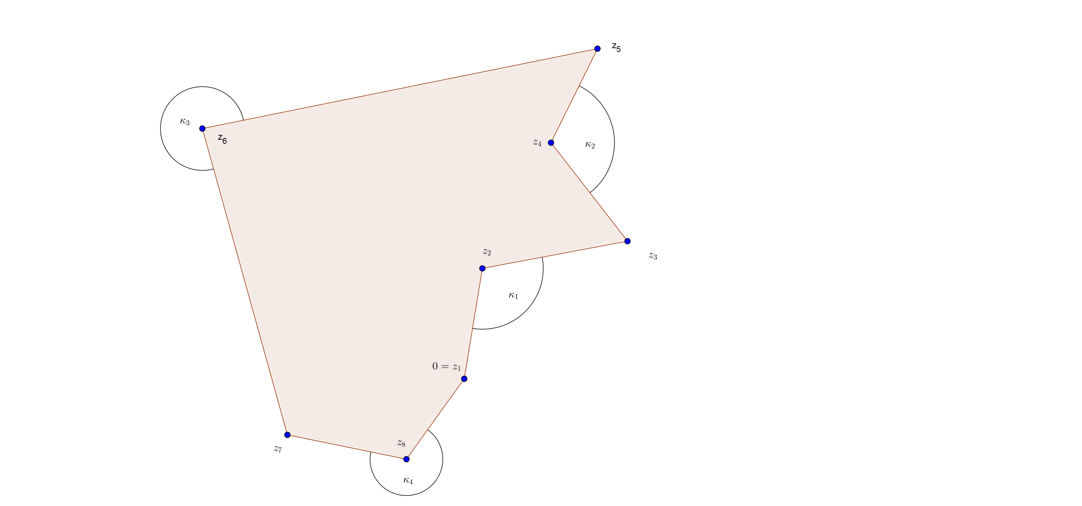
can be thought as the set of oriented polygons
Note that each element in has an outer angle at the vertex , , where the outer angle is the angle between the vectors and measured counter-clockwise. Also, for all and for all , . See Figure 2.
Remark 1.
Dimension of is since each element is determined by its coordinates .
3.1 The area Hermitian form and the formula for its signature
In this section we introduce the Hermitian form that we are interested in. Also we give the formula for its signature. Consider the Hermitian form
on , where . We know that if is a simple polygon, then the area of is just the square-norm of , . Therefore this form is called area Hermitian form.
We now state the formula that we prove. First, we introduce some notation.
Let
We denote the cardinality of a set by . Let
| (1) |
and
| (2) |
where is the floor function.
Lemma 1.
Let . Then
In particular, only depends on .
Proof.
Note that . The definition of implies that
Therefore, it follows that
since is equal to 0. The particular case is obvious.
∎
Lemma 2.
If is a permutation of and , then
Proof.
It is clear from the definition of that . Also Lemma 1 implies that . Since
it follows that for any permutation . ∎
We will prove that the signature of the area Hermitian is
that is, we will prove that
- 1.
;
- 2.
;
- 3.
.
Note that this will imply that is non-singular if and only if .
3.2 The case n=2
In this section we consider the case where . It follows that has dimension 1. This means that the polygons that we consider have 4 edges and we can easily draw them. See Figure 3.
Lemma 3.
If , then the signature of the area Hermitian form is .
Proof.
There are 3 cases to consider.
- 1.
. From the left of Figure 3, it is clear that the polygon corresponding to a non-zero element of has positive area. Since the area of the polygon corresponding to a non-zero element of is the square-norm of that element, we see that each non-zero element of has positive square-norm. Since is one-dimensional, it follows that the signature of the area Hermitian form is . On the other hand, it follows directly from the definition of that . The result follows.
- 2.
. In this case, every element in has area 0. See the middle of Figure 3 . Therefore, the signature is . Also, it is clear that .
- 3.
. In this case each polygon corresponding to a non-zero element is negatively oriented. This means that the orientation of these polygons is clockwise. Therefore, each non-zero element of this set has negative area. See the right hand side of Figure 3. It follows that the signature of the form is . Also, it is clear from the definition of and that and .
∎

3.3 A special family of polygons
In this section, we assume that , where the curvature data has length .
Lemma 4.
Let .
- 1.
If , then the signature of the area Hermitian form on is .
- 2.
If , then the signature of the area Hermitian form on is .
Proof.
The case was proven in Lemma 3. We will prove the lemma by induction on the length of curvature data , . Assume that . We start with a useful observation. Consider the map
which sends to itself. It is clear that this map is a vector space isomorphism. It simply gives a polygon the opposite orientation. Note that the following formula holds:
It follows that . Consider the following vector subspace of :
Note that is an -dimensional vector subspace. Also, consider the restriction of the area Hermition form on . It is easy to see that and are isomorphic as complex vector spaces with Hermitian forms.
Consider a basis for so that
- 1.
if ;
- 2.
if ;
- 3.
if ;
- 4.
and if .
Let
- 1.
be the vector subspace spanned by ;
- 2.
be the vector subspace spanned by ;
- 3.
be the vector subspace spanned by .
Assume that , . Then is -dimensional and the induction hypothesis implies that the signature of the area Hermitian form on is . Therefore
where and have dimension . Consider an element . Applying the Gram–Schmidt orthogonalization process if necessary, we can choose so that it is orthogonal to . Therefore the signature of the area Hermitian form on is
- 1.
,
- 2.
or
- 3.
.
Since , it follows that this signature is .
Assume that . Then is a dimensional subspace of . The induction hypothesis implies that the signature of the area Hermitian form on is . Therefore the dimension of is , the dimension of is and the dimension of is .
Take an element so that is orthogonal to and . We can assure this by the Gram–Schmidt orthogonalization process. Let be the vector space spanned by and . It is clear that
| (3) |
Assume that is orthogonal to , or equivalently, that the area Hermitian form restricted to is zero. Let
be a generator of . There is an integer such that for and . Note that . Consider the following element of :
where the first 1 is in the coordinate . Then
This is a contradiction. It follows that the area Hermitian form restricted to is not trivial. Therefore the signature of the area Hermitian form restricted to is
- 1.
,
- 2.
or
- 3.
.
Regarding the decomposition 3, it follows that the signature of on is
- 1.
,
- 2.
or
- 3.
.
Since , the signature is . ∎
The following corollary is an immediate application of Lemma 4.
Corollary 1.
If , then the signature of the area Hermitian form is .
Proof.
3.4 Cutting-Gluing Operations
In this section, we explain why for any permutation , and are isomorphic as complex vector spaces equipped with Hermitian forms.
We prove the claim by using some cutting and gluing operations. Before proceeding to the general case, we first introduce cutting and gluing operations on , where . We know that is 2-dimensional and that the signature of on it is . See Lemma 4. Take an element . Then
and
By abusing notation, we denote an element as . Now consider a positively oriented element . This element has positive square-norm, that is,
Recall that is the area of the corresponding polygon which actually is a triangle.
In Figure 4, consider the line segment and cut the triangle through this line segment to get two triangles. Glue the edges and by a rotation of angle around . In this way, we get another element in having the same area with coordinates . Therefore we have a map
sending . Clearly this map is a vector space isomorphism and we realized that it respects the area Hermitian form.

In general, even if the entries of the curvature data are not equal, we can use these cutting-gluing operations to find isomorphisms between and . Note that it is enough to consider the cases for which is a transposition to prove that and are isomorphic. Take an element , and consider it as a polygon in the complex plane. Assume that the line segment joining and does not intersect the polygon except at its endpoints. Cut the polygon through the line segment joining and . Glue the edge in the resulting quadrangle with the edge of the polygon to get the element . In this way, we get an area-preserving map from a subset of to , where . Note that this map extends to an area-preserving linear map between and . Indeed, this linear map is an isomorphism; one can reverse the cutting and gluing operations to get an inverse for the map. See Figure 5.

Therefore, we have proved the following lemma.
Lemma 5.
- 1.
For any , and are isomorphic as complex vector spaces equipped with Hermitian forms.
- 2.
The signature of the area Hermitian form on is equal to the signature of the area Hermitian form on .
Note that these cutting-gluing operations were introduced in [13].
3.5 Signature calculation
In this section we prove the signature formula. Let . Assume that and . Let
Also let . Consider the following dimensional subspace of :

A generic element of is shown in Figure 6. It is not difficult to see that together with the induced Hermitian form and are isomorphic. We want to find an orthogonal complement of in . In , there is a unique element of the form
Since the angle at the fourth vertex, , is , it follows that and
On the other hand, any element in is a constant multiple of an element of the form
It follows that
Let denote the vector space generated by . Clearly . Note that we have proved the following lemma.
Lemma 6.
If and , then .
Theorem 3.
The signature of the area Hermitian form for is . Also we have the following formulas for and :
and
where
Proof.
We prove the first part of the theorem by induction on . If we know that the statement is true. See Lemma 3. Assume that . If all of the are , then we know the theorem is true. See Corollary 1. Assume that not all of the are . It follows that there are , , such that . By Lemma 2 and Lemma 5, we may assume that .
Assume that . Note that Lemma 6 and the induction hypothesis on the vector spaces , imply that
And we also have
Therefore . Note that a similar calculation holds for the case .
The formulae for and follow easily from Lemma 1. ∎
Corollary 2.
Let .
- 1.
If , then the signature is .
- 2.
If , then the signature is .
- 3.
If , then the signature is .
- 4.
If , then the signature is .
- 5.
If , then the signature is .
- 6.
If , then the signature is .
Acknowledgments
The author is grateful to Susumu Tanabe, Muhammed Uludağ, Athanase Papadopoulos, Ke’nishi Ohshika and Haruko Nishi for their suggestions and help. He is financially supproted by TÜBİTAK.
References
- [1] A. Alexandrov, Convex polyhedra. Springer Monographs in Mathematics, Springer-Verlag, Berlin, 2005.
- [2] C. Bavard and É. Ghys, Polygones du plan et polyedres hyperboliques. Geometriae Dedicata 43.2 (1992), 207-224.
- [3] J. Fisher, D. Ruoff and J. Shilleto, Perpendicular polygons. The American Mathematical Monthly, 92.1 (1985), 23-37.
- [4] A. Gonzalez, J. Lopez-Lopez, Shapes of tetrahedra with prescribed cone angles. Conformal Geometry and Dynamics of the American Mathematical Society. 15.5 (2011), 50-63.
- [5] H. Groemer, Geometric applications of Fourier series and spherical harmonics. (Encyclopedia of Mathematics and its Applications). Cambridge University Press, Cambridge, 1996.
- [6] F. Fillastre, From spaces of polygons to spaces of polyhedra following Bavard, Ghys and Thurston. Enseignement Mathématique. 57.2 (2011), 23-56.
- [7] D. Hulin and M. Troyanov, Prescribing curvature on open surfaces. Mathematische Annalen. 293.1 (1992), 277-315.
- [8] I. Izmestiev, A simple proof of an isoperimetric inequality for Euclidean and hyperbolic cone-surfaces. Differential Geometry and its Applications 43 (2015), 95-101.
- [9] S. Kojima and Y. Yamashita, Shapes of stars. Proceedings of the American Mathematical Society 117.3 (1993), 845-851.
- [10] H. Nishi, On the signature of area form on the polygon space. Josai Mathematical Monographs. 6 (2013), 147-150
- [11] H. Nishi and K. Ohshika, A pseudo-metric on moduli space of hyperelliptic curves. Josai Mathematical Monographs, 5 (2012), 51-59.
- [12] H. Nishi and K. Ohshika, A parametrisation of Teichmüller spaces by polygons. Proceedings of NACA, 2011.
- [13] İ. Sağlam, Triangulations and quadrangulations of the sphere. International Journal of Mathematics. 26.8 (2015), 1550063.
- [14] İ. Sağlam, Ideal Triangulation and Disc Unfolding of a Singular Flat Surface. Turkish Journal of Mathematics. 45 (2021), 1635-1648.
- [15] İ. Sağlam, Complete flat cone metrics on punctured surfaces. Turkish Journal of Mathematics. 43 (2019), 813-832.
- [16] G. Tahar, Geometric triangulations and flips. Comptes Rendus Mathématique. 357.7 (2019), 620-623.
- [17] W. Thurston, Shapes of polyhedra and triangulations of the sphere. Geometry and Topology Monographs. 1 (1998) 511-549.
- [18] M. Troyanov, On the moduli space of singular Euclidean surfaces. In: Handbook of Teichmüller Theory (A. Papadopoulos, ed) Vol. I, EMS Publishing House, Zürich, 2007, 507-540.
- [19] M. Troyanov, Les surfaces euclidiennes à singularités coniques. L’Enseignement Mathématique, 32 (1986), 79-94.
- [20] M. Troyanov, Prescribing curvature on compact surfaces with conical singularities. Transactions of the American Mathematical Society. 324.2 (1991), 793-821.