Log Gaussian Cox processes on the sphere

Let $\mathbb{S}^{d}=\{x\in\mathbb{R}^{d+1}:\|x\|=1\}$ denote the $d$-dimensional unit sphere included in the $(d+1)$-dimensional Euclidean space $\mathbb{R}^{d+1}$, equipped with the usual inner product $\langle x,y\rangle=\sum_{i=0}^{d}x_{i}y_{i}$ for points $x=(x_{0},\ldots,x_{d}),y=(y_{0},\ldots,y_{d})\in\mathbb{R}^{d+1}$ and the usual length $\|x\|=\sqrt{\langle x,x\rangle}$. We are mainly interested in the case of $d=2$. By a region $U\subseteq\mathbb{S}^{d}$ we mean that $U$ is a Borel set. For unit vectors $u,v\in\mathbb{S}^{d}$, let $d(u,v)=\arccos(\langle u,v\rangle)$ be the geodesic distance on the sphere.

By a point process on $\mathbb{S}^{d}$, we understand a random finite subset X of $\mathbb{S}^{d}$. We say that X is isotropic if $O\textbf{X}$ is distributed as X for any $(d+1)\times(d+1)$ rotation matrix $O$. We assume that X has an intensity function, $\lambda(u)$, and a pair correlation function, $g(u,v)$, meaning that if $U,V\subseteq\mathbb{S}^{d}$ are disjoint regions and $N(U)$ denotes the cardinality of $X\cap U$, then

where $\mathrm{d}u$ is the Lebesgue/surface measure on $\mathbb{S}^{d}$. We say that X is (first order) homogeneous if $\lambda(u)=\lambda$ is constant, and second order intensity reweighted homogeneous if $g(u,v)=g(r)$ only depends on $r=d(u,v)$. Note that these properties are implied by isotropy of X, and second order intensity reweighted homogeneity allows to define the (inhomogeneous) $K$-function (Baddeley et al., 2000) by

for an arbitrary chosen point $u\in\mathbb{S}^{d}$, where $\mathrm{d}v$ denotes Lebesgue/surface measure on $\mathbb{S}^{d}$. For instance,

For a Poisson process $\mathbf{X}$ on $\mathbb{S}^{d}$ with intensity function $\lambda$, $N(\mathbb{S}^{d})$ is Poisson distributed with mean $\int\lambda(u)\,\mathrm{d}u$, and conditional on $N(\mathbb{S}^{d})$, the points in $\mathbf{X}$ are independent identically distributed with a density proportional to $\lambda$. The process is second order intensity reweighted homogeneous, with $K$-function

Let $\mathbf{Z}=\{\mathbf{Z}(u):u\in\mathbb{S}^{d}\}$ be a non-negative random field so that almost surely $\int\mathbf{Z}(u)\,\mathrm{d}u$ is well-defined and finite, and $Z(u)$ has finite variance for all $u\in\mathbb{S}^{d}$. We say that $\mathbf{X}$ is a Cox process driven by $\mathbf{Z}$ if $\mathbf{X}$ conditional on $\mathbf{Z}$ is a Poisson process on $\mathbb{S}^{d}$ with intensity function $\mathbf{Z}$. Then $\mathbf{X}$ has intensity function

and defining the residual driving random field by $\mathbf{Z}_{0}=\{\mathbf{Z}_{0}(u):u\in\mathbb{S}^{d}\}$, where $\mathbf{Z}_{0}(u)=\mathbf{Z}(u)/\lambda(u)$ (setting $0/0=0$), $\mathbf{X}$ has pair correlation function

Thus $\mathbf{X}$ is second order intensity reweighted homogeneous if $\mathbf{Z}_{0}$ is isotropic, that is, $\{\mathbf{Z}_{0}(Ou):u\in\mathbb{S}^{d}\}$ is distributed as $\mathbf{Z}_{0}$ for any $(d+1)\times(d+1)$ rotation matrix $O$. We shall naturally specify such Cox processes in terms of $\lambda$ and $\mathbf{Z}_{0}$.

Figure 1(a) shows the sky positions of 10,546 galaxies from the Revised New General Catalogue and Index Catalogue (RNGC/IC) (Steinicke, 2015). Here, we are following Lawrence et al. (2016) in making a rotation of the original data so that the two circles limit a band around the equator, which is an approximation of the part of the sky obscured by the Milky Way, and the observation window $W\subset\mathbb{S}^{2}$ is the complement of the band; 64 galaxies contained in the band are omitted.

Different plots and tests in the accompanying supporting information to Lawrence et al. (2016) clearly show that the galaxies are aggregated and not well-described by an inhomogeneous Poisson process model. Lawrence et al. (2016) fitted the intensity function

where $u=(\sin\theta\cos\phi,\sin\theta\sin\phi,\cos\theta)$, $\theta\in[0,\pi]$ is the colatitude, and $\phi\in[0,2\pi)$ is the longitude. The term $-0.112\sin\theta\cos\phi-0.149\sin\theta\sin\phi+0.320\cos\theta$ is the inner product of $u$ with $(-0.112,-0.149,0.32)$, and the term $1.971\cos^{2}\theta$ allows a gradient in intensity from the poles to the equator, cf. the discussion in Lawrence et al. (2016) and their plot Movie 2 (where we recommend using the electronic version of the paper and the link in the caption to this plot). Throughout this paper, we also use (5).

Lawrence et al. (2016) proposed an inhomogeneous Thomas process, that is, a Cox process with intensity function (5) and isotropic residual driving random field given by

where $\mathbf{Y}$ is a homogeneous Poisson process on $\mathbb{S}^{2}$ with intensity $\kappa>0$, and where

is the density for a von Mises-Fisher distribution on $\mathbb{S}^{2}$ with mean direction $y$ and concentration parameter $\xi>0$. They estimated $\kappa$ and $\eta$ by a minimum contrast procedure (Diggle and Gratton, 1984; Diggle, 2013), where a non-parametric estimate $\widehat{K}$ is compared to

Specifically, the minimum contrast estimate $(\hat{\kappa},\hat{\eta})$ is minimising the contrast

where $b>a\geq 0$ are user-specified parameters. Lawrence et al. (2016) used the integration interval $[a,b]=[0,1.396]$, where 1.396 is the maximal value of the smallest distance from the north pole respective south pole to the boundary of $W$. They obtained $\hat{\kappa}=5.64$ and $\hat{\xi}=266.6$.

Let $\mathbf{Y}=\{\mathbf{Y}(u):u\in\mathbb{S}^{d}\}$ be a Gaussian random field (GRF), that is, $\sum_{i=1}^{n}a_{i}\mathbf{Y}(u_{i})$ is normally distributed for any integer $n>0$, numbers $a_{1},\ldots,a_{n}$, and $u_{1},\ldots,u_{n}\in\mathbb{S}^{d}$. Let $\mu(u)=\mathrm{E}\mathbf{Y}(u)$ be its mean function and $c(u,v)=\mathrm{E}[(\mathbf{Y}(u)-\mu(u))(\mathbf{Y}(v)-\mu(v))]$ its covariance function. Assuming that almost surely $\mathbf{Z}:=\exp(\mathbf{Y})$ is integrable, the Cox process $\mathbf{X}$ driven by $\mathbf{Z}$ is called a log Gaussian Cox process (Møller et al., 1998; Møller and Waagepetersen, 2004, LGCP;).

Define the corresponding mean-zero GRF, $\mathbf{Y}_{0}:=\mathbf{Y}-\mu$, which has also covariance function $c$. Assuming $\mu$ is a Borel function with an upper bounded, then almost sure continuity of $\mathbf{Z}_{0}$ implies almost sure integrability of $\mathbf{Z}=\mathbf{Z}_{0}\exp(\mu)$, and so $\mathbf{X}$ is well-defined. In turn, almost sure continuity of $\mathbf{Z}_{0}$ is implied if almost surely $\mathbf{Y}_{0}$ is locally sample Hölder continuous of some order $k>0$, which means the following: With probability one, for every $s\in\mathbb{S}^{d}$, there is a neighbourhood $V$ of $s$ and a constant $C_{V,k}$ so that

The following proposition is a special case of Lang et al. (2016, Corollary 4.5), and it provides a simple condition ensuring (8).

The following proposition is easily verified along similar lines as Proposition 5.4 in Møller and Waagepetersen (2004) using (3)-(4) and the expression for the Laplace transform of a normally distributed random variable.

In other words, the distribution of $\mathbf{X}$ is specified by $(\lambda,g)$ because $\mu(u)=\log\lambda(u)-\log g(u,u)/2$ and $c(u,v)=\log g(u,v)$ specify the distribution of the GRF.

By (10), second order intensity reweighted homogeneity of the LGCP is equivalent to isotropy of the covariance function, that is, $c(u,v)=c(r)$ depends only on $r=d(u,v)$. Parametric classes of isotropic covariance functions on $\mathbb{S}^{d}$ are provided by Gneiting (2013), see Table 2 in Section 4.1, and by Møller et al. (2018). In Section 3.3, we consider the so-called multiquadric covariance function which is isotropic and given by

where $(\sigma,\delta,\tau)\in(0,\infty)\times(0,1)\times(0,\infty)$.

In fact locally sample Hölder continuity is satisfied when considering other commonly used parametric classes of covariance functions, but the proof will be case specific as shown in the proof of Proposition 4 in Section 4.1.

In this section, to see how well the estimated Thomas process, $\mathbf{X}_{\mathrm{Thom}}$, obtained in Lawrence et al. (2016) fits the sky positions of galaxies discussed in Section 2.3, we use methods not involving the $K$-function (or the related pair correlation function, cf. (1)) because it was used in the estimation procedure.

The point pattern in Figure 1(b) was obtained by an independent thinning procedure of the point pattern in Figure 1(a), with retention probability $\lambda_{\mathrm{min}}/\lambda(u)$ at location $u\in W$, where $\lambda(u)$ is given by (5) and $\lambda_{\mathrm{min}}:=\inf_{u\in\mathbb{S}^{2}}\lambda(u)$. If we imagine a realization of $\mathbf{X}_{\mathrm{Thom}}$ on $\mathbb{S}^{2}$ could had been observed so that the independent thinning procedure could had taken place on the whole sphere, then the corresponding thinned Thomas process, $\mathbf{X}_{\mathrm{thinThom}}$, is isotropic. Thus the commonly used $F,G,J$-functions would apply: Briefly, for a given isotropic point process $\mathbf{X}$ on $\mathbb{S}^{d}$, an arbitrary chosen location $u\in\mathbb{S}^{d}$, and $r\in[0,\pi]$, by definition $F(r)$ is the probability that $\mathbf{X}$ has a point in a cap $C(u,r)$ with center $u$ and geodesic distance $r$ from $u$ to the boundary of the cap; $G(r)$ is the conditional probability that $\mathbf{X}\setminus\{u\}$ has a point in $C(u,r)$ given that $u\in\mathbf{X}$; and $J(r)=(1-G(r))/(1-F(r))$ when $F(r)<1$. For the empirical estimates of the $F,G,J$-functions, as we only observe points within the subset $W\subset\mathbb{S}^{2}$ specified in Section 2.3, edge correction factors will be needed, where we choose to use the border-corrected estimates from Lawrence et al. (2016).

Empirical estimates $\widehat{F},\widehat{G},\widehat{J}$ can then be used as test functions for the global rank envelope test, which is supplied with graphical representations of global envelopes for $\widehat{F},\widehat{G},\widehat{J}$ as described in Myllymäki et al. (2017). As we combined all three test functions as discussed in Mrkvic̆ka et al. (2016) and Mrkvic̆ka et al. (2017), we followed their recommendation of using $3\times 2499=7497$ simulations of $\mathbf{X}_{\mathrm{thinThom}}$ for the calculation of $p$-values and envelopes. Briefly, under the claimed model, with probability 95% we expect $\widehat{F},\widehat{G},\widehat{J}$ (the solid lines in Figure 2(a)–2(c)) to be within the envelope (either the dotted or dashed lines in Figure 2(a)–2(c) depending on the choice of $[a,b]$ as detailed below), and the envelope corresponds to a so-called global rank envelope test at level 5%. In Table 1, the limits of the $p$-intervals correspond to liberal and conservative versions of the global rank envelope test (Myllymäki et al., 2017). Table 1 and Figure 2(a)–2(c) clearly show that the estimated Thomas process is not providing a satisfactory fit no matter if in the contrast (7) the long integration interval $[a,b]=[0,1.396]$ from Lawrence et al. (2016) or the shorter interval $[a,b]=[0,0.175]$ (corresponding to 0-10 degrees) is used for parameter estimation. When $[a,b]=[0,0.175]$, larger estimates $\hat{\kappa}=6.67$ and $\hat{\xi}=353.94$ are obtained as compared to $\hat{\kappa}=5.64$ and $\hat{\xi}=266.6$ from Lawrence et al. (2016). Note that the $p$-values and envelopes are not much affected by the choice of integration interval in the minimum contrast estimation procedure, cf. Table 1 and Figure 2(a)–2(c). The envelopes indicate that at short inter-point distances $r$, there is more aggregation in the data than expected under the two fitted Thomas processes.

We also fitted an inhomogeneous LGCP, $\mathbf{X}_{\mathrm{LGCP}}$, still with intensity function given by (5) and with multiquadric covariance function as in (11). The same minimum contrast procedure as above was used except of course that in the contrast given by (7), the theoretical $K$-function was obtained by combining (1), (10), and (11), where numerical calculation of the integral in (1) was used. The estimates are $(\hat{\sigma}^{2},\hat{\delta},\hat{\tau})=(4.50,0.99,0.25)$ if $[a,b]=[0,0.175]$ is the integration interval, and $(\hat{\sigma}^{2},\hat{\delta},\hat{\tau})=(1.30,0.87,2.03)$ if $[a,b]=[0,1.396]$. For each choice of integration interval, Figure 3 shows the estimated log pair correlation function, that is, the estimated covariance function of the underlying GRF, cf. (10). Comparing the two pair correlation functions, the one based on the short integration interval is much larger for very short inter-point distances $r$, then rather similar to the other at a short interval of $r$-values, and afterwards again larger, so the fitted LGCP using the short integration interval is more aggregated than the other case. Further, Figure 4 shows the empirical $K$-function and the fitted $K$-functions for both the Thomas process and the LGCP when using the different integration intervals (for ease of comparison, we have subtracted $K_{\mathrm{Pois}}$, the theoretical $K$-function for a Poisson process, cf. (2)). The fitted $K$-functions are far away from the empirical $K$-function for large values of $r$. However, having a good agreement for small and modest values of $r$ is more important, because the variance of the empirical $K$-function seems to be an increasing function of $r$ and the interpretation of the $K$-function becomes harder for large $r$-values. For small and modest $r$-values, using the LGCP model and the short integration interval provides the best agreement between the empirical $K$-function and the theoretical $K$-function, even when $r$ is outside the short integration interval.

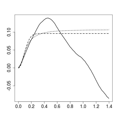
Table 1 and Figure 2(d)–2(f) show the results for the fitted LGCPs when making a model checking along similar lines as for the fitted Thomas processes (i.e., based on a thinned LGCP and considering the empirical $F,G,J$-functions together with global envelopes). Table 1 shows that the fitted LGCP based on the long integration interval gives an interval of similar low $p$-values as for the fitted Thomas process in Lawrence et al. (2016), and Figure 2(e)–2(f) indicate that the data is more aggregated than expected under this fitted LGCP. Finally, the fitted LGCP based on the short integration interval gives $p$-values of about 24%, and the empirical curves of the functional summary statistics appear in the center of the envelopes, cf. Figure 2(d)–2(f).

Finally, we have studied how sensible the results will be when using the independent thinning procedure. Figure 5 is similar to Figure 2 except that the 1000 solid lines show the empirical estimates $\widehat{F},\widehat{G},\widehat{J}$ when we repeat the thinning procedure 1000 times. The empirical estimates do not vary much in the 1000 cases. Moreover, Figure 6 is similar to Table 1 and shows the intervals for $p$-values obtained in the 1000 cases. The intervals for the fitted Thomas process, using the short or long integration interval, and for the fitted LGCP, using the long integration interval, are effectively not varying in the 1000 cases (the three lower solid curves correspond to liberal $p$-values and visually they appear as one curve which is close to 0: the curve in the LGCP case varies around $10^{-4}$, and the two curves in the Thomas process case vary around $4\times 10^{-4}$). The intervals for the fitted LGCP, using the short integration interval, are much shorter than for the three other fitted models, and they vary from 0.75% - 0.77% to 41.44% - 41.48%, with only 12 out of the 1000 intervals below the 5% level. Thus, the results are not so sensitive to the independent thinning procedure and the conclusion, namely that the fitted LGCP, using the short integration interval, is fitting well whilst the other fitted models do not, is almost the same in the 1000 cases.

As noticed in Section 3.1, under mild conditions for the mean function $\mu$, almost sure locally sample Hölder continuity of the mean-zero GRF $\mathbf{Y}_{0}=\mathbf{Y}-\mu$ is a sufficient condition for establishing the existence of a LGCP driven by $\exp(\mathbf{Y})$. In turn, almost sure locally sample Hölder continuity of $\mathbf{Y}_{0}$ is implied by the condition (9) in Proposition 1, and Proposition 3 states that the multiquadric covariance function is satisfying this condition. As shown in the following proposition, (9) is satisfied for any of the parametric classes of isotropic covariance functions on $\mathbb{S}^{d}$ given by Gneiting (2013), see Table 2. In brief, these are the commonly used isotropic covariance functions which are expressible on closed form.

As demonstrated, a LGCP on the sphere possesses useful theoretical properties, in particular moment properties as provided by Proposition 2. We exploited these expressions for the intensity and pair correlation function when dealing with the inhomogeneous $K$-function, which concerns the second moment properties of a second order intensity reweighted homogeneous point process.

Proposition 2 extends as follows. For a general point process on $\mathbb{S}^{d}$, the $n$-th order pair correlation function $g(u_{1},\ldots,u_{n})$ is defined for integers $n\geq 2$ and multiple disjoint regions $U_{1}\ldots,U_{n}\subseteq\mathbb{S}^{d}$ by

provided this multiple integral is well-defined and finite. The following proposition follows immediately as in Møller and Waagepetersen (2003, Theorem 1).

Higher-order pair correlation functions as given by (16) may be used for constructing further functional summaries e.g. along similar lines as the third-order characteristic studied in Møller et al. (1998) and the inhomogeneous $J$-function studied in Cronie and van Lieshout (2015, Section 5.3).

It would also be interesting to exploit the following result for the reduced Palm distribution of a LGCP on the sphere as discussed in Coeurjolly et al. (2017) in the case of LGCPs on $\mathbb{R}^{d}$. Intuitively, the reduced Palm distribution of a point process $\mathbf{X}$ on $\mathbb{S}^{d}$ at a given point $u\in\mathbb{S}^{d}$ corresponds to the distribution of $\mathbf{X}\setminus\{u\}$ conditional on that $u\in\mathbf{X}$; see Lawrence et al. (2016) and Møller and Rubak (2016). Along similar lines as in Coeurjolly et al. (2017, Theorem 1), we obtain immediately the following result.

Bayesian analysis of inhomogeneous LGCPs on the sphere has previously been considered in Simpson et al. (2016) using the R-INLA approach: Their covariance model for the underlying GRF is an extension of the Matérn covariance function defined as the covariance function at any fixed time to the solution to a stochastic partial differential equation which is stationary in time and isotropic on the sphere. Using the R-INLA approach, a finite approximation of their LGCP based on a triangulation of the sphere is used, which for computational efficiency requires $\alpha:=\nu+d/2$ to be an integer, where $\nu>0$ is the shape parameter (the expression $\alpha=\nu-d/2$ in their paper is a typo). Simpson et al. (2016) considered an inhomogeneous LGCP defined only on the world’s oceans, with $d=2$ and $\alpha=2$, so $\nu=1$. In the original Matérn model (Gneiting, 2013, Table 1), $0<\nu\leq 0.5$ and the covariance function has a nice expression in term of a Bessel function, but otherwise the covariance function can only be expressed by an infinite series in terms of spherical harmonics (Simpson, 2009, Section 6.4). In contrast, we have focused on covariance functions $c$ which are expressible on closed form so that we can easily work with the pair correlation function $g=\exp(c)$. Indeed it could be interesting to apply the R-INLA approach as well as other likelihood based methods of inference (Møller and Waagepetersen, 2017), though they are certainly much more complicated than the simple inference procedure considered in the present paper.

For comparison with the analysis of the sky positions of galaxies in Lawrence et al. (2016), we used a minimum contrast estimation procedure, but other simple and fast methods such as composite likelihood (Guan, 2006; Møller and Waagepetersen, 2017, and the references therein) could have been used as well. It is well-known that such estimation procedures can be sensitive to the choice of user-specified parameters. We demonstrated this for the choice of integration interval in the contrast, where using a short interval and an inhomogeneous LGCP provided a satisfactory fit, in contrast to using an inhomogeneous Thomas process or a long interval. It could be interesting to use more advanced estimation procedures such as maximum likelihood and Bayesian inference. This will involve a time-consuming missing data simulation-based approach (Møller and Waagepetersen, 2004; Møller and Waagepetersen, 2017, and the references therein).

The Thomas process is a mechanistic model since it has an interpretation as a cluster point process (Lawrence et al., 2016). The original Thomas process in $\mathbb{R}^{3}$ (i.e., using a 3-dimensional isotropic zero-mean normal distribution as the density for a point relative to its cluster centre) may perhaps appear natural for positions of galaxies in the 3-dimensional space – but we question if the Thomas process from Lawrence et al. (2016) is a natural model for the sky positions because these points are obtained by projecting clusters of galaxies in space to a sphere which may not produce a clear clustering because of overlap. Rather, we think both the inhomogeneous Thomas and the inhomogeneous LGCP should be viewed as empirical models for the data. Moreover, it could be investigated if the Thomas process replaced by another type of Neyman-Scott process (Neyman and Scott, 1958; Neyman and Scott, 1972) or a (generalised) shot noise Cox process (Møller, 2003; Møller and Torrisi, 2005) would provide an adequate fit.

As a specific model, we only considered the multiquadric covariance function for the underlying GRF of the LGCP. A more flexible model could be the spectral model studied in Møller et al. (2018), where a parametric model for the eigenvalues of the spectral representation of an isotropic covariance function $c(r)$ ($r\geq 0$) in terms of spherical harmonics is used (incidentally, the eigenvalues are also known for the multiquadric covariance function if $\tau=1/2$). The spectral representation allows a Karhunen-Loève representation which could be used for simulation. However, for the data analysed in this paper, we found it easier and faster just to approximate the GRF $\mathbf{Y}=\{\mathbf{Y}(u):u\in\mathbb{S}^{2}\}$, using a finite grid $I\subset\mathbb{S}^{2}$ so that each $\mathbf{Y}(u)$ is replaced by $\mathbf{Y}(v)$ if $v$ is the nearest grid point to $u$, and using the singular value decomposition when simulating the finite random field $\{\mathbf{Y}(v):v\in I\}$. When using spherical angles $(\theta,\psi)$ as in (5), a regular grid over $[0,\pi]\times[0,2\pi)$ can not be recommended, since the density of grid points will large close to the poles and small close to equator. Using a regular grid $I\subset\mathbb{S}^{2}$ avoids this problem, nonetheless, there are only five regular grids on the sphere (Coxeter, 1973). We used a nearly-regular grid consisting of 4098 points on the sphere (Szalay et al., 2007, and the references therein) and computed using the R package mvmesh (Nolan, 2016).

References

- Baddeley et al. (2000) A. J. Baddeley, J. Møller, and R. Waagepetersen. Non- and semi-parametric estimation of interaction in inhomogeneous point patterns. Statistica Neerlandica, 54:329–350, 2000.
- Coeurjolly et al. (2017) J.-F. Coeurjolly, J. Møller, and R. Waagepetersen. Palm distributions for log Gaussian Cox processes. Scandinavian Journal of Statistics, 44:192–203, 2017.
- Coxeter (1973) H. S. M. Coxeter. Regular Polytopes. Methuen, London, 1973.
- Cronie and van Lieshout (2015) O. Cronie and M. N. M. van Lieshout. A -function for inhomogeneous spatio-temporal point processes. Scandinavian Journal of Statistics, 42:562–579, 2015.
- Diggle (2013) P. J. Diggle. Statistical Analysis of Spatial and Spatio-temporal Point Patterns. CRC Press, Boca Raton, 2013.
- Diggle and Gratton (1984) P. J. Diggle and R. J. Gratton. Monte Carlo methods of inference for implicit statistical models. Journal of the Royal Statistical Society: Series B (Statistical Methodology), 46:193–227, 1984.
- (7) DLMF. NIST Digital Library of Mathematical Functions. http://dlmf.nist.gov/, Release 1.0.18 of 2018-03-27. URL http://dlmf.nist.gov/. F. W. J. Olver, A. B. Olde Daalhuis, D. W. Lozier, B. I. Schneider, R. F. Boisvert, C. W. Clark, B. R. Miller and B. V. Saunders, eds.
- Gneiting (2013) T. Gneiting. Strictly and non-strictly positive definite functions on spheres. Bernoulli, 19:1327–1349, 2013.
- Guan (2006) Y. Guan. A composite likelihood approach in fitting spatial point process models. Journal of the American Statistical Association, 101:1502–1512, 2006.
- Lang et al. (2016) A. Lang, J. Potthoff, M. Schlather, and D. Schwab. Continuity of random fields on Riemannian manifolds. Manuscript available at arXiv: 1607.05859, 2016.
- Lawrence et al. (2016) T. Lawrence, A. Baddeley, R. K. Milne, and G. Nair. Point pattern analysis on a region of a sphere. Stat, 5:144–157, 2016.
- Møller (2003) J. Møller. Shot noise Cox processes. Advances in Applied Probability, 35:614–640, 2003.
- Møller and Rubak (2016) J. Møller and E. Rubak. Functional summary statistics on the sphere with an application to determinantal point processes. Spatial Statistics, 18:4–23, 2016.
- Møller and Torrisi (2005) J. Møller and G. Torrisi. Generalised shot noise Cox processes. Advances in Applied Probability, 37:48–74, 2005.
- Møller and Waagepetersen (2017) J. Møller and R. Waagepetersen. Some recent developments in statistics for spatial point patterns. Annual Review of Statistics and Its Applications, 4:317–342, 2017.
- Møller and Waagepetersen (2003) J. Møller and R. P. Waagepetersen. Spatial Statistics and Computational Methods, chapter An introduction to simulation-based inference for spatial point processes, pages 37–60. Lecture Notes in Statistics 173, Springer-Verlag, New York, 2003.
- Møller and Waagepetersen (2004) J. Møller and R. P. Waagepetersen. Statistical Inference and Simulation for Spatial Point Processes. Boca Raton, FL, Chapman & Hall/CRC., 2004.
- Møller et al. (1998) J. Møller, R. Waagepetersen, and A. R. Syversveen. Log Gaussian Cox processes. Scandinavian Journal of Statistics, 25:451–482, 1998.
- Møller et al. (2018) J. Møller, M. Nielsen, E. Porcu, and E. Rubak. Determinantal point process models on the sphere. Bernoulli, 24:1171–1201, 2018.
- Mrkvic̆ka et al. (2016) T. Mrkvic̆ka, S. Soubeyrand, M. Myllymäki, P. Grabarnik, and U. Hahn. Monte Carlo testing in spatial statistics, with applications to spatial residuals. Spatial Statistics, 18:40–53, 2016.
- Mrkvic̆ka et al. (2017) T. Mrkvic̆ka, M. Myllymäki, and U. Hahn. Multiple Monte Carlo testing, with applications in spatial points. Statistics and Computing, 27:1239–1255, 2017.
- Myllymäki et al. (2017) M. Myllymäki, T. Mrkvic̆ka, P. Grabarnik, H. Seijo, and U. Hahn. Global envelope tests for spatial processes. Journal of the Royal Statistical Society: Series B (Statistical Methodology), 79:381–404, 2017.
- Neyman and Scott (1958) J. Neyman and E. L. Scott. Statistical approach to problems of cosmology. Journal of the Royal Statistical Society: Series B (Statistical Methodology), 20:1–43, 1958.
- Neyman and Scott (1972) J. Neyman and E. L. Scott. Processes of Clustering and Applications. John Wiley & Sons, New York, Stochastic Processes in Lewis PAW edition, 1972.
- Nolan (2016) J. P. Nolan. An R package for modeling and simulating generalized spherical and related distributions. Journal of Statistical Distributions and Applications, 3:3–14, 2016.
- Raskin (1994) R. G. Raskin. Spatial analysis on the sphere: a review, 1994. NGCIA technical report. (Available from http://eprints.cdlib.org/uc/item/5748n2xz). [Accessed February 1, 2018].
- Ripley (1976) B. D. Ripley. The second-order analysis of spatial point processes. Journal of Applied Probability, 13:255–266, 1976.
- Ripley (1977) B. D. Ripley. Modelling spatial patterns (with discussion). Journal of the Royal Statistical Society: Series B (Statistical Methodology), 39:172–212, 1977.
- Robeson et al. (2014) S. M. Robeson, A. Li, and C. Huang. Point-pattern analysis on the sphere. Spatial Statistics, 10:76–86, 2014.
- Simpson (2009) D. Simpson. Krylov Subspace Methods for Approximating Functions of Symmetric Positive Definite Matrices with Applications to Applied Statistics and Anomalous Diffusion. PhD thesis, Queensland University of Technology, 2009.
- Simpson et al. (2016) D. Simpson, J. B. Illian, F. Lindgren, S. H. Sørbye, and H. Rue. Going off grid: computationally efficient inference for log-Gaussian Cox processes. Biometrika, 103:49–70, 2016.
- Steinicke (2015) W. Steinicke. Revised new general catalogue and index catalogue, 2015. (Available from http://www.klima-luft.de/steinicke/index.htm). [Accessed February 1, 2018].
- Szalay et al. (2007) A. S. Szalay, J. Gray, G. Fekete, P. Z. Kunszt, P. Kukol, and A. Thakar. Indexing the sphere with the hierarchical triangular mesh. Manuscript available at arXiv: 0701164, 2007.