Binary Fluid Mixtures Computational methods in fluid dynamics Computational simulations of molecular and particle dynamics Phase transitions
Hydrodynamics of Binary Fluid Mixtures—An Augmented Multiparticle Collison Dynamics Approach
Abstract
The Multiparticle Collision Dynamics technique (MPC) for hydrodynamics simulations is generalized to binary fluid mixtures and multiphase flows, by coupling the particle-based fluid dynamics to a Ginzburg-Landau free-energy functional for phase-separating binary fluids. To describe fluids with a non-ideal equation of state, an additional density-dependent term is introduced. The new approach is verified by applying it to thermodynamics near the critical demixing point, and interface fluctuations of droplets. The interfacial tension obtained from the analysis of the capillary wave spectrum agrees well with the results based on the Laplace-Young equation. Phase-separation dynamics follows the Lifshitz-Slyozov law.
pacs
47.11.-jpacs
83.10.Rspacs
05.70.Fh1 Introduction
The description and modeling of multi-component and particle-laden flows is among the prime tasks of fluid-dynamics approaches and simulations. As a consequence, mesoscale hydrodynamics simulation techniques have seen an enormous surge in interest, development, and applications during the last decades. This was stimulated, on the one hand, by the easy and straightforward coupling with nano- or micro-particles in the fluid, and thus the possibility for the simulation of complex fluids, and, on the other hand, the natural incorporation of thermal fluctuations, which are essential, for example, for the conformations of flexible polymers under flow.
For the lattice Boltzmann method (LBM), an approach to simulate flows with multiple phases and components has already been suggested in the early 1990s by Gunstensen et al. [1] and Shan and Chen [2, 3], and has been applied very successfully since then. In this approach, the interaction between particles is described by a pseudopotential. The method is only consistent with thermodynamic theories when the dependence of the pseudopotential on the local density takes a special exponential form [3]. This limits the accessible equations of state to be addressed. An alternative approach has been suggested by Yeomans and collaborators a few years later for non-ideal fluids [4] and for binary-fluid mixtures [5]. This description is based on a free-energy functional, which enters the model via the local pressure tensor. This approach has the advantage that any desired free-energy functional can be employed. For dissipative particle dynamics (DPD), the description of multi-component fluids is rather straightforward, since there is an explicit conservative interaction between particles, which is taken to be more repulsive for particles of unlike species [6].
In contrast, the development of algorithms for multi-phase flows lags behind for a third popular mesoscale simulation technique, multiparticle collision dynamics (MPC) [7, 8]. This method has a priori no direct interactions between particles. Instead, it consists of alternating streaming and collision steps. In the collision step, particles are sorted into the cells of a simple cubic lattice. All particles in a given cell subsequently collide by exchanging momentum such that the total momentum is conserved. This is achieved, for example, by a rotation of the particle momenta in a comoving reference frame around a randomly oriented axis. This approach has been adapted to multi-phase hydrodynamics by modifying the collision rule. This is achieved by a collision operator that mimics an effective repulsive interaction between different particles species [9, 10, 11, 12, 13, 14]. For two-dimensional systems, the approach of Ref. [11] is thermodynamically consistent and yields the expected phase behavior, e.g., droplet formation [12]. An effective repulsive interaction has also been employed recently in a three-dimensional system to study the flow of emulsion droplets in non–wetting microchannels, the apparent contact angle of sessile droplets in mechanical equilibrium, and the dewetting of a liquid film from a wetting stripe [13], or the phase separation of binary fluids [14]. However, the latter approach shares the difficulty of the pseudo-potential LBM that there is no inherent consistency with thermodynamics.
Therefore, it would be highly desirable to have a free-energy based MPC method for non-ideal fluids and fluid mixtures, in a similar spirit than the free-energy based LBM described above. We develop such an approach in this paper, and verify its validity by applying it to phase separation near a critical point, the Young-Laplace equation for fluid droplets, and the interface profile between two coexisting phases. The advantage of the method is its applicability to a large variety of systems with different free-energy functionals.
2 Model
The MPC fluid is described by point particles of mass , which move in continuous space with continuous velocities and interact with each other by a stochastic process [15, 7, 8]. The dynamics of the particles proceeds in alternating streaming and collision steps. For a bare MPC fluid, i.e., without an external force, the streaming motion is ballistic and the particle positions , , are updated according to
| (1) |
where is the collision time and the are the particle velocities. Temperature is defined here by the average kinetic energy, i.e., in spatial dimensions; is the Boltzmann factor. In the collision step, the system is partitioned into cubic cells of side length , which define the local collision environment. Momentum exchange between the particles of a collision cell is achieved by a rotation of their relative velocities around a randomly oriented axis by an angle , where is the center-of-mass velocity of the particles in the particular cell. The MPC-particle velocities are then given by
| (2) |
Here, is the unit matrix and denotes the rotation operator. The orientation of the rotation axis is chosen randomly for every collision step and collision cell [7, 8]. The algorithm conserves particle number, energy and local momentum, and thus gives rise to long-range hydrodynamics [16]. The discretization implies a violation of Galilean invariance, which is reestablished by the random shift of the collision-cell lattice [17]. It is important to emphasize that the MPC fluid has the equation of state of an ideal gas, i.e., .
With a particle-based simulation approach, binary mixtures and their phase behavior can straightforwardly be studied by introducing a suitable pair-wise interaction between the two types of particles. However, such an approach would eliminate the main advantage of high computational efficiency of the MPC approach. In order to preserve the simplicity of this algorithm, we couple the dynamics of the MPC particles to the free-energy functional of a phase-separating system via the pressure tensor [5].
We consider a binary-fluid MPC system and divide the particles into particles of type and particles of type . Our starting point for the description of the interactions is the Ginzburg-Landau free-energy functional of a binary fluid,
| (3) |
where is the mass density and the order parameter, with average densities and . Hence, our approach corresponds to Model H and belongs to the Ising universality class [18, 19]. Phase separation is determined by the parameter , which (in the mean-field approximation) can be identified with the reduced temperature, i.e., , where is the critical temperature. The mass-density dependent term is added to the free-energy functional to control the fluid compressibility. From Eq. (3), the pressure tensor can be derived [20, 5, 21],
| (4) |
where refer to the Cartesian components and
| (5) | ||||
| (6) | ||||
| (7) |
We denote the first term as “bulk” and the second as “interfacial” term. The third term is related to the fluid equation of state and compressibility. In the following, we use , which leads to an ideal-gas-like pressure tensor . The isothermal compressibility of the fluid is then given by . Hence, the parameter can be varied to modify the fluid compressibility. Alternatively, also a non-linear state function can be used, e.g., , leading to the pressure tensor
| (8) |
Thereby, determines the strength of the fluid compressibility. We like to emphasize that also other expressions for can be employed for this purpose.
On the collision-cell level, the pressure gradients can equally well be written as body-force density acting on the fluid. We discretise the field variables and on the collision-cell level and in each of the MPC cells. From Eqs. (5)-(7), we can derive an expression for the force acting on the individual particles, which we split according to the three pressure contributions into . We discretize the bulk and compressibility contributions and by averaging over two neighbouring cells. As a consequence, while the scalar field variables and are defined in the collision cells, the vector quantities and are defined on the edges of the collision cells. As an example, the force in -direction is given by
| (9) | ||||
| (10) |
Equation (10) is the force due to an ideal-gas-like term. Similarly, the non-ideal-gas expression can be used, with the discretization .
For the interfacial contribution, , we apply a simple central difference scheme, i.e., , which leads to
| (11) |
The total forces in -direction on particles of type and in cell (,) are then
The proposed discretization scheme guarantees that the sum of forces is globally equal to zero. A more detailed derivation of the employed discretization scheme is presented in Appendix A. Finally, the modified streaming step is
| (12) | ||||
| (13) |
where the are given by the corresponding expressions for particles of type or .
Temperature of the system is maintained by applying a cell-level canonical thermostat, where the relative velocities are scaled within a collision cell and the scaling factor is determined from the distribution of the kinetic energy in the cell [22].

3 Two-dimensional systems
Order parameter and critical exponent. Depending on the parameters of the bulk free-energy density in Eq. (3), the binary fluid phase-separates into an -rich and a -rich phase (cf. Fig. 1). As is well-known from the Landau (or mean-field) theory (), phase separation occurs for (double-well potential) with the critical value at . Since we are taking thermal fluctuations and local field gradients into account, we expect a somewhat shifted value, with . In the vicinity of continuous phase transitions, the order parameter exhibits a power-law dependence of the form [23, 24]
| (14) |
with critical exponent and critical-temperature shift . Landau theory predicts the critical exponent , while the exact solution of the 2D Ising-model yields [23, 25].
To study the critical behavior of our A-B mixture, we employ a two-dimensional system with a box length , and an average particle number per collision cell of . The measured temperature is increased by approximately as a consequence of the additional forces by the coupling of the MPC fluid to the order parameter field. Further, we set the particle fractions to . The collision step, as for all the following 2D simulations, is performed with a rotation angle of and the collision time . For the phase diagram, the reduced-temperature parameter in the Ginzburg-Landau expression is varied within the interval . The order parameter is displayed in Fig. 1. A fit of Eq. (14) yields the critical exponent , in-between the Landau-theory and Ising-model values. We see two explanations for this deviation. First, our model contains thermal fluctuations and correlations beyond mean-field theory, so that Landau theory should not apply. Second, the true critical behavior occurs in a very small temperature interval near the critical temperature, which we have not attempted to resolve, since the purpose of our study is not a precise determination of critical exponents. Outside this interval, a crossover to Landau behavior is expected [26], which is consistent with our results.
3.1 Interfacial tension of 2D droplets
For the two Ginzburg-Landau parameters , and the particle fractions and , respectively, the fluid phase separates and a circular droplet appears (the simulation box size is ). To measure the interfacial tension of the droplet of radius , we follow the approach of Refs. [11, 12, 27] and determine the Fourier amplitudes of the thermal fluctuations. According to the equipartition theorem, the amplitudes are given by [12]
| (15) |
with line tension and mode number . Figure 2(a) shows simulation results for two reduced temperatures. For small mode numbers, the Fourier amplitudes decay according to Eq. (15). Thereby, the quadratic decay of for high is more pronounced for the particle fraction compared to . This can be explained simply by the larger droplet radius for , which leads to a better resolution of the interfacial undulations. However, a large droplet radius leads to an interference with periodic images (due to the finite system size) and, hence, to a pronounced mode. This mode is less pronounced or even absent for the smaller droplet. The fit of Eq. (15) yields the line tensions (for ) and (for ). Thereby, for simulations with a pronounced mode, the fit was taken in the interval , and for simulations with a small droplet radius for .
Alternatively, the line tension can be calculated from the Young-Laplace equation [28, 11, 12]
| (16) |
The pressure difference for the fluid inside and outside of the droplet is measured via Eq. (4), where we neglect the interfacial terms. This can be justified by measuring the pressure far away from the interface. Additionally, the ideal-gas contribution arising from the particle motion of the MPC algorithm, , has to be taken into account. Simulations with different droplet sizes are performed and the time-averaged values of and are used to calculate the pressures and , and . The pressure difference, as a function of the curvature for the two values of the reduced temperature is displayed in Fig. 2(b). Evidently, the Laplace-Young relation is well satisfied with the interfacial tension obtained from the capillary-wave spectrum. The inset of Fig. 2(b) shows time-averaged radial particle-density profiles for . Due to the repulsive interaction between the different particles types, a minimum of the total density appears at the interface; the equilibrium radius () of the droplet is taken to be at that point. Figure 2(b) illustrates a slight density difference between the droplet and the surrounding fluid, arising from the self-compression of the droplet due to its surface (line) tension.
3.2 Nonlinear equation of state
As pointed out above, a non-ideal equation of state can be used to reduce compressibility effects, for example as determined by the pressure tensor in Eq. (8). In order to obtain comparable simulation results for systems with the different equations of state, we choose the corresponding parameters and such that the non-linear pressure contributions for both approaches are approximately equal, i.e., we set and .
Figure 3 displays the fluctuation spectra for two different reduced temperatures and particle fractions , as well as the pressure difference as function of the droplet size. We obain again very good agreement with the theoretically expected power-law dependency of the capillary wave spectrum (Eq. (15)). Similarly, the Laplace pressure is well reproduced with the line tension extracted from the fluctuation spectrum (Fig. 3(b)). This illustrates that our approach works well with different equations of state.
4 Three-dimensional systems
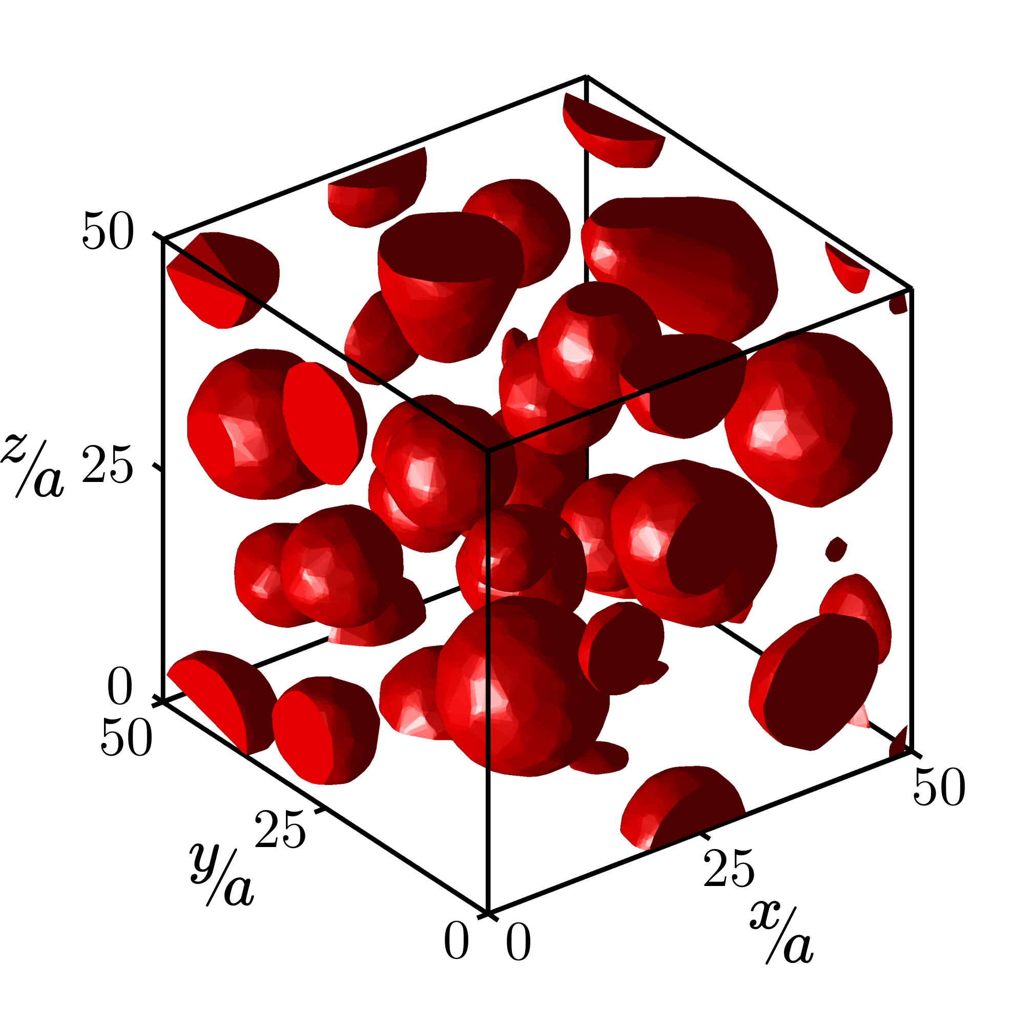
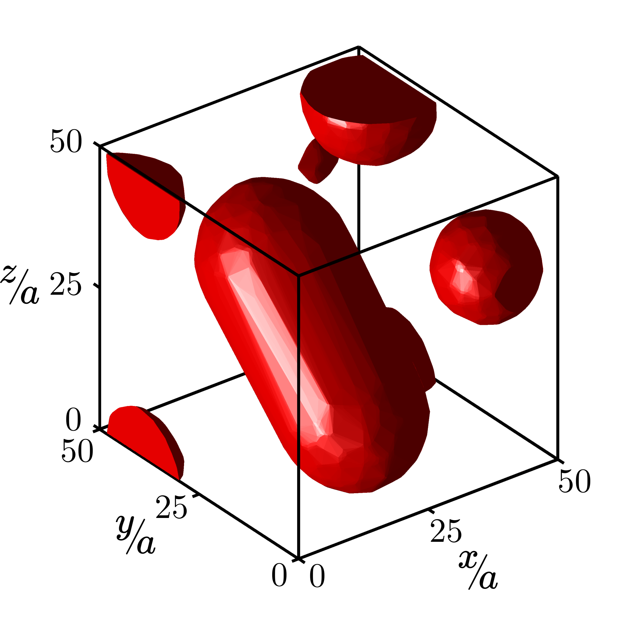
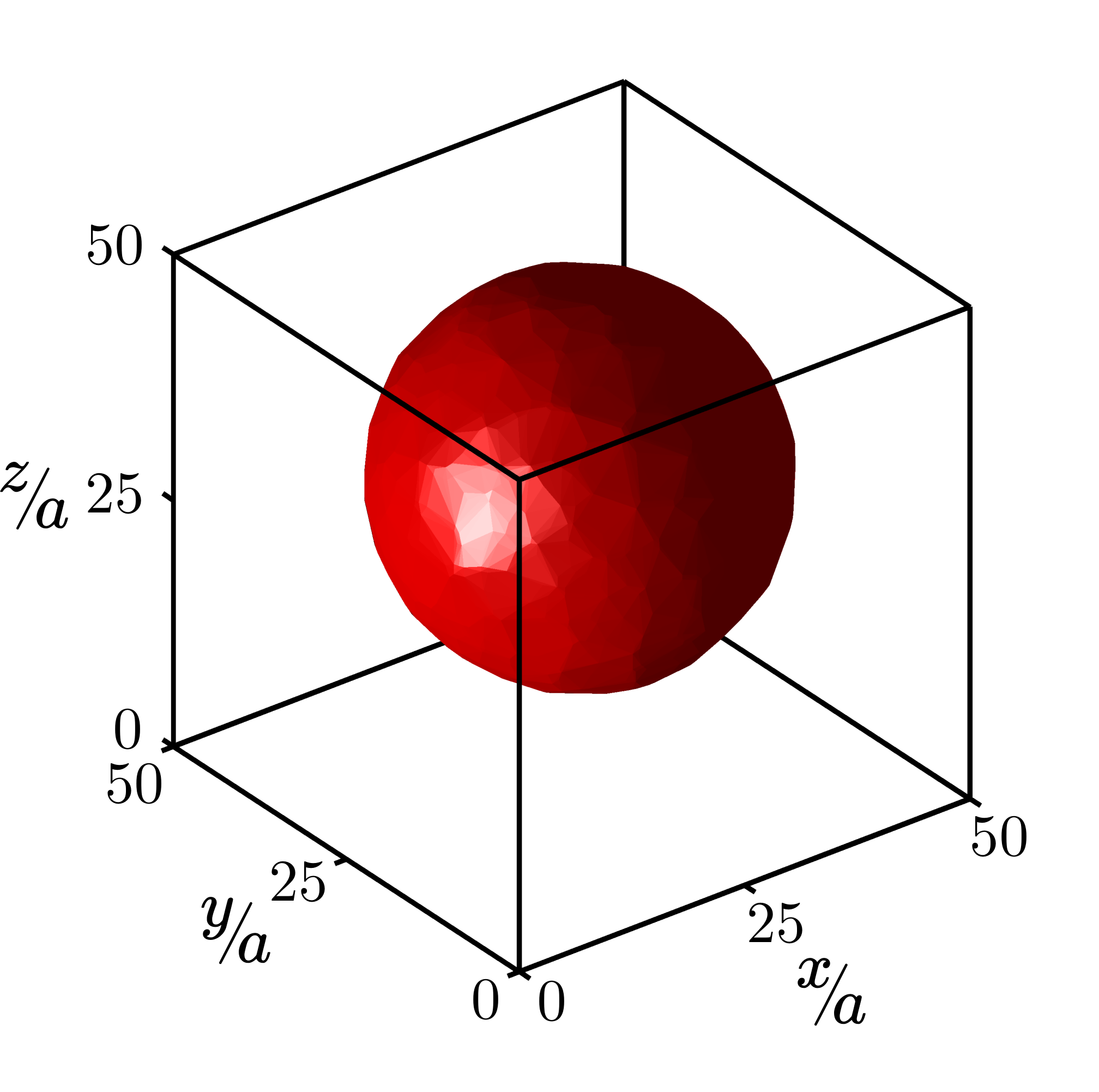
Droplet growth—Ostwald ripening. The generalization of the algorithm to three dimensions is straightforward. To illustrate the time evolution of a phase separating system, we employ the Ginzburg-Landau parameters , , , , and the particle fraction . Similar to the 2D simulations, the actual measured temperature increases slightly by about . Figure 4 presents three snapshots at different simulation times. Initially, the system is totally mixed and evolves to the minimal free-energy conformation. Over time, critical nuclei appear, grow, and coalesce to form larger clusters and droplets. The growth of the clusters is expected to be described by the time evolution of the average radius (Ostwald ripening [29])
| (17) |
where the exponent in the diffusive regime. Figure 5 shows as a function of time. After an initial time, increases approximately in a linear manner. The fit of Eq. (17) yields the exponent , in close agreement with the theoretical value for diffusive growth.
4.1 Interfacial width
In equilibrium, the order-parameter profile of a flat interface in the framework of the Landau theory is given by
| (18) |
where is the bulk order parameter, is the coordinate normal to the interface, and the correlation length characterizes the interfacial width.
To determine the interface profile, we fill the two halfs of the simulation box with and particles, respectively. The Ginzburg-Landau and MPC parameters are chosen to be the same as above (3D system), except is varied from , , to . The obtained stationary state profiles are shown in Fig. 6. Fits to Eq. (18) yield the interfacial widths , , and , whereas Ginzburg-Landau theory predicts , , and . Hence, the simulation values are approximately larger than those predicted by the Ginzburg-Landau theory. This quantitative deviation is not surprising, since the MPC algorithm includes thermal fluctuations, which are not taken into account by the Ginzburg-Landau approach. Indeed, the correlation length increases as at the critical temperature, where in Ginzburg-Landau theory, but for the three-dimensional Ising model. Thus, fluctuations are expected to increase the interface width, in good qualitative agreement with our simulation results. Moreover, the interface widths are on the order of the size of a collision cell, where discretization effects become visible; this makes a detailed quantitative comparison difficult.
5 Conclusions
We have proposed a thermodynamically consistent extension of the MPC algorithm for binary-fluid mixtures, by coupling the Ginzburg-Landau free-energy functional of the density difference between the two fluids to the particle motion in the MPC streaming step. The fluids phase-separate and form, depending on the relative concentration, flat or curved (circle (2D), sphere (3D)) interfaces. The numerical results reproduce the expected capillary-wave spectrum and fulfill the Young-Laplace pressure relation. The analysis of the time dependence of phase separation in 3D, i.e., of the Ostwald-ripening process, proceeds with an exponent , very close to the theoretically expected value (Lifshitz-Slyozov-Wagner growth) in the diffusive regime.
A major advantage of the proposed augmented description of the multicomponent system with an auxiliary order-parameter field is that a broad spectrum of nonlinear fluid equations of state can be implemented easily and conveniently in an otherwise ideal-gas-type fluid. This makes the MPC approach to hydrodynamics applicable to a wide range of phenomena in the dynamics of complex fluids. This approach is particularly useful for studies of synthetic phoretically driven microswimmers, where various kinds of fluids are essential for propulsion [30, 31].
There are various aspects of our novel technique, which deserve further and more detailed study. On the one hand, additional properties of the binary MPC fluid should be addressed, such as transport coefficients or correlation functions. On the other hand, dynamical quantities and critical behavior can be studied. Moreover, extensions are possible to explore the dynamical properties of binary fluids adjacent to walls. Since the free-energy functional of confined systems is available, studies of wetting behavior and contact angles are within reach.
6 Appendix A: Discretization scheme
The fluid velocity obeys the Navier-Stokes equation
| (19) |
Here, the Einstein summation convention over the spatial components , is used. The pressure tensor comprises contributions from the standard MPC algorithm as well as those of the Ginsburg-Landau free-energy functional. The latter contribution can, on the collision cell-level, be equally well written as body-force density acting on the fluid
| (20) |
The change of the velocity due to transport of the immiscible fluids is [20] . Considering particles of type in the discretization volume, i.e., the collision cell, this expression can be written as
| (21) |
We discretize the first term on the RHS of (21) by averaging over two neighbouring cells
| (22) | ||||
which prevents a particle drift.
Here, the force acting on the edges of a collision cell. Hence, when distributing this force onto the particles, the cell as well as neighbouring cells (i.e., or , depending on the Cartesian component) have to be considered.
For the second term in (21), we simply choose a central difference scheme. The discretization scheme for the particles of type differs just by a minus sign in the “bulk” and “interfacal” contributions.
The non-linear pressure contribution is discretized in the same way as the “bulk” term above, with the only difference that no distinction between type or particles has to be made.
Acknowledgements.
We thank A. Wysocki for helpful discussions and suggestions. Support of this work by the DFG priority program SPP 1726 on “Microswimmers – from Single Particle Motion to Collective Behaviour” is gratefully acknowledged.References
- [1] \NameGunstensen A. K., Rothman D. H., Zaleski S. Zanetti G. \REVIEWPhys. Rev A.4319914320.
- [2] \NameShan X. Chen H. \REVIEWPhys. Rev. E4719931815.
- [3] \NameShan X. Chen H. \REVIEWPhys. Rev. E4919942941.
- [4] \NameSwift M. R., Orlandini E., Osborn W. R. Yeomans J. M. \REVIEWPhys. Rev. E5419965041.
- [5] \NameOrlandini E., Swift M. R. Yeomans J. M. \REVIEWEPL (Europhysics Letters)321995463.
- [6] \NameCoveney P. V. Español P. \REVIEWJ. Phys. A301997779.
- [7] \NameKapral R. \REVIEWAdv. Chem. Phys.140200889.
- [8] \NameGompper G., Ihle T., Kroll D. M. Winkler R. G. \REVIEWAdv. Polym. Sci.22120091.
- [9] \NameHashimoto Y., Chen Y. Ohashi H. \REVIEWComput. Phys. Commun.129200056.
- [10] \NameInoue Y., Chen Y. Ohashi H. \REVIEWJ. Comput. Phys.2012004191.
- [11] \NameTüzel E., Pan G., Ihle T. Kroll D. M. \REVIEWEPL80200740010.
- [12] \NameTüzel E., Pan G. Kroll D. M. \REVIEWJ. Chem. Phys.1322010174701.
- [13] \NameHiller T., Sanchez de La Lama M. Brinkmann M. \REVIEWJ. Comput. Phys.3152016554.
- [14] \NameEcheverria C., Tucci K., Alvarez-Llamoza O., Orozco-Guillén E. E., Morales M. Cosenza M. G. \REVIEWFront. Phys.122017128703.
- [15] \NameMalevanets A. Kapral R. \REVIEWJ. Chem. Phys.11019998605.
- [16] \NameHuang C.-C., Gompper G. Winkler R. G. \REVIEWPhys. Rev. E862012056711.
- [17] \NameIhle T. Kroll D. M. \REVIEWPhys. Rev. E632001020201(R).
- [18] \NameHohenberg P. C. Halperin B. I. \REVIEWRev. Mod. Phys.491977435.
- [19] \NameShimizu R. Tanaka H. \REVIEWNat. Commun.620157407.
- [20] \NameTheissen O. Gompper G. \REVIEWEur. Phys. J. B11199991.
- [21] \NameLamura A., Gonnella G. Yeomans J. M. \REVIEWEurophys. Lett.451999314.
- [22] \NameHuang C.-C., Winkler R. G., Sutmann G. Gompper G. \REVIEWMacromolecules43201010107.
- [23] \NameLandau L. D. Lifshitz E. M. \BookStatistical Physics: Vol. 5: Course of Theoretical Physics (Pergamon press, Oxford) 1969.
- [24] \NameReichl L. E. \BookA modern course in statistical physics (John Wiley & Sons, Weinheim) 2016.
- [25] \NameWu F.-Y. \REVIEWRev. Mod. Phys.541982235.
- [26] \NameAnisimov M., Povodyrev A., Kulikov V. Sengers J. \REVIEWPhys. Rev. Lett.7519953146.
- [27] \NameStottrup B. L., Heussler A. M. Bibelnieks T. A. \REVIEWJ. Phys. Chem. B111200711091.
- [28] \NameIhle T., Tüzel E. Kroll D. M. \REVIEWEurophys. Lett.732006664.
- [29] \NameBaldan A. \REVIEWJ. Mater. Sci.3720022171.
- [30] \NameElgeti J., Winkler R. G. Gompper G. \REVIEWRep. Prog. Phys.782015056601.
- [31] \NameBechinger C., Di Leonardo R., Löwen H., Reichhardt C., Volpe G. Volpe G. \REVIEWRev. Mod. Phys.882016045006.