Mori-Zwanzig reduced models for uncertainty quantification
Abstract
In many time-dependent problems of practical interest the parameters and/or initial conditions entering the equations describing the evolution of the various quantities exhibit uncertainty. One way to address the problem of how this uncertainty impacts the solution is to expand the solution using polynomial chaos expansions and obtain a system of differential equations for the evolution of the expansion coefficients. We present an application of the Mori-Zwanzig (MZ) formalism to the problem of constructing reduced models of such systems of differential equations. In particular, we construct reduced models for a subset of the polynomial chaos expansion coefficients that are needed for a full description of the uncertainty caused by uncertain parameters or initial conditions.
Even though the MZ formalism is exact, its straightforward application to the problem of constructing reduced models for estimating uncertainty involves the computation of memory terms whose cost can become prohibitively expensive. For those cases, we present a Markovian reformulation of the MZ formalism which can lead to approximations that can alleviate some of the computational expense while retaining an accuracy advantage over reduced models that discard the memory altogether. Our results support the conclusion that successful reduced models need to include memory effects.
1 Introduction
The problem of quantifying the uncertainty of the solution of systems of partial or ordinary differential equations has become in recent years a rather active area of research. The realization that more often than not, for problems of practical interest, one is not able to determine the parameters, initial conditions, boundary conditions etc. to within high enough accuracy, has led to a flourishing literature of methods for quantifying the impact that this uncertainty imposes on the solution of the problems under investigation (see e.g. [5, 10, 11, 12, 14, 15, 1]). However, despite the increase in computational power and the development of various techniques for uncertainty quantification there is still a wealth of problems where reliable uncertainty quantification is beyond reach. One way to address this problem is to look for reduced models for a subset of the variables needed for a complete description of the uncertainty. The effect of all types of uncertainty is intimately connected with the inherent instabilities that may be present in the underlying system which we subject to the uncertainty. These considerations remain equally, if not more, important when we attempt to construct reduced models for uncertainty quantification.
In the current work, we are concerned with the construction of reduced models for systems of differential equations that arise from polynomial chaos expansions of solutions of a PDE or ODE system. In particular, we focus on the case that the given PDE or ODE system contains uncertain parameters or initial conditions and we want to construct a reduced model for the evolution of a subset of the polynomial chaos expansions that are needed for a complete description of the uncertainty caused by the uncertain parameters. There are different methods to construct reduced models for PDE or ODE systems (see e.g. [6, 4] and references therein). We choose to use the Mori-Zwanzig formalism in order to construct the reduced model [2, 3].
The main issue with all model reduction approaches is the computation of the memory caused by the process of eliminating variables from the given system (referred to as the full system from this point on) [4]. The memory terms are, in general, integral terms which account for the history of the variables that are not resolved. In principle the integrands appearing in the memory terms can be computed through the solution of the orthogonal dynamics equation [3]. We present some examples where this procedure can be implemented and the resulting reduced model can be estimated. Those examples highlight the definite improvement in accuracy of a reduced model when it includes a memory term. However, it is also easy to come up with examples where the solution of the orthogonal dynamics equation becomes prohibitively expensive.
For such cases we present a Markovian reformulation of the MZ formalism which allows the calculation of the memory terms through the solution of ordinary differential equations instead of the computation of convolution integrals as they appear in the original formulation. We present an algorithm which allows the estimation of the necessary parameters on the fly. This means that one starts evolving the full system and use it to estimate the reduced model parameters. Once this is achieved, the simulation continues by evolving only the reduced model with the necessary parameters set equal to their estimated values from the first part of the algorithm. Of course, such an approximation of the memory term cannot work under all circumstances. We present results for a nontrivial problem where it does yield a reduced model with improved behavior compared to a model that ignores the memory terms altogether.
We should note that this alternative approach to computing the memory term fits in the renormalization framework advocated recently by one of the authors [13] in order to construct reduced models for singular PDEs. In particular, the idea is that one embeds the MZ reduced model in a larger family of reduced models which share the same functional form but may have additional parameters for enhanced flexibility. These extra parameters are determined so that the reduced model reproduces some dynamic features of the full system. After this is done, one can switch to the reduced model for the rest of the simulation. In the current work, the extra parameters are the lengths of the memory appearing in the MZ reduced model.
Section 2 presents a brief introduction to the MZ formalism for the construction of reduced models of systems of ODEs. In Section 3 we develop the Markovian reformulation of the MZ formalism and show how one can estimate adaptively the parameters appearing in the reduced model. Section 4 presents numerical results both for the original MZ formalism (Sections 4.1-4.2) and its Markovian reformulation (Section 4.3). Finally, in Section 5 we discuss directions for future work.
2 Mori-Zwanzig formalism
We begin with a brief presentation of the Mori-Zwanzig formalism [2, 3]. Suppose we are given the system
| (1) |
where with initial condition The unknown variables (modes) are divided into two groups, one group is indexed in H and the order indexed in G. Our goal is to construct a reduced model for the modes in the set The system of ordinary differential equations we are given can be transformed into a system of linear partial differential equations
| (2) |
where The solution of (2) is given by . Using semigroup notation we can rewrite (2) as
Suppose that the vector of initial conditions can be divided as where is the vector of the resolved variables (those in ) and is the vector of the unresolved variables (those in ). Let be an orthogonal projection on the space of functions of and
Equation (2) can be rewritten as
| (3) |
where we have used Dyson’s formula
| (4) |
Equation (3) is the Mori-Zwanzig identity. Note that this relation is exact and is an alternative way of writing the original PDE. It is the starting point of our approximations. Of course, we have one such equation for each of the resolved variables . The first term in (3) is usually called Markovian since it depends only on the values of the variables at the current instant, the second is called “noise” and the third “memory”.
If we write
satisfies the equation
| (5) |
If we project (5) we get
since . Also for the initial condition
by the same argument. Thus, the solution of (5) is at all times orthogonal to the range of We call (5) the orthogonal dynamics equation. Since the solutions of the orthogonal dynamics equation remain orthogonal to the range of , we can project the Mori-Zwanzig equation (3) and find
| (6) |
We will not present here more details about how to start from Eq. (6) and construct reduced models of different orders for a general system of ODEs. Such constructions have been documented thoroughly elsewhere (see e.g. [3]). However, we will provide such details for the specific numerical examples in Sections 4.1-4.2.
3 Markovian reformulation of the MZ formalism
While the MZ model given by Eq. (6) is exact, its construction can be involved and most importantly, very costly. The main source of computational expense is the memory term. Technically, the cost associated with the memory term comes from two sources: i) the presence of the orthogonal dynamics equation solution operator and ii) the need to find an expression in terms of the resolved variables and time for which appears in the memory integrand. The presence of is problematic because the orthogonal dynamics equation is, for the general case, a PDE in as many dimensions as the original system of ODEs. Also, finding an expression for is problematic because, in general, it is not possible to separate the dependence of the expression on time and on the resolved variables. Both are formidable tasks and we will show with several examples how they can increase the cost of constructing the reduced model. For some cases (see e.g. Section 4.1 and 4.2) both tasks can be tackled through the use of a finite-rank projection for the operator However, we will show with a simple example (see Section 4.3) that the use of a finite-rank projection may be too costly itself. For such cases, we need an alternative approach to the construction of the memory term. In this section we describe a reformulation of the problem of computing the memory term which can alleviate some of these issues. Also, we present numerical results from the application of this approach in Section 4.3.
3.1 Finite memory
We focus on the case when the memory has a finite extent only. The case of infinite memory is simpler and is a special case of the formulation presented below. Also, the current reformulation allows us to comment on what happens in the case when the memory is very short.
Let by the change of variables Note, that depends both on and the resolved part of the initial conditions We have suppressed the dependence for simplicity of notation. If the memory extends only for units in the past (with ) then
The evolution of is given by
| (7) |
where
To allow for more flexibility, let us assume that the integrand in the formula for contributes only for units with Then
We can proceed and write an equation for the evolution of which reads
| (8) |
where
Similarly, if this integral extends only for units in the past with then
This hierarchy of equations continues indefinitely. Also, we can assume for more flexibility that at every level of the hierarchy we allow the interval of integration for the integral term to extend to fewer or the same units of time than the integral in the previous level. If we keep, say, terms in this hierarchy, the equation for will read
| (9) | |||
where
Note that the last term in (9) involves the unknown evolution operator for the orthogonal dynamics equation. This situation is the well-known closure problem. We can stop the hierarchy at the th term by assuming that
In addition to the closure problem, the unknown evolution operator for the orthogonal dynamics equation appears in the equations for the evolution of the quantities through the various terms respectively.
We describe now a way to express these terms involving the unknown orthogonal dynamics operator through known quantities so that we obtain a closed system for the evolution of
Since we want to treat the case where is not necessarily small, we divide the interval in subintervals. Define
where and Similarly, we can define the quantities
where and In a similar fashion we can define corresponding quantities for all the memory terms up to
In order to proceed we need to make an approximation for the integrals over the subintervals.
3.2 Trapezoidal rule approximation
We have
from which we find
and from (7)
Similarly, for we find
In general,
| (10) |
Similarly,
| (11) |
By dropping the terms we obtain a system of differential equations for the evolution of the quantities This system allows us to determine the memory term Since the approximation we have used for the integral leads to an error the ODE solver should also be We have used the modified Euler method to solve numerically the equations for the reduced model.
Note that the implementation of the above scheme requires the knowledge of the expressions for Since the computation of these expressions for large can be rather involved for nonlinear systems (see Section 4.3), we expect that the above scheme will be used with a small to moderate value of Finally, we mention that the above construction can be carried out for integration rules of higher order e.g. Simpson’s rule.
3.3 Estimation of the memory length
The construction presented above relies on an accurate determination of the memory lengths We present in this section a way to estimate these quantities on the fly. This means that we start evolving the full system, use it to estimate and then switch to the reduced model with the estimated values for
For simplicity of presentation we assume that we evolve only If we use the trapezoidal rule to discretize and eliminate the term from (7), the reduced model reads
| (12) | |||
| (13) |
for We can solve (13) formally and substitute in (12) to get
| (14) |
where Recall that, for the resolved variables, we have from the full system
| (15) |
We would like to estimate the memory decay parameter so that the reduced equation (14) for reproduces the behavior of as predicted by the full system (15). We can do that by requiring that the evolution of some integral quantity of the solution is the same when predicted by the reduced and full systems.
We begin by discretizing the integral term in (14). Suppose that we are evolving the full system with a step size where (note that increases as increases). If we discretize the integral with the trapezoidal rule we find
| (16) | |||
where for The quantities can be computed from the full system.
There is freedom in the choice of the integral quantity whose evolution the reduced model should be able to reproduce. For example, we can use the squared norm of the resolved variables. If we use this integral quantity, then from (16) and (15) we find that the unknown parameter must satisfy
| (17) |
where
and denotes the real part.
Let Then,
| (18) |
With this identification, equation (17) becomes a polynomial equation for with It is not difficult to solve equation (17) with an iterative method, for example Newton’s method. For the numerical results we present in Section 4.3, Newton’s method converged to double precision accuracy within 4-5 iterations. After an estimate has been obtained, we can find the estimate of (recall ) from
| (19) |
3.3.1 Determination of optimal estimate
For each time instant we can obtain through equations (17) and (19), an estimate for Thus, the most important issue that we have to address is that of deciding which is the best estimate of In other words, at what time should we stop estimating the value of so that we can use the estimated value to evolve the reduced model from then on.
We define The quantity monitors the convergence of not only the value of the estimate as a function of the time , but of the whole function Ideally, converges to zero with increasing That will be the case if the approximation of the memory term only through is enough (see (12)-(13)). However, this will not always be the case. If keeping is not enough, then will decrease with increasing up to some time when it will reach a nonzero minimum. After that time, it starts increasing. This signals that keeping only is not enough to describe accurately the memory.
In order to proceed we have two options: (i) construct a higher order model and (ii) identify and thus Results for higher order models will be presented elsewhere (see also discussion in Section 5). In the numerical experiments we present in the next section we have chosen Note that the procedure just outlined allows the automation of the algorithm. This means that there is no adjustable reduced model parameter that needs to be specified at the onset of the algorithm.
We are now in a position to state the adaptive Mori-Zwanzig algorithm which constructs a reduced model with the necessary memory term parameter estimated on the fly.
Adaptive Mori-Zwanzig Algorithm
- 1.
Evolve the full system and compute, at every step, the estimate Use estimates of from successive steps to calculate
- 2.
When reaches a minimum (possibly non zero) value at some instant , pick as the final estimate of
- 3.
For the remaining simulation time (), switch from the full system to the reduced model. The reduced model is evolved with the necessary parameter set to its estimated value
This procedure can be extended to the computation of optimal estimates for i.e. when we evolve, in addition to the quantities Results for such higher order models will be presented elsewhere.
4 Numerical Examples
4.1 A linear ODE with uncertain coefficient
Consider the following linear ordinary equation with an uncertain coefficient
| (20) |
where . This equation has the solution . To represent the dependence of the solution of (20) on we can expand it in a general polynomial chaos (gPC) expansion [16], say using Legendre polynomials. Let , where and are normalized Legendre polynomials which are orthonormal with respect to the uniform distribution of , i.e.,
We can write as . We substitute this expansion in (20) and obtain (through Galerkin projection) the (truncated) system up to order
| (21) |
where and , for (for details, see e.g [17]).
Because of the spectral decay in the gPC coefficients, it is natural to choose the coefficients , of the lower degree Legendre polynomials to be the resolved variables and , to be the unresolved variables respectively. To conform with the notation in Section 2, we have and . We have chosen for the full system and for the reduced system. The solution of the full system is converged for and thus, we do not need to keep further terms in the expansion.
The projection we have chosen is defined as Also, we define To be consistent with the notation in Section 2, we have
In order to be able to compute the expressions for the memory terms we use a finite-rank projection to approximate the projection . To define the finite-rank projection we need to introduce a measure for the distribution of the coefficients. We consider the coefficients to be i.i.d Gaussian random variables with mean at the values given initially (see (21)) and a prescribed variance for In the case of the linear ODE, the variance was set to 0.01 for all the variables in the full system. Also, is the joint probability measure with respect to these random variables. Then for a function of the initial conditions and time, the finite-rank projection reads
| (22) |
where are tensor product Hermite polynomials up to some order , is the multi-index with and is the index set up to order , i.e., . The order for the basis functions was set to 5 for a total of 21 basis functions. In formula (22) the inner product is defined as
| (23) |
For each , the component denotes the solution of the orthogonal dynamics
| (24) |
(24) is equivalent to the Dyson formula:
| (25) |
Eq. (25) is a Volterra integral equation for To proceed, we replace the projection operator with the finite-rank projection operator and find
| (26) |
where
Consequently,
We substitute for in Eq. (25), multiply both sides by and take the inner product with ; the result is (dropping the approximation sign)
| (27) |
Eq. (27) is a Volterra integral equation for the function , which can be rewritten as follows:
| (28) |
where
The functions , can be found by averaging over a collection of experiments or simulations, with initial conditions drawn from the initial distribution. In this example, we use a sparse grid quadrature rule for the multi-dimensional integrals [16].
Finally, we perform one more projection to eliminate the noise term (see Section 2) and the memory term becomes
This can be approximated by
where
After calculating and we obtain the following reduced system,
| (29) |
here and are the matrix form of and , is the initial condition of resolved variables.
Fig. 1 shows the evolution of the memory kernel which is indicative of the behavior of the memory kernels. The basis function is the product of the zero order Hermite polynomial in the variable and the first order Hermite polynomial in the variable We see that the memory kernel is rather slowly decaying which means that the resulting reduced order model will have a long memory. Fig. 2 shows the solution for the resolved variables as predicted by the full system and two different reduced order models, the Markovian model which results from dropping the memory term in (29) and the non-Markovian reduced model given by (29). It is obvious from Fig. 2 that the Markovian model loses accuracy quickly. On the other hand, the non-Markovian model retains its accuracy for the length of the simulation interval. This difference in behavior is quantified in Fig. 3 where we see that for both resolved variables the relative error of the Markovian model becomes greater than by the end of the simulation interval. On the other hand, the error of the non-Markovian model remains less than for the whole simulation interval.


4.2 Nonlinearly damped and randomly forced particle
Consider the following equation describing a particle moving in a double well potential and driven by a force term (see [16])
| (30) |
where and . We use order polynomials in to approximate the full system solution up to time . We want to construct a reduced model for the first 2 coefficients of the polynomial expansion (). As before, we let and we obtain through Galerkin projection the system
| (31) |
where and Let be the vector with . In order to apply the MZ formalism we need an autonomous system of equations to begin with. For this purpose, we introduce an auxiliary time-variable such that and The projection operator projects onto the function space of the first two coefficients and . Again, we use the finite-rank projection onto the function space expanded by Hermite polynomials up to order to represent the orthogonal dynamics (total of 10 functions) and solve the Volterra equation for the memory kernels as we did for the linear ODE example. The variance for the Gaussian variables used to define the inner product for the finite-rank projection was set to for the coefficient with The reason we used a decreasing sequence of variances as we go up in the order of Legendre polynomials is to stabilize the behavior of the reduced model.
As can be seen from Fig. 5, the difference between the (memoryless) Markovian and non-Markovian reduced models is even more pronounced than in the case of the linear ODE. The inclusion of the memory term is indeed crucial for maintaining the accuracy of the reduced model for long times. For the case of the resolved variable the relative error spikes at a couple of points even for the otherwise very accurate non-Markovian reduced model. As can be seen from Fig. 4, this is because the exact value of becomes zero at these points so that the relative error becomes very large even for an accurate approximation. However, the significant improvement in accuracy with the inclusion of the memory term is evident in Fig. 5 which plots the error in a logarithmic scale.


4.3 Viscous 1D Burgers with uncertain initial conditions
In this section we show how the above MZ formulation can be used for uncertainty quantification for the one-dimensional Burgers equation with uncertain initial condition. As is explained at the end of this section, the calculation of the MZ memory term cannot proceed as for the last two examples. The reason is that it is prohibitively expensive due to the number of basis functions needed. Thus, we will apply the alternative construction that was presented in Section 3.
The equation is given by
| (32) |
where Equation (32) should be supplemented with an initial condition and boundary conditions. We solve (32) in the interval with periodic boundary conditions. This allows us to expand the solution in Fourier series
where The equation of motion for the Fourier mode becomes
| (33) |
We assume that the initial condition is uncertain (random) and can be expanded as where is uniformly distributed in and a given function. In the numerical experiments we have taken and Thus, the initial condition varies “uniformly” between the functions 0 and
To proceed we expand the solution for in a polynomial chaos expansion using the standard Legendre polynomials which are orthogonal in the interval In particular, we have that
where is the standard Legendre polynomial of order For each wavenumber we expand the solution of (36) in Legendre polynomials and keep the first polynomials
| (34) |
Similarly, the initial condition can be written as since and Substitution of (34) in (33) and use of the orthogonality property of the Legendre polynomials gives
| (35) |
for and Also
where the expectation is taken with respect to the uniform density on The Legendre polynomial triple product integral defines a tensor which has the following sparsity pattern: if or or or [7]. Due to this sparsity pattern, for a given value of only about of the tensor entries are different from zero.
Before we proceed we have to comment on the cost of applying the MZ formalism to construct a reduced model. We have set the viscosity coefficient to The solution of the full system was computed with Fourier modes () and the first 7 Legendre polynomials (). The first 7 Legendre polynomials were enough to obtain converged statistics for the full system. We want to construct reduced models for the evolution of the coefficients of the first 2 Legendre polynomials i.e., for If we want to apply the MZ formalism in the way we did for the previous two examples (employing a finite-rank projection etc.) we would need to construct a basis in dimensions (exploiting the fact that the solution of the Burgers equation is real-valued). Any attempt to use basis functions up to a high order is infeasible for such a high-dimensional situation. We have attempted to use only low order basis functions but they are not enough to guarantee accuracy of the reduced model. Thus, we turn to the reformulated reduced model that was presented in Section 3.
4.3.1 Reformulated MZ reduced model
To conform with the Mori-Zwanzig formalism we set
where for and Thus, we have
| (36) |
for and We proceed by dividing the variables in resolved and unresolved. In particular, we consider as resolved the variables for and where Similarly, the unresolved variables are for and In the notation of Section 2 we have and In other words, we resolve, for all the Fourier modes, only the first of the Legendre expansion coefficients and we shall construct a reduced model for them.
The system (36) is supplemented by the initial condition We focus on initial conditions where the unresolved Fourier modes are set to zero, i.e. We also define by
To construct a MZ reduced model we need to define a projection operator For a function of all the variables, the projection operator we will use is defined by i.e. it replaces the value of the unresolved variables in any function by zero. Note that this choice of projection is consistent with the initial conditions we have chosen. Also, we define the Markovian term
The Markovian term has the same functional form as the RHS of the full system but is restricted to a sum over only the first Legendre expansion coefficients for each Fourier mode.
For the the term we find
| (37) |
Finally, to implement any method to solve equation (17) for the estimation of we need to specify the RHS of the equation (17). This requires the evaluation of the expression For the case of the viscous Burgers equation, we find
| (38) | |||
Note that since we restrict attention to initial conditions for which the unresolved variables are zero and the projection sets the unresolved variables to zero, the quantity can be computed through the evolution of the full system (36).
The full system was solved with the modified Euler method with The reduced model uses Fourier modes but only the first two Legendre polynomials, so It was solved using the modified Euler method with The parameter needed for the evolution of the memory term was found to be 0.3783 through the procedure described in Section 3.3.1.

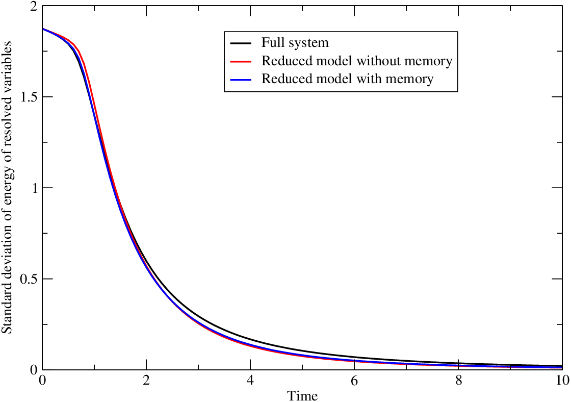
Figure 6 shows the evolution of the mean energy of the solution
as computed from the full system (with Legendre polynomials), the MZ reduced model with without memory (keeping only the Markovian term) and the MZ reduced model with with memory. Figure 7 shows the evolution of the standard deviation of the energy of the solution. The variance of the energy is given by
where
The reduced model performs equally well with or without memory. Of course, the reduced model with memory is slower than the reduced model without memory. However, the reduced model with memory is still about 4 times faster than the the full system.
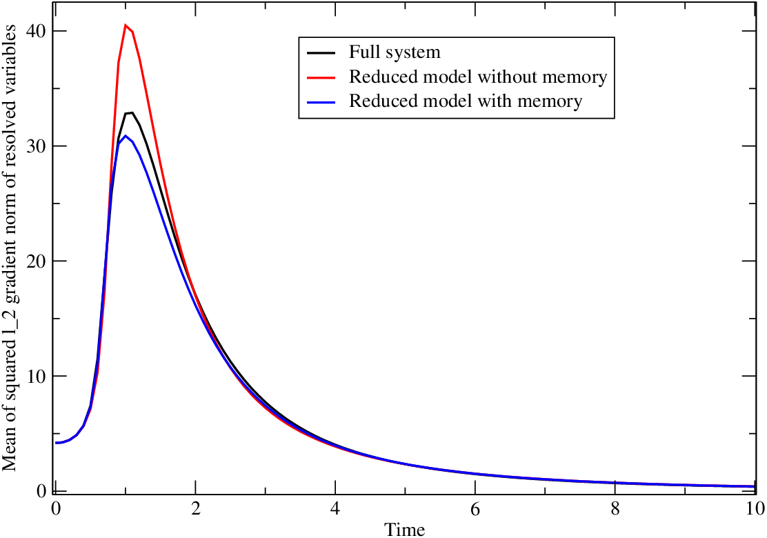
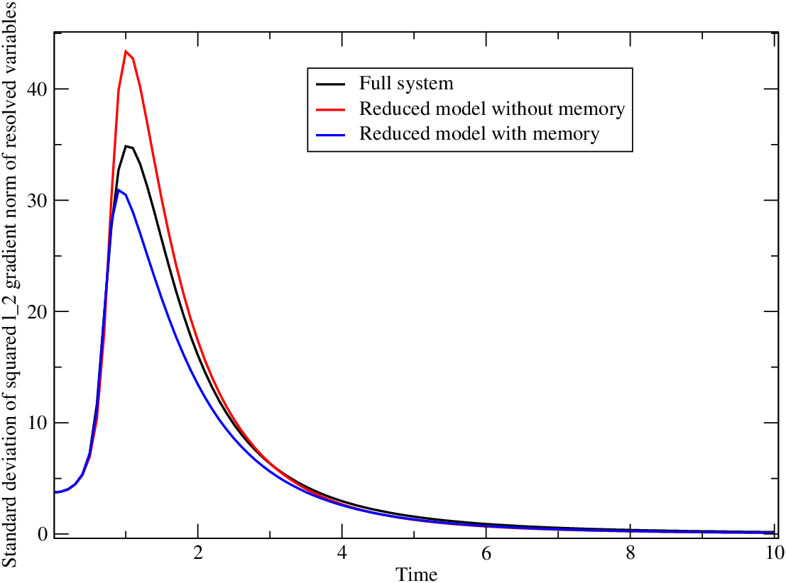
Figure 8 shows the evolution of the mean squared norm of the gradient of the solution
as computed from the full system (with Legendre polynomials), the MZ reduced model with without memory (keeping only the Markovian term) and the MZ reduced model with with memory. Figure 9 shows the evolution of the standard deviation. The variance is given by
The large values of the standard deviation of the mean squared norm of the gradient are justified by the uncertainty in the initial condition. Recall that we have chosen an initial condition which can vary “uniformly” between the functions 0 and As a result, the standard deviation is large because it has to account for a wide range of possible initial conditions.
It is evident from the figures that the inclusion of the memory term improves the performance of the reduced model. Also, it is evident that there is room for improvement of the reduced model with memory. In particular, more terms are needed in the reformulated MZ model to approximate better the memory.
Recall that the solution of Burgers equation is a contraction [9]. Eventually, the complete description of the uncertainty caused by the uncertainty in the initial condition requires only a few polynomial chaos expansion coefficients. This happens at a time scale that is dictated by the magnitude of the viscosity coefficient. That is why for long times the reduced model with and without memory have comparable behavior to that of the full system. However, for short times, the inclusion of the memory term does make a difference because information from the higher chaos expansion coefficients is needed. The higher chaos expansion coefficients will have a more prolonged contribution for systems that possess unstable modes. In such cases, the inclusion of the memory term becomes imperative for short as well long times. Results for such cases will be presented elsewhere.
5 Discussion and future work
We have examined the application of the Mori-Zwanzig formalism to the problem of constructing reduced models for uncertainty quantification. In particular, we have constructed reduced models for subsets of the polynomial chaos expansion coefficients needed to describe fully the uncertainty. We have examined cases of parametric or initial condition uncertainty. The main conclusion from the current work is that while the MZ formalism can be applied for the construction of reduced models, the task of constructing an efficient (or even feasible) reduced model can be involved. For cases where the straightforward application of the MZ formalism is not possible, we have offered an alternative construction. The implementation of this alternative construction is reminiscent of renormalization constructions used to describe the evolution of complex solutions of PDEs [13].
The current work opens several directions for future work. First, we should investigate whether there is a more economical way of choosing the basis functions for cases when the basis functions have many arguments (as was the case for the Burgers example). This is important because the calculation of the memory kernels through the finite-rank projection is well defined and the solution of the corresponding Volterra equations can be performed with high accuracy. A related question is whether there is sparsity in the coefficients of the basis functions. It is plausible that even though in principle the number of basis functions to reach a specific order may be very large, many of them may not contribute to the representation. A related approach would be the use of machine learning algorithms to obtain a more efficient representation of the memory term. Finally, a related issue to be investigated is how to ensure the stability of the reduced model when the finite-rank projection is employed. For example, for the nonlinearly damped and forced particle case, we had to assign smaller variances for the higher coefficients to stabilize the reduced model. This procedure needs to be investigated and, if possible, automated.
A second interesting research direction has to do with the representation of the memory term when the finite-rank projection is not possible due to a prohibitively large number of basis functions. We have explored here an expansion of the memory term that involves, in essence, a Taylor expansion of the orthogonal dynamics operator. Such an expansion seems more plausible when the timescale of the orthogonal dynamics is slower than that of the resolved variables. However, there is an alternative way of performing the expansion of the memory term that is more suited to the case when the orthogonal dynamics is faster than the resolved variables. Such an expansion leads to a Taylor expansion of the whole memory term, not just the orthogonal dynamics operator. If the memory kernel becomes insignificant after a time interval then one can use the full system up to time estimate the Taylor expansion of the whole memory term around time and then switch to the reduced model with the memory given by the Taylor expansion. We will investigate this alternative memory representation and report the results elsewhere.
6 Acknowledgements
The authors would like to thank D. Barajas-Solano, H. Lei and A. Tartakovsky for useful discussions and comments. This research at Pacific Northwest National Laboratory (PNNL) was partially supported by the U.S. Department of Energy (DOE) Office of Advanced Scientific Computing Research (ASCR) Collaboratory on Mathematics for Mesoscopic Modeling of Materials (CM4), under Award Number DE-SC0009280 and partially by the U.S. DOE ASCR project “Uncertainty Quantification For Complex Systems Described by Stochastic Partial Differential Equations”. PNNL is operated by Battelle for the DOE under Contract DE-AC05-76RL01830.
References
- [1] Barajas-Solano D.A. and Tartakovsky A.M., Probabilistic density function method for nonlinear dynamical systems driven by colored noise, Phys. Rev. E 93(5) (2016) DOI:10.1103/PhysRevE.93.052121.
- [2] Chorin, A.J., Hald, O.H. and Kupferman, R., Optimal prediction and the Mori-Zwanzig representation of irreversible processes, Proc. Nat. Acad. Sci. USA 97 (2000) pp. 2968-2973.
- [3] Chorin, A.J., Hald, O.H. and Kupferman, R., Optimal prediction with memory, Physica D 166 (2002) pp. 239-257.
- [4] Chorin, A.J. and Stinis, P., Problem reduction, renormalization and memory, Comm. App. Math. Comp. Sci. 1 (2005) pp. 1-27.
- [5] Ghanem R. and Spanos P.D., Stochastic finite elements: a spectral approach, Springer-Verlag, 1998.
- [6] Givon, D., Kupferman, R. and Stuart, A., Extracting macroscopic dynamics: model problems and algorithms, Nonlinearity 17 (2004) pp. R55-R127.
- [7] Gupta M. and Narasimhan S.G., Legendre polynomials Triple Product Integral and lower-degree approximation of polynomials using Chebyshev polynomials, Technical Report - CMU-RI-TR-07-22, Carnegie Mellon, 2007.
- [8] Hou T.Y., Luo W., Rozovskii B. and Zhou H.M., Wiener Chaos Expansions and Numerical Solutions of Randomly Forced Equations of Fluid Mechanics, J. Comput. Phys. 216 (2006) pp. 687-706.
- [9] Lax P.D., Hyperbolic Systems of Conservation Laws and the Mathematical Theory of Shock Waves, SIAM Publications, Philadelphia, 1972.
- [10] Leonenko G. and Phillips T., On the solution of the Fokker-Planck equation using a high-order reduced basis approximation, Comput. Methods Appl. Mech. Engrg., 199(1-4) (2009) pp. 158-168.
- [11] Ma X. and Zabaras N., An adaptive hierarchical sparse grid collocation method for the solution of stochastic differential equations, J. Comput. Phys., 228 (2009) pp. 3084-3113.
- [12] Nouy A. and Le Maître O. P., Generalized spectral decomposition for stochastic nonlinear problems, J. Comput. Phys., 228 (2009) pp. 202-235.
- [13] Stinis P., Renormalized reduced models for singular PDEs, Communications in Applied Mathematics and Computational Science Vol. 8 (2013), No. 1, pp. 39-66.
- [14] Venturi D., A fully symmetric nonlinear biorthogonal decomposition theory for random fields, Physica D, 240(4-5) (2011) pp. 415-425.
- [15] Wan X. and Karniadakis G. E., Multi-element generalized polynomial chaos for arbitrary probability measures, SIAM J. Sci. Comput., 28(3) (2006) pp. 901-928.
- [16] Xiu D. and Hesthaven J.S., High-Order Collocation Methods for Differential Equations with Random Inputs, SIAM J. Sci. Comput. 27(3), pp. 1118-1139.
- [17] Xiu D. and Karniadakis G.E., The Wiener–Askey Polynomial Chaos for Stochastic Differential Equations, SIAM J. Sci. Comput., 24(2) (2002), pp. 619-644.