De Broglie relations, gravitational time dilation and weak equivalence principle

Quantum theory and general relativity both reveal the unusual properties of the physical world that depart from our everyday experiences and intuitions. Interplays between them had long inspired theoretical investigations and exciting studies of new phenomena. For example, a quantum theory of gravity that sees the consistent merger of these two fundamental theories [1] has been a long-sought goal in theoretical physics. Novel predictions, such as black hole radiations [2, 3, 4], had been drawn from the studies of quantum fields in curved spacetime [5]. Ideas of gravitational decoherence [6], first suggested by Diósi [7, 8] and Penrose [9, 10], had also shed some new light on the quantum measurement problem. Recently, gravitational time dilation in quantum interferometry have been studied in a series of works [11, 12, 13, 14], and their relations with the equivalence principle has brought up active discussions [15, 16, 17, 18, 19, 20].

Besides those advances from combining quantum theory and gravitation, there lies subtle connections and consistencies between these two seemingly different perspectives of the physical world. An important example of such consistencies is the uniqueness of free-falling or inertial motions in both quantum and gravitational physics, which may relate the nature of quantum fluctuations to gravitation [21, 22, 23]. As summarized by Smolin in [21], that having quantum fluctuations, inertia and gravitation being the absolutely universal phenomena, the preferred motions singled out by vanishing the dissipation effects from quantum fluctuations (spectrum properties of vacuum quantum fluctuations) are exactly the free-falling or inertia motions considered in classical general relativity. In the hydrodynamic formulation of quantum mechanics first proposed by Madelung [24], the evolutions of the probability density and current of a quantum system are governed by the Madelung equations which contain a quantum potential quadratic in the Planck’s constant. The Madelung equations had then provided the basis for different classical interpretations of quantum mechanics including the stochastic interpretation due to Nelson [25, 26]. The uniqueness of inertial motions is also manifested in the stochastic interpretation of quantum mechanics, that the diffusion constant or the correlation length of the particle subjected to quantum fluctuations is inversely proportional to a quantity with the dimension of mass [26, 23], and the equivalence of such “quantum mass” and the inertia mass ensures the linearity of the (Schrödinger type) equation that is governing the evolution of the probability density and current of the particle subjected to quantum fluctuations [21, 22, 23]. Such agreements between these two seemingly unrelated fields may not be taken merely as a coincidence, but could possibly be “the central mystery behind the question of the relationship between quantum and gravitational phenomena” as pointed out by Smolin [21]. In this work, we try to re-investigate such connections through the unique properties of free-falling or inertial motions. The key result turns out to be that, if in curved spacetime the clock rate differences or gravitational time dilations in different parts of a quantum system are taken into account, the universality of inertial or free-falling (mean) motions of quantum test particles or bodies in gravitational field may naturally be deduced from the fundamental de Broglie relations. This leads to a novel perspective that the classical weak equivalence principle (WEP) may be deeply rooted in quantum physics and be a phenomenon that has emerged from the quantum world. In deriving this, after introducing the framework in the next section, we consider a quantum scalar wave packet propagated in a classical weakly curved spacetime background, and, except for the de Broglie relations, no assumption of priori given Hamiltonians or least actions satisfied by the quantum wave is made.

The principle of equivalence is the foundation of the geometric view of gravitation. Summarized in the 1964 Les Houches lecture given by Dicke [27], the Einstein equivalence principle (EEP) contains three ingredients: WEP, Lorentz invariance and position independence of non-gravitational physical laws in local free-falling frames. WEP states that trajectories of free-falling test particles or bodies in gravitational fields are independent of their internal structures and compositions. In the history of the developments of gravitational theories, from the opening pages of Newton’s Principia to Einstein’s gedanken experiment of a free-falling elevator, WEP had played a crucial role. Connections between WEP and the other two ingredients of EEP are believed to exist, and the Schiff’s conjecture, see [28], states that any complete and self-consistent theory of gravity that embodies WEP will necessarily embody the full EEP. Given the full EEP, it can be further argued that gravitation must be the phenomena of curved spacetime and satisfy the so called metric theories [27]. WEP, or the universality of free-fall, is therefore at the very heart of modern theories of gravitation.

If the fundamental notion of curved spacetime is accepted, in metric theories (including general relativity as the best fit candidate confronted with the many stringent tests [28, 29]), WEP is fulfilled due to one basic postulate that matter fields couple to gravity in a universal manner. For test masses, this means that free-falling motions follow the shortest paths (geodesic lines) in curved spacetime endowed with a symmetric metric tensor field $g_{\mu\nu}$ (the indices $\mu,\nu=0,1,2,3$). Such postulate also imposes absolute structures to these geometric theories of gravitation, such as the non-dynamical and priori given coupling constants, see [27, 30, 28] for detailed discussions. This had firstly been questioned since 1930s by Dirac and Jordan [31, 32, 33], which leads to a perspective that WEP may be only an approximation valid in the low energy realm of gravity [30, 28]. On the other hand, attempts to construct a full quantum formulation of WEP are also under the research, see [34, 35] and the references therein. Today, precision tests (including quantum tests [36, 37]) of WEP and EEP, considered as an approach to discover new physics, are of interest, and the most updated result from MICROSCOPE has set the upper bound of the Eötvös-ratio to be about $10^{-15}$ [38]. In the following, we try to tackle this issue from a different angle.

To manifest the potential interweaving between spacetime geometry and quantum laws, one needs a stage for the low-energy realm which could bring these two together under common considerations. In the following, we assume that the velocity $v$ of the test mass (classical or quantum) is much smaller compared with the speed of light, and the gravitational field generated by the test mass itself could be ignored. Units system $c=G=\hbar=1$ is adopted for clarity. The quantum state of a test particle or a macroscopic quantum system (such as superfluids) is considered as a square integrable complex wave function $\Psi(t,\vec{x})$ distributed over a certain spacetime region. For clarity, spins and other internal degrees of freedom are not considered in this work. In the low-energy regime, we assume that the gravitational field or the spacetime curvature is weak in the sense that the scale $L$ of the wave function $\Psi(t,\vec{x})$ (such as the characteristic width of Gaussian wave packets) is much smaller compared with the curvature radius $\mathcal{R}$ in that spacetime region, that $L/\mathcal{R}\ll$1. Therefore, it is natural to choose Fermi normal coordinate systems [39] $\{t,\ x^{i}\}$ as reference frames, within which the spacetime metric components could be expanded in powers of $\mathcal{O}(\frac{|x|}{\mathcal{R}})$ with $|x|/\mathcal{R}\ll 1$. In a general Riemann manifold, the Fermi normal coordinates system generalized the classical Riemann normal coordinates (that satisfies the conditions $g_{\mu\nu}(0)=\eta_{\mu\nu}$ and $\Gamma_{\ \mu\nu}^{\lambda}(0)=0$) with the connection coefficients $\Gamma_{\ \mu\nu}^{\lambda}$ vanished along a given curve. With such curve being chosen as a time-like geodesic, the Fermi normal coordinates system can be physically viewed as the local frame attached to the observer following that geodesic, and its local tetrad is formed by the clock and parallel transported rigid rods carried by the observer. Up to $\mathcal{O}(\frac{|x|^{2}}{\mathcal{R}^{2}})$, the spacetime metric under the Fermi normal frame can be expanded as [40, 41]

	$\displaystyle ds^{2}$	$\displaystyle=$	$\displaystyle-(1+R_{0i0j}x^{i}x^{j})dt^{2}-(\frac{4}{3}R_{0jik}x^{j}x^{k})dtdx^{i}$		(1)
			$\displaystyle+(\delta_{ij}-\frac{1}{3}R_{ikjl}x^{k}x^{l})dx^{i}dx^{j},$

where $t$ is the proper time measured by the observer centered at the origin and $R_{\mu\nu\lambda\rho}\sim\frac{1}{\mathcal{R}^{2}}$ is the Riemann curvature tensor evaluated along the observer’s world line. Einstein summation convention is adopted.

As mentioned, for test masses in metric theories (including general relativity), to embody WEP or the universality of free-falling motions, a separate postulate of shortest paths (least action) is needed

$$S=\mu\int\sqrt{-g_{\mu\nu}\frac{dx^{\mu}}{dt}\frac{dx^{\nu}}{dt}}dt=\mu\int d\tau,$$

(2)

where $\tau$ is the proper time experienced by the test mass $\mu$. With the low energy conditions $v^{i}=\frac{dx^{i}}{dt}\ll 1$, $\frac{d\tau}{dt}\sim 1$, the metric component $g_{00}$ in the above action weights the most in evaluating the length of the world line, and therefore affects the motion mostly. Given the metric expansion in Eq. (1), the equation of free-falling or geodesic motions from the above action can be cast into the simple and linearized form in local Fermi normal frames [40, 41]

$$a^{i}=\frac{d^{2}x^{i}}{dt^{2}}=-R_{0j0i}x^{j}+\mathcal{O}(\frac{|x|v}{\mathcal{R}^{2}}),$$

(3)

here $R_{0i0j}$ can be viewed as a symmetric matrix (the tidal matrix) with indices $i,j=1,2,3$. As expected, this equation of motion is independent of the internal structures and compositions of the classical test particles or bodies, and therefore manifests the fulfillment of WEP that viewed from the local frame of a free observer.

Within the local Fermi normal frame as the common stage, the classical model of test mass $\mu$ is replaced with the corresponding quantum wave packet $\Psi(t,\vec{x})$ (usually a Gaussian wave packet), whose characteristic scale $L$ is much smaller compared with the curvature radius $\mathcal{R}$ in the local frame. According to Eq. (1), the metric is then expanded in terms of the components of the curvature tensor about a flat background. Without loss of generality, the wave packet can be expanded in terms of Fourier modes

$$\Psi(t,\vec{x})=\frac{1}{(2\pi)^{\frac{3}{2}}}\int A(\vec{k})e^{-i\left(\omega(k)t-\vec{k}\cdot\vec{x}\right)}d^{3}k.$$

(4)

Normally, how does such quantum system respond to or interact with spacetime curvatures could be answered by assuming a specific action (or a Hamiltonian) that coupled to the gravitational field [42, 5], as for the case of classical test particles or bodies. Generally, different choices may yield different dynamical equations. For example, for the scalar wave $\Psi(t,\vec{x})$ considered here, the minimal coupling may be a preferred choice since with this choice the strong version of equivalence principle could be fulfilled. Here we discard such priori given actions, and try to derive the preferred mean motions of quantum test masses driven by the fundamental de Broglie relations.

According to de Broglie relations, the total energy $\mathcal{E}$ and momentum $\vec{p}$ of the quantum system $\Psi(t,\vec{x})$ are associate to its frequency $\omega$ and wave vector $\vec{k}$. Therefore, in the low energy limit that $p\ll\mu$, an overall phase term can be factored out

$$\Psi(t,\vec{x})=e^{-2\pi i\mu t}\psi(t,\vec{x}),$$

(5)

where, according to Eq. (4), one has

$$\psi(t,\vec{x})=\frac{1}{(2\pi)^{\frac{3}{2}}}\int A(\vec{k})e^{-i(\frac{k^{2}}{4\pi\mu}t-\vec{k}\cdot\vec{x})}d^{3}k.$$

This is because for each Fourier mode one has $\omega(k)/2\pi=\mathcal{E}(k)=\mu+\frac{k^{2}}{(2\pi){}^{2}2\mu}+...$ with the characteristic or mean momentum $<p>=<k/2\pi>\ \ll\mu$. This is a well-known result in non-relativistic quantum mechanics, and usually the overall phase factor $e^{-2\pi i\mu t}$ is ignored since it is expected to have no measurable effect in the low-energy regime. But, concerning the universality of the free-falling motions in curved spacetime, such phase factor from the rest mass $\mu$ will play an important part in restoring the classical free-falling motions (given in Eq. (3)) or the classical WEP that is viewed in local frames.

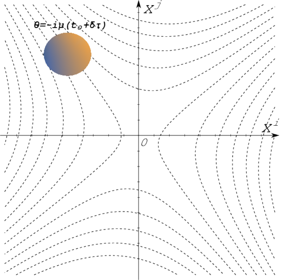
Let us take the atomic clocks [43, 44] in gravitational red shift experiments [28, 45] and Bose-Einstein condensates in free-falling experiments [37] as typical examples concerning quantum systems in gravitational fields, compared to the curvature radius the corresponding quantum systems or wave packets are viewed as being sharply peaked at or bounded to some small space regions. It is assumed that such quantum systems are evolved according to the proper time of the co-moving frame attached to the mass center of the experimental platform. While, this is still of an averaged or approximated treatment. In [11, 12, 13, 14], such treatment is generalized for the case that the propagation of a quantum system is in superpositions of different paths in gravitational fields that are having different proper time dilations. In this work, with one step forward, we suggest that with a natural generalization more detailed behaviors of an extensively distributed quantum wave could be studied. According to the classical free-falling motions in the low-energy and weak field limit, we notice from Eq. (1) - (3) that the test mass probes the variations and non-uniformities of the metric component $g_{00}$ much stronger than those of other components, since the test mass follows slowly (compared to the speed of light) along a time-like worldline in the reference frame. The metric component $g_{00}$ can be viewed as a measurement of the non-uniformity of the time flows or clock rates at different points in the local Fermi normal frame, see Fig. 1 for an illustration. This naturally inspired us that, for an extensive test body or system (quantum or classical) moving slowly compared with the speed of light in gravitational field, the time parameter of each part or at each point of the system should be counted as the proper time $\tau$ measured by the clock located in that part or at that point. In fact, for classical extensive bodies such clock rate differences just give rise to the tidal forces subjected to them from spacetime curvature, if the priori given least action of matter fields coupled to gravity is imposed. While, given the de Broglie relations which indicate the associations between 4-momenta and spacetime periodic patterns, an important difference between quantum and classical systems is that the phase at different part of a quantum system is strongly correlated. Therefore, without any priori given action, such differences of the clock rates $d\tau/dt$ in the different parts of a quantum wave packet $\Psi(\tau,\vec{x})$ in curved spacetime are expected to generate additional phase variations and will drive the motions of the quantum test system.

Without loss of generality, let us start with a space slice at $t=t_{0}$ in the local Fermi frame. After the coordinate time lapse $\delta t=t-t_{0}$, which is the proper time lapse recorded by the observer centered at the origin, the proper time lapse experienced at point $x^{i}$ will be

	$\displaystyle\delta\tau$	$\displaystyle=$	$\displaystyle\sqrt{1+R_{0i0j}x^{i}x^{j}+\mathcal{O}(\frac{|x|^{2}v}{\mathcal{R}})}\delta t$		(6)
		$\displaystyle=$	$\displaystyle\left(1+\frac{1}{2}R_{0i0j}x^{i}x^{j}+\mathcal{O}(\frac{|x|^{2}v}{\mathcal{R}})\right)\delta t,$

see again Fig. 1 for an illustration. Therefore, the clock rate at point $x^{i}$ with respect to the observer’s proper time reads

$$\frac{\delta\tau}{\delta t}=1+\frac{1}{2}R_{0i0j}x^{i}x^{j}+\mathcal{O}(\frac{|x|^{2}v}{\mathcal{R}}).$$

For the wave function $\Psi(\tau,\vec{x})$ distributed over the space slice, such clock rate differences over the corresponding space region will generate additional phase differences among the different parts of $\Psi(\tau,\vec{x})$ and then result in a variation in the corresponding wave vector.

In the space slice $t=t_{0}$, one denotes the wave function as $\Psi(t_{0},\vec{x})=e^{-2\pi i\mu t_{0}}\psi(t_{0},\vec{x})$ with a uniform initial phase $2\pi\mu t_{0}$ in the overall phase factor from the rest mass $\mu$, and the possible initial non-uniformity in the phase is left in the $\psi(t_{0},\vec{x})$ part, see Fig. 2a for illustration.

After the coordinate time lapse $\delta t=t-t_{0}$, the wave function becomes $\Psi(t_{0},\vec{x})\rightarrow\Psi(t_{0}+\delta\tau,\vec{x})$ with $\delta\tau$ given in Eq. (6), that

			$\displaystyle\Psi(t_{0}+\delta\tau,\vec{x})$		(7)
		$\displaystyle=$	$\displaystyle e^{-2\pi i\mu(t_{0}+\delta\tau)}\psi(t_{0}+\delta\tau,\vec{x})$
		$\displaystyle=$	$\displaystyle e^{-2\pi i\mu\left(\frac{1}{2}R_{0i0j}x^{i}x^{j}+\mathcal{O}(\frac{|x|^{2}v}{\mathcal{R}})\right)\delta t}e^{-i\mu(t_{0}+\delta t)}\psi(t_{0}+\delta\tau,\vec{x}),$
		$\displaystyle=$	$\displaystyle e^{-\pi i\mu R_{0i0j}x^{i}x^{j}\delta t}\Psi(t,\vec{x}).$

Therefore we have $\Psi(t_{0},\vec{x})\rightarrow e^{-\pi i\mu R_{0i0j}x^{i}x^{j}\delta t}\Psi(t,\vec{x})$, where $\Psi(t,\vec{x})$ is obtained by time shifting the free wave $\Psi(t_{0},\vec{x})$ with the common coordinate lapse $\delta t$

$$\Psi(t,\vec{x})=e^{-2\pi i\mu t}\frac{1}{(2\pi)^{\frac{3}{2}}}\int A(\vec{k})e^{-i(\frac{k^{2}}{4\pi\mu}t-\vec{k}\cdot\vec{x})}d^{3}k.$$

For the last equal in Eq. (7), we make use of the low-energy condition $\mu\gg\ <p>=<k>/2\pi$ and ignore the higher order terms of $\mathcal{O}(\frac{<k>^{2}}{\mu^{2}})\mathcal{O}(\frac{|x|^{2}}{\mathcal{R}}\mu)$ in the phase. This could be made more clear when one considers the Fourier expansions given in Eq. (4)

			$\displaystyle\Psi(t_{0}+\delta\tau,\vec{x})$
		$\displaystyle=$	$\displaystyle e^{-2\pi i\mu\left(\frac{1}{2}R_{0i0j}x^{i}x^{j}+\mathcal{O}(\frac{|x|^{2}v}{\mathcal{R}})\right)\delta t}e^{-2\pi i\mu(t_{0}+\delta t)}\frac{1}{(2\pi)^{\frac{3}{2}}}\int A(\vec{k})e^{-i\left[\frac{k^{2}}{4\pi\mu}\left(t_{0}+[1+\frac{1}{2}R_{0i0j}x^{i}x^{j}+\mathcal{O}(\frac{|x|^{2}v}{\mathcal{R}})]\delta t\right)-\vec{k}\cdot\vec{x}\right]}d^{3}k$
		$\displaystyle=$	$\displaystyle e^{-2\pi i\mu\left(\frac{1}{2}R_{0i0j}x^{i}x^{j}+\mathcal{O}(\frac{|x|^{2}v}{\mathcal{R}})\right)\delta t}e^{-2\pi i\mu(t_{0}+\delta t)}\frac{1}{(2\pi)^{\frac{3}{2}}}\int A(\vec{k})e^{-i\left(\frac{k^{2}}{4\pi\mu}(t_{0}+\delta t)-\vec{k}\cdot\vec{x}\right)-i\mathcal{O}(\frac{k^{2}}{\mu^{2}})\mathcal{O}(\frac{|x|^{2}}{\mathcal{R}}\mu)\delta t}d^{3}k$
		$\displaystyle=$	$\displaystyle e^{-\pi i\mu R_{0i0j}x^{i}x^{j}\delta t}\Psi(t,\vec{x}).$

Therefore, evolved to the subsequent space slice $t=t_{0}+\delta t$, the clock rate differences in the weakly curved spacetime produce a phase difference $\delta\theta=-\pi\mu R_{0i0j}x^{i}x^{j}\delta t$ in the wave function, see Fig. 2b for an illustration. Between two adjacent points $x^{i}$ and $x^{i}+\Delta x^{i}$ in the quantum wave packet, such phase difference reads

$$\Delta(\delta\theta)=-2\pi\mu R_{0i0j}x^{i}\Delta x^{j}\delta t,$$

(8)

Phase variations are modulated to $2\pi$, therefore the above phase difference accumulated during $\delta t$ over the space interval $\Delta\vec{x}$ will be wrapped into a ripple with the wave length $2\pi\Delta x/\Delta(\delta\theta)$, see Fig. 2c for an illustration, and then results in a variation in the wave vector $\delta\vec{k}$ after $\delta t$

$$\delta k_{i}=\frac{\Delta(\delta\theta)}{\Delta x^{i}}=-2\pi\mu R_{0j0i}x^{j}\delta t.$$

(9)

Now, according to the de Broglie relations $p_{i}=k_{i}/2\pi$, the variations in wave vector imply the variations in the momenta $\delta p_{i}=\mu\delta v^{i}$, therefore the mean value of the velocity variations or the acceleration of the quantum test mass can be obtained as

	$\displaystyle<\frac{\delta v^{i}}{\delta t}>$	$\displaystyle=$	$\displaystyle<\frac{\delta k_{i}}{2\pi\mu\delta t}>$
	$\displaystyle<a^{i}>$	$\displaystyle=$	$\displaystyle-R_{0j0i}<x^{j}>.$		(10)

This gives rise to the expected semi-classical version of the free-falling or geodesic equation in gravitational fields viewed in local Fermi normal frames, which is independent of the mass and composition of the quantum test system and will restore Eq. (3) as one takes the classical limits. Therefore, within the low energy regime, the classical WEP could be restored from such universality of quantum mean motions in gravitational fields.

In the following, we give a more straightforward derivation of Eq. (10). Given the de Broglie relations, the velocity density takes the form

$$v^{i}=\frac{p_{i}}{\mu}=-\frac{i}{4\pi\mu}(\Psi^{*}\nabla_{i}\Psi-\Psi\nabla_{i}\Psi^{*}).$$

According to the Fourier expansions of the quantum wave in Eq. (4) and (7), for the initial slice $t=t_{0}$ the mean velocity of the quantum test mass reads

			$\displaystyle<v^{i}(t_{0})>$
		$\displaystyle=$	$\displaystyle\int-\frac{i}{2\mu}\left(\Psi^{*}(t_{0},\vec{x})\nabla_{i}\Psi(t_{0},\vec{x})-\Psi(t_{0},\vec{x})\nabla_{i}\Psi^{*}(t_{0},\vec{x})\right)d^{3}x$
		$\displaystyle=$	$\displaystyle\frac{1}{2\pi\mu}\int|A(\vec{k})|^{2}k_{i}d^{3}k$
		$\displaystyle=$	$\displaystyle\frac{<k^{i}>}{2\pi\mu},$

and, as evolved to the subsequent slice $t=t_{0}+\delta t$, one has

			$\displaystyle<v^{i}(t_{0}+\delta t)>$
		$\displaystyle=$	$\displaystyle\int-\frac{i}{2\mu}[e^{\pi i\mu R_{0i0j}x^{i}x^{j}\delta t}\Psi^{*}(t,\vec{x})\nabla_{i}\left(e^{-\pi i\mu R_{0i0j}x^{i}x^{j}\delta t}\Psi(t,\vec{x})\right)$
			$\displaystyle-e^{-\pi i\mu R_{0i0j}x^{i}x^{j}\delta t}\Psi(t,\vec{x})\nabla_{i}\left(e^{\pi i\mu R_{0i0j}x^{i}x^{j}\delta t}\Psi^{*}(t,\vec{x})\right)]d^{3}x$
		$\displaystyle=$	$\displaystyle\frac{1}{2\pi\mu}\int|A(\vec{k})|^{2}k_{i}d^{3}k-R_{0k0i}\delta t\int\psi^{*}(t,\vec{x})x^{k}\psi(t,\vec{x})d^{3}x$
		$\displaystyle=$	$\displaystyle\frac{<k_{i}>}{2\pi\mu}-R_{0j0i}<x^{j}>\delta t$
			$\displaystyle+\mathcal{O}(\frac{<x><v>}{\mathcal{R}}\mu)\delta t+\mathcal{O}(\frac{<k>^{2}}{\mu^{2}})\mathcal{O}(\frac{<x>}{\mathcal{R}}\mu)\delta t.$

With the increment in the mean velocity after $\delta t$

	$\displaystyle<\delta v^{i}>$	$\displaystyle=$	$\displaystyle<v^{i}(t_{0}+\delta t)>-<v^{i}(t_{0})>$		(11)
		$\displaystyle=$	$\displaystyle-R_{0j0i}<x^{j}>\delta t$
			$\displaystyle+\mathcal{O}(\frac{<x><v>}{\mathcal{R}}\mu)\delta t+\mathcal{O}(\frac{<k>^{2}}{\mu^{2}})\mathcal{O}(\frac{<x>}{\mathcal{R}}\mu)\delta t,$

we have

	$\displaystyle<a^{i}>$	$\displaystyle=$	$\displaystyle\frac{<\delta v^{i}>}{\delta t}$		(12)
		$\displaystyle=$	$\displaystyle-R_{0k0i}<x^{k}>$
			$\displaystyle+\mathcal{O}(\frac{<x><v>}{\mathcal{R}}\mu)+\mathcal{O}(\frac{<k>^{2}}{\mu^{2}})\mathcal{O}(\frac{<x>}{\mathcal{R}}\mu),$

which restores the expected semi-classical equation (10). One notices that this derivation applies to general wave functions $\Psi(t,\vec{x})$, and the resulting mean values (the first moments) $<\delta v^{i}>$ and $<a^{i}>$ do not depend on the structures or “shapes” of the quantum wave packets.

Within the low-energy realm, if one takes into account the clock rate differences or gravitational time dilations in the different parts of a test quantum wave packet that is distributed over a weakly curved spacetime, the de Broglie relations for the correlated phase in the quantum wave will naturally drive the mean motions of the quantum test system to follow the classical free-falling trajectories. The mean velocity variation given in Eq. (11) or the mean acceleration in Eq. (12) in weak gravitational fields does not depend on the masses or compositions of the quantum test systems or the shapes of the corresponding quantum waves. Such mean motions of free quantum test systems in gravitational fields agree exactly with the classical free-falling or geodesic motions given in Eq. (3), which are determined by the background geometries. Therefore, as one takes the classical limit, such universality of quantum mean motions implies the WEP in the macroscopic world. Remember again that the classical free-falling or geodesic equation in geometric (metric) theories of gravitation is obtained by an additional postulate of shortest paths for test masses or a universal coupling of matter fields to gravity, while here the quantum equation does not rely on any such priori given action or Hamiltonian but can be deduced naturally with the aids of the de Broglie relations. This reveals, in a new angle, the connections between the fundamental quantum laws and the general notion of curved spacetime, and also a possible link between the de Broglie relations and WEP. More interestingly, this also suggests a novel perspective that WEP, as the foundation of gravitational theories, could be deeply rooted in quantum physics and be emerged from the quantum world.

Only mean motions of test quantum wave packets are considered here. Quantum fluctuations beyond the mean motions that are affected by weakly curved spacetime can be studied in terms of variances, covariances and higher moments within this formalism. For wave packets that deviate largely from a sharply peaked Gaussian packet (classical limits) or are Gaussian packets with highly asymmetric shapes, whether or not quantum fluctuations affected or caused by spacetime curvatures could produce measurable effects is of interest and worthy of further investigations. At last, we have made use of Fermi normal frames for the low-energy weak-field regime and the linearized classical geodesic equation to bring together the quantum and gravitational effects to interweave with each other. To further reinforce the central idea, extensions to more general cases, especially with internal degrees of freedom such as spins and couplings to strong gravitational fields, could be addressed.

Acknowledgments.— The authors thank Yao Cheng from Tsianghua University and Yun Kau Lau from Chinese Academy of Sciences for the valuable suggestions and discussions. The NSFC Grands No. 11571342, National Key R&D Program of China No.2017YFC0602202 and Natural Science Basic Research Plan in Shaanxi Province of China No. 2017JQ1028 are acknowledged. The authors are also supported by the State Key Laboratory of Scientific and Engineering Computing, Chinese Academy of Sciences.

References

- [1] Kiefer, C. Quantum Gravity (Oxford University Press, Oxford, 2012), third edn.
- [2] Hawking, S. W. Particle creation by black holes. Communications In Mathematical Physics 43, 199–220 (1975). URL http://link.springer.com/10.1007/BF02345020.
- [3] Hawking, S. W. Black holes and thermodynamics. Physical Review D 13, 191–197 (1976). URL https://link.aps.org/doi/10.1103/PhysRevD.13.191.
- [4] Wald, R. M. The Thermodynamics of Black Holes. Living Reviews in Relativity 4, 6 (2001). URL http://link.springer.com/10.12942/lrr-2001-6.
- [5] Wald, R. M. Quantum Field Theory in Curved Spacetime and Black Hole Thermodynamics (The University of Chicago Press, Chicago and London, 1994).
- [6] Bassi, A., Großardt, A. & Ulbricht, H. Gravitational decoherence. Classical and Quantum Gravity 34, 193002 (2017). URL https://link.aps.org/doi/10.1103/PhysRevD.68.085006.
- [7] Diósi, L. Gravitation and quantum-mechanical localization of macro-objects. Physics Letters A 105, 199–202 (1984). URL http://linkinghub.elsevier.com/retrieve/pii/0375960184903979.
- [8] Diósi, L. Models for universal reduction of macroscopic quantum fluctuations. Physical Review A 40, 1165–1174 (1989). URL https://link.aps.org/doi/10.1103/PhysRevA.40.1165.
- [9] Penrose, R. On Gravity’s role in Quantum State Reduction. General Relativity and Gravitation 28, 581–600 (1996). URL http://link.springer.com/10.1007/BF02105068.
- [10] Penrose, R. On the Gravitization of Quantum Mechanics 1: Quantum State Reduction. Foundations of Physics 44, 557–575 (2014). URL http://link.springer.com/10.1007/s10701-013-9770-0.
- [11] Zych, M., Costa, F., Pikovski, I. & Brukner, Č. Quantum interferometric visibility as a witness of general relativistic proper time. Nature Communications 2, 505 (2011). URL http://www.nature.com/doifinder/10.1038/ncomms1498.
- [12] Zych, M., Costa, F., Pikovski, I., Ralph, T. C. & Brukner, Č. General relativistic effects in quantum interference of photons. Classical and Quantum Gravity 29, 224010 (2012). URL http://iopscience.iop.org/article/10.1088/0264-9381/29/22/224010/meta.
- [13] Pikovski, I., Zych, M., Costa, F. & Brukner, Č. Universal decoherence due to gravitational time dilation. Nature Physics 11, 668–672 (2015). URL http://www.nature.com/doifinder/10.1038/nphys3366.
- [14] Pikovski, I., Zych, M., Costa, F. & Brukner, Č. Time dilation in quantum systems and decoherence. New Journal of Physics 19, 025011 (2017). URL http://iopscience.iop.org/article/10.1088/1367-2630/aa5d92/meta.
- [15] Bonder, Y., Okon, E., & Sudarsky, D. Can gravity account for the emergence of classicality?. Physical Review D 92, 124050 (2015). URL https://journals.aps.org/prd/abstract/10.1103/PhysRevD.92.124050
- [16] Adler, S. L., & Bassi, A. Gravitational decoherence for mesoscopic systems. Physics Letters A 380, 390-393 (2016). URL https://www.sciencedirect.com/science/article/pii/S0375960115009561
- [17] Bonder, Y., Okon, E., & Sudarsky, D. Questioning universal decoherence due to gravitational time dilation. Nature Physics 12, 2 (2016). URL https://www.nature.com/articles/nphys3573
- [18] Pikovski. I., Zych, M., Costa, F., & Brukner, Č. Reply to ’Questioning universal decoherence due to gravitational time dilation’. Nature Physics 12, 2-3 (2016). URL https://www.nature.com/articles/nphys3650
- [19] Pang, B. H., Chen, Y. & Khalili, F. Y. Universal Decoherence under Gravity: A Perspective through the Equivalence Principle. Physical Review Letters 117, 090401 (2016). URL https://journals.aps.org/prl/abstract/10.1103/PhysRevLett.117.090401.
- [20] Diósi, L. Centre of mass decoherence due to time dilation: paradoxical frame-dependence. Journal of Physics: Conference Series 880, 012020 (2017). URL https://iopscience.iop.org/1742-6596/880/1/012020/
- [21] Smolin, L. On the nature of quantum fluctuations and their relation to gravitation and the principle of inertia. Classical and Quantum Gravity 3, 347–359 (1986). URL http://iopscience.iop.org/article/10.1088/0264-9381/3/3/009/meta.
- [22] Smolin, L. Quantum gravity and the statistical interpretation of quantum mechanics. International Journal of Theoretical Physics 25, 215–238 (1986). URL http://link.springer.com/10.1007/BF00668705.
- [23] Smolin, L. Quantum fluctuations and inertia. Physics Letters A 113, 408–412 (1986). URL http://linkinghub.elsevier.com/retrieve/pii/0375960186906614.
- [24] Madelung, E. Quantentheorie in hydrodynamischer Form. Zeitschrift für Physik 40, 322 (1926). URL https://link.springer.com/article/10.1007%2FBF01400372?LI=true.
- [25] Nelson, E. Derivation of the Schrödinger Equation from Newtonian Mechanics. Physical Review 150, 1079–1085 (1966). URL https://link.aps.org/doi/10.1103/PhysRev.150.1079.
- [26] Nelson, E. Dynamical theories of brownian motion (Princeton University Press, 1967).
- [27] Dicke, R. H. Experimental relativity. In DeWitt, C. & DeWitt, B. (eds.) Relativity, Groups and Topology, 165–316 (Gordon and Breach, 1964).
- [28] Will, C. M. The Confrontation between General Relativity and Experiment. Living Reviews in Relativity 17, 1–113 (2014). URL http://www.livingreviews.org/lrr-2014-4.
- [29] Ni, W.-T. Solar-system tests of the relativistic gravity. International Journal of Modern Physics D 25, 1630003 (2016). URL http://www.worldscientific.com/doi/abs/10.1142/S0218271816300032.
- [30] Damour, T. Theoretical aspects of the equivalence principle. Classical and Quantum Gravity 29, 184001 (2012). URL http://iopscience.iop.org/article/10.1088/0264-9381/29/18/184001/meta.
- [31] DIRAC, P. A. M. The Cosmological Constants. Nature 139, 323–323 (1937). URL http://www.nature.com/articles/139323a0.
- [32] Jordan, P. Die physikalischen Weltkonstanten. Die Naturwissenschaften 25, 513–517 (1937). URL http://link.springer.com/10.1007/BF01498368.
- [33] Jordan, P. Über die kosmologische Konstanz der Feinstrukturkonstanten. Zeitschrift für Physik 113, 660–662 (1939). URL https://link.springer.com/article/10.1007/BF01340095.
- [34] Zych, M., & Brukner, C. Quantum Formulation of the Einstein Equivalence Principle. Nature Physics 14,1027-1031 (2018). URL https://www.nature.com/articles/s41567-018-0197-6.
- [35] Anastopoulos, C. & Hu, B. L. Equivalence principle for quantum systems: dephasing and phase shift of free-falling particles. Classical and Quantum Gravity 35, 035011 (2018). URL http://iopscience.iop.org/article/10.1088/1361-6382/aaa0e8/meta.
- [36] Viola, L. & Onofrio, R. Testing the equivalence principle through freely falling quantum objects. Physical Review D 55, 455-462 (1997). URL https://journals.aps.org/prd/abstract/10.1103/PhysRevD.55.455.
- [37] van Zoest, T. et al. Bose-Einstein Condensation in Microgravity. Science 328, 1540–1543 (2010). URL http://www.sciencemag.org/cgi/doi/10.1126/science.1189164.
- [38] Touboul, P. et al. MICROSCOPE Mission: First Results of a Space Test of the Equivalence Principle. Physical Review Letters 119, 231101 (2017). URL https://link.aps.org/doi/10.1103/PhysRevLett.119.231101.
- [39] Nesterov, A. I. Riemann normal coordinates, Fermi reference system and the geodesic deviation equation. Classical and Quantum Gravity 16, 465–477 (1999). URL http://iopscience.iop.org/article/10.1088/0264-9381/16/2/011/meta.
- [40] Misner, C. W., Thorne, K. S. & Wheeler, J. A. GRAVITATION (W. H. Freeman, San Francisco, 1973).
- [41] Ni, W.-T. & Zimmermann, M. Inertial and gravitational effects in the proper reference frame of an accelerated, rotating observer. Physical Review D 17, 1473–1476 (1978). URL https://link.aps.org/doi/10.1103/PhysRevD.17.1473.
- [42] Birrell, N. D. & Davies, P. C. W. Quantum Fields in Curved Space (Cambridge University Press, Cambridge, 1984).
- [43] Cacciapuoti, L. & Salomon, C. Space clocks and fundamental tests: The ACES experiment. The European Physical Journal Special Topics 172, 57–68 (2009). URL http://www.springerlink.com/index/10.1140/epjst/e2009-01041-7.
- [44] Lévèque, T. et al. PHARAO laser source flight model: Design and performances. Review of Scientific Instruments 86, 033104 (2015). URL http://aip.scitation.org/doi/10.1063/1.4914025.
- [45] Jetzer, P. General relativity tests with space clocks in highly elliptic orbits. International Journal of Modern Physics D 26, 1741014 (2017). URL http://www.worldscientific.com/doi/abs/10.1142/S0218271817410140.