Babenko’s equation for periodic gravity waves on water of finite depth: derivation and numerical solution

The classical formulation proposed by Benjamin and Lighthill is convenient for justification of their conjecture (see [36] and [37], where it had been justified for Stokes waves and all near-critical waves respectively). In this formulation, $Q$ — the constant rate of flow per channel’s unit span — is prescribed along with the total head $R$ also referred to as the Bernoulli constant. Let Cartesian coordinates $(X,Y)$ be chosen so that the bottom coincides with the $X$-axis and gravity acts in the negative $Y$-direction, whereas the wave profile has a crest on the $Y$-axis (this does not restrict generality). Thus, the profile is given by the graph of an unknown positive function $\xi$ (that is, $Y=\xi(X)$, $X\in\mathbb{R}$), attaining its maximum at $X=0$. Moreover, we suppose that $\xi$ is continuously differentiable and even. In the longitudinal section of the water domain ${\cal D}=\{X\in\mathbb{R},\ 0<Y<\xi(X)\}$, the velocity field is described by the stream function $\Psi(X,Y)$, that is, the projections of the velocity vector at $(X,Y)$ on the $X$- and $Y$-axis are $\Psi_{Y}$ and $-\Psi_{X}$ respectively. It is assumed that $\Psi$ belongs to $C^{2}({\cal D})\cap C^{1}(\bar{\cal D})$ and is an even function of $X$ (hence it is bounded on $\bar{\cal D}$).

If the surface tension is neglected, then $\Psi$ and $\xi$ must satisfy the following free-boundary problem:

In the left-hand side of the last relation usually referred to as Bernoulli’s equation, $g>0$ is the constant acceleration due to gravity. It is known that non-trivial solutions of problem (3)–(6) exist only when $Q\neq 0$ and $R>R_{c}=\frac{3}{2}(Qg)^{2/3}$. For the proof of the first relation see Proposition 1.1 in [38], whereas the last inequality is proved in [39] under weaker assumptions than listed above. In what follows, these restrictions on $Q$ and $R$ hold; moreover, we suppose (without loss of generality) that $Q>0$.

Let us assume that $\xi$ is a $2\ell$-periodic function ($\ell>0$), whereas $\Psi(X,Y)$ is $2\ell$-periodic in $X$, but the constant $R$ is to be found along with these functions from problem (3)–(6). In order to reduce the reformulated problem to a non-dimensional form, we average Bernoulli’s equation over $(-\ell,\ell)$. Since $\Psi$ is constant on the free surface, we obtain that $c^{2}=2(R-gH)$, where

Here $n$ is the unit normal to $Y=\xi(X)$ directed out of ${\cal D}$. One can show that the last equality (7) is true with the same constant $c^{2}$ when this curve is changed to $Y=\tilde{\xi}(X)$ — an arbitrary streamline — and $n$ is changed to $\tilde{n}$ — the unit normal to this streamline. Therefore, $c>0$ is the unknown mean velocity of flow in the positive direction of the $X$-axis.

It is convenient to introduce the following non-dimensional quantities: $h=\pi H/\ell$ (the mean depth of flow) and $Q_{0}=Q/\sqrt{g(\ell/\pi)^{3}}$ (the rate of flow). Now we scale the dimensional variables and shift the vertical variables downwards as follows:

This is advantageous because the new unknown $\eta$ is a $2\pi$-periodic and even function of $x$ satisfying the following condition:

Furthermore, the function $\psi$ has the same properties on $\bar{D}$ as $\Psi$ has on $\bar{\cal D}$; namely,

and is a $2\pi$-periodic and even function of $x$. Moreover, the change of variables (8) reduces relations (3)–(6) to the following

In the non-dimensional Bernoulli equation, the parameter $\mu=\pi c^{2}/(g\ell)$ is the Froude number squared which must be found along with $\eta$ and $\psi$. Besides, $\mu/2$ serves as the independent of $h$ upper bound for $\eta$ with equality achieved only for the wave of extreme form with the Lipschitz crest; see [32]. Thus, the non-dimensional statement of the problem is as follows.

On the other hand, having a solution of problem P$(Q_{0},h)$, formulae (8) yield a $2\ell$-periodic solution of problem (3)–(6) for any $\ell>0$, for which purpose one has to put $Q=Q_{0}\sqrt{g(\ell/\pi)^{3}}$ and to determine $R$ from the equality $c^{2}=2(R-gH)$ with $c^{2}=\mu g\ell/\pi$ and $H=h\ell/\pi$.

First, we follow considerations in Section 8 of [9]; see also the rather recent paper [40]. By $w(z)=\varphi+\kern 0.50003pt\mathrm{i}\kern 0.50003pt\psi$ $(z=x+\kern 0.50003pt\mathrm{i}\kern 0.50003pty)$ we denote the complex potential restricted to the one-wave domain $D_{2\pi}=\{-\pi<x<\pi,-h<y<\eta(x)\}$ of some periodic wave on water of a certain depth $h$. Here $\varphi(x,y)$ is the odd in $x$ harmonic conjugate to $\psi$, for which purpose the additive constant must be chosen properly. For some $r\in(0,1)$ we consider a conformal mapping, say $u(z)$, from the $z$-plane to the auxiliary $u$-plane; it maps $D_{2\pi}$ onto

This annular domain has a cut which makes it simply connected and the map is such that the images of the upper and bottom parts of $\partial D_{2\pi}$ are

respectively, whereas the left (right) side of $\partial D_{2\pi}$ is mapped onto the upper (lower respectively) side of the cut $\{\Re\,u\in(-1,-r)\ \mbox{when}\ \Im\,u=0\}$. Putting

where $f(u)$ is a certain Laurent series, one obtains that

In [9], Section 8, this formula serves as the basis for deriving Nekrasov’s equation in the case of finite depth. An equivalent form of this equation is given in [40]; see equation (1.1) there.

According to the second equality (15), the general form of the inverse conformal mapping $A_{r}\ni u\mapsto z\in D_{2\pi}$ is as follows:

Here, we put minus at $a_{0}$ because it is convenient in what follows. The fact that all coefficients $a_{k}$ are real is a consequence of equality (16) because $\psi$ is equal to a real constant on the bottom part of $\partial D_{2\pi}$ which corresponds to $\{|u|=r;\Re\,u\neq-r\}$ — the circumference cut on the negative real axis.

Let us derive some relations for the coefficients from (17). First, for $u=r$ we obtain

Substituting $u=\textrm{e}^{\kern 0.40974pt\mathrm{i}\kern 0.40974ptt}$, $t\in(-\pi,\pi)$, into (17) and separating the real and imaginary parts, we arrive at the following parametric representation of the free surface profile:

Now we see that another relation is equivalent to condition (9) written in terms of the last two expressions, namely:

It follows from the last equality that $a_{0}>0$ in the non-trivial case. Then equality (18) shows that the value of $r$ is related not only to the depth $h$, but also to a particular solution of problem P$(Q_{0},h)$.

It is worth mentioning that both expressions (19) are similar to those for the infinite depth (cf. [21], Section 3.7, where Babenko’s results are outlined), and in that case, a consequence is the relation $x_{t}=-1-\mathcal{C}\eta_{t}$ with

which is the form of the $2\pi$-periodic Hilbert transform alternative to formulae (2).

The crucial point for obtaining a similar relation in the case of finite depth is to introduce the operator $\mathcal{B}_{r}=\mathcal{C}+\mathcal{K}_{r}$ for $r\in(0,1)$, where

It is straightforward to calculate that $\mathcal{B}_{r}$ can also be defined on $L^{2}(-\pi,\pi)$ by linearity from the following relations

that are similar to (2). Combining these formulae and (19) yields that

An important fact about the operator $\mathcal{B}_{r}$ is that it is a conjugation in the following sense. If $F(u)$ is analytic in $A_{r}$ and $\Im F$ vanishes identically on $\{|u|=r;\Re\,u\neq-r\}$, then

Let us calculate the derivative $z_{\varphi}$ of the mapping inverse to the complex potential. In view of the first equality (15), we have

Combining this and (17), we obtain that

and the function on the right-hand side is analytic in $A_{r}$. Since $z_{\varphi}$ does not vanish in the closure of $A_{r}$, we have that $z_{\varphi}^{-1}=|\nabla\varphi|^{2}\,\overline{z_{\varphi}}$ is also analytic in $A_{r}$. Moreover, the Bernoulli equation (13) implies that

(cf. formula (3.38) in [21]). Here the second equality is a consequence of the Cauchy–Riemann equations. Then equality (23) yields that

It follows from previous considerations that the constant in the Laurent expansion of $z_{\varphi}^{-1}$ is equal to $\mu$. Furthermore, $\Im\{z_{\varphi}^{-1}-\mu\}$ vanishes identically on $\{|u|=r;\Re\,u\neq-r\}$, which allows us to apply formula (24) to the function $z_{\varphi}^{-1}-\mu$, whose trace on $\{u=\textrm{e}^{\kern 0.40974pt\mathrm{i}\kern 0.40974ptt}\}$ is equal to

Here again ^′ stands for differentiation with respect to $t$. Thus, we arrive at

which simplifies to Babenko’s equation for waves on water of finite depth:

This equation is similar to (1) and the derivation procedure yields that for each $r\in(0,1)$ it is related to some solution of problem P$(Q_{0},h)$.

To show the existence of small solutions of equation (28), bifurcating from the zero solution, we apply the Crandall–Rabinowitz theorem (see [41], Theorem 1.7) that deals with bifurcation from simple eigenvalues of the linearised equation; its formulation is as follows.

As in [19], we say that a real-valued function $v$ belongs to the Sobolev space $H_{0}$ provided it is absolutely continuous on $[-\pi,\pi]$, $v(-\pi)=v(\pi)$, and its weak derivative $v^{\prime}$ belongs to $L^{2}(-\pi,\pi)$. Let $\hat{H}_{0}$ be the subspace of $H_{0}$ consisting of even functions.

In terms of the map ${\cal F}:\mathbb{R}\times\hat{H}_{0}\mapsto L^{2}(-\pi,\pi)$ defined by

equation (28) takes the following form:

Let us apply the Crandall–Rabinowitz theorem to this equation to obtain local branches of Stokes-wave solutions of small amplitude, for which purpose we have to check conditions (i)–(iv) for ${\cal F}(\mu,v)$.

It is clear that (i) and (ii) are fulfilled and ${\cal F}_{v}(\mu,0)=\mu\mathcal{B}_{r}\,(\mathrm{d}\kern 0.2pt/\mathrm{d}\kern 0.2ptt)-I$, where $I$ is the identity operator. Hence the set of bifurcation points of equation (30) is $\{\mu_{n}\}_{n=1}^{\infty}$, where

are the characteristic values of $\mathcal{B}_{r}\,(\mathrm{d}\kern 0.2pt/\mathrm{d}\kern 0.2ptt)$. Furthermore, ${\cal F}_{v}(\mu_{n},0)$ is a Fredholm operator, its index is equal to zero for every $\mu_{n}$, and the corresponding null-space in $\hat{H}_{0}$ is one-dimensional being generated by $v^{(0)}_{n}(t)=\cos nt$, thus yielding condition (iii). Since ${\cal F}_{\mu v}(\mu_{n},0)=-I$ we see that ${\cal F}_{\mu v}(\mu_{n},0)v^{(0)}_{n}(t)=-\cos nt$, and so condition (iv) for $n=1,2,\dots$ is a consequence of the fact that the equation

has no solution. Indeed, a solution of this equation exists if and only if its right-hand side is orthogonal to the null-space of the adjoint operator

Since its null-space is one-dimensional and generated by $\cos nt$, the orthogonality condition does not hold for $-\cos nt$. This completes verification of condition (iv).

Then the Crandall–Rabinowitz theorem yields the following.

The last assertion is a consequence of the fact that ${\cal F}_{vv}$ is continuous which is obvious. This theorem is illustrated in Fig. 1, where we have a plot of the bifurcation branch $C_{1}$ in terms of $\mu$ and the norm of solution $\|v\|_{\infty}$ in the space $L^{\infty}(-\pi,\pi)$. The plotted branch bifurcating from $\mu_{1}(4/5)$ has no secondary bifurcation points as the analogous branch for equation (1); see [19, 20] for the rigorous proof and detailed discussion. Moreover, it exhibits the phenomenon of a turning point at the largest value of $\mu$ attained on $C_{1}$, occurring high on the branch; see further details in Section 4.3. (The fastest traveling wave of given period corresponds to this point.) By means of a different method this property was demonstrated by [32], whereas our method shows that it also takes place for equation (1) on the branch bifurcating from $\mu_{1}(0)$. This phenomenon is related to the ‘Tanaka instability’ found numerically in [42], and later investigated analytically in [43].

Let us outline a procedure demonstrating how to obtain a solution of problem (10)–(13) from that of Babenko’s equation; that is, if equation (28) with $r\in(0,1)$ is satisfied by some $\mu>0$ and an even function $v$ (the existence of such pairs — at least in the form (32) — follows from Theorem 2), then one can find the following:

(1) a $2\,\pi$-periodic, symmetric curve with zero mean and a negative number $-h$, which define the wave profile and the level of horizontal bottom, respectively, thus giving a one-period water domain, say $\Omega$, on the $(x,y)$-plane;

(2) a function $\psi$ harmonic in $\Omega$ and vanishing on its top side and two positive constants serving as the right-hand side terms in the boundary conditions (11) and (13).

Let we have an even, $2\pi$-periodic solution $v$ of equation (28), whose Fourier coefficients we denote $b_{0},b_{1},b_{2},\dots$ to distinguish these coefficients from those in (17), and let the periodic extension of $v$ to $\mathbb{R}$ be real-analytic. Using these coefficients, we define the following holomorphic function on $A_{r}$:

Here $B$ is a real number that will be determined below in terms of the Fourier coefficients of $v$. Let us consider the images that correspond under this mapping to the curves and segments of $\partial A_{r}$. First, we see that $z(\textrm{e}^{\kern 0.40974pt\mathrm{i}\kern 0.40974ptt})=x(t)+\kern 0.50003pt\mathrm{i}\kern 0.50003pty(t)$ for $t\in(-\pi,\pi)$, where

Since this curve given parametrically serves as the upper part of $\partial\Omega$, we require its mean value to vanish. This gives that

where the series converges because the Fourier coefficients of the real-analytic $v$ decay faster than any power of $k$.

Now we are in a position to determine the mean depth of flow $h$. In view of symmetry we have that $z(r)$ is the mid-point of the bottom; that is, $z(r)=-\kern 0.50003pt\mathrm{i}\kern 0.50003pth$. Then putting $u=r$ into (33), we find that

and so is positive; here the last equality is a consequence of (35). Thus, the second expression (34) takes the following form:

Hence the curve $z_{s}=\{x=x(t)=-t-(\mathcal{B}_{r}\,y)(t),\ \ y=y(t);\ \ t\in[-\pi,\pi]\}$ has the zero mean value. Here, the first formula (22) is applied to express $x(t)$ in terms of $y(t)$.

Furthermore, we have

thus obtaining two vertical segments $z_{-}$ and $z_{+}$ on the lines $x=-\pi$ and $x=\pi$ respectively.

Taking into account (35) and (36), we see that

on the inner circumference. This defines a horizontal segment $z_{b}$ on the line $y=-h$.

It is clear that the curve $\Gamma=z_{+}\cup z_{s}\cup z_{-}\cup z_{b}$ constructed above is closed and one can check (for example, numerically) that the set $\Omega$ enclosed within $\Gamma$ is a domain. The next step is to show that $z(u)$ defined with the help of the Fourier coefficients of $v$ is a conformal mapping of $A_{r}$ onto $\Omega$. For this purpose one can use the boundary correspondence principle; its form relevant for our case (see, for example, [44], Chapter 5, Theorem 1.3) is formulated for the convenience of the reader.

According to this theorem $z(u)$ maps $A_{r}$ onto $\Omega$ conformally provided one can show (for example, numerically) that the map $\partial A_{r}\ni u\mapsto z\in\Gamma$ is a homeomorphism. Moreover, condition (9) is fulfilled for $\eta(x)=y(t(x))$; here $t(x)$ is the inverse of $x=-t-(\mathcal{B}_{r}\,y)(t)$, existing provided the curve $z_{s}$ is not self-intersecting. Thus, the curve $y=\eta(x)$ defines the upper side of $\Omega$.

Figs 2–6 illustrate how the boundary correspondence principle works numerically in recovering Stokes waves from solutions of (28). We consider the equation with $r=4/5$ and take the solution $(\mu,v)$ with $\mu\approx 0.32671$. This solution belongs to the branch bifurcating from $\mu_{1}$ (equal to $0.219512195122$ for $r=4/5$), and the value of $\mu$ in point is close to the critical one on this branch (see Fig. 1 and Fig. 8). Substituting the Fourier coefficients of $v$ into (33) and (35), we define $z(u)$ which is holomorphic in $A_{r}$ and maps $\overline{A_{r}}$ onto $\overline{\Omega}$ continuously; the latter set is the closure of the prospective one-wave domain. To demonstrate that $z(u)$ is a conformal mapping we choose several points on $\partial A_{r}$, numbering them counter-clockwise (see Fig. 2), and calculate their images on $\partial\Omega$, assigning to each the same number as the object point has on $\partial A_{r}$. It occurs that the images are also numbered counter-clockwise in agreement with the boundary correspondence principle (see Fig. 3).

To be sure that the counter-clockwise boundary correspondence is not violated between the chosen points we provide three figures more. In Fig. 4, the graph of

is plotted for $r=4/5$ and $t$ varying from 0 to $\pi$ (this parametrises the upper half of the inner circumference clockwise provided it is considered as a part of $\partial A_{r}$; see Fig. 2). According to (39), this gives the left-hand half of the bottom shown in Fig. 3 also parametrised clockwise. Since (40) is a monotonic function, there is no violation of the boundary correspondence on the bottom because, by symmetry, it is sufficient to check this on its right-hand half only.

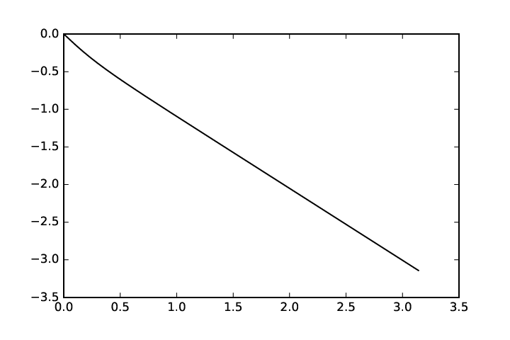
In Fig. 5, the graph of

is plotted for $r=4/5$ and $u$ varying from $-r$ to $-1$ (this parametrises the lower side of the cut counter-clockwise provided it is considered as a part of $\partial A_{r}$; see Fig. 2). According to (38), this gives the right-hand side of $\Gamma$ shown in Fig. 3. Since (41) is a monotonic function, there is no violation of the boundary correspondence on the right-hand side of $\Gamma$.

Finally, the graph of the first function (34) is plotted in Fig. 6 for $r=4/5$ and $t$ varying from $0$ to $\pi$ (this parametrises the upper half of the exterior circumference of $\partial A_{r}$ counter-clockwise; see Fig. 2). According to the first equation (34), this parametrises the left-hand part of the upper side of $\Gamma$ shown in Fig. 3. Since (34) is a monotonic function, there is no violation of the boundary correspondence on this part of $\Gamma$.

It remains to check that $\Omega$ is a one-wave domain for some Stokes wave; that is, there exists a stream function $\psi$ defined on $\overline{\Omega}$ so that it satisfies conditions (11)–(13) with some constant serving as the right-hand side term in (11), whereas $\mu$ stands in (13). For this purpose we map $\Omega$ conformally on an auxiliary rectangle

so that the images of $z_{s}$ and $z_{b}$ are the top and bottom parts of $\partial R^{*}$ respectively, whereas the value $\psi_{0}>0$ will be be chosen later. Thus, there are harmonic functions $\varphi^{*}$ and $\psi^{*}$ defined on $\Omega$, and for every $\psi_{0}$ the image of $R^{*}$ under the mapping $\textrm{e}^{-\kern 0.40974pt\mathrm{i}\kern 0.40974pt(\varphi^{*}+\kern 0.40974pt\mathrm{i}\kern 0.40974pt\psi^{*})}$ is the annular domain $A_{\rho}$ with some $\rho$. It is clear that the value of $\rho$ decreases from unity to zero as $\psi_{0}$ characterising $R^{*}$ increases from zero to infinity. Requiring $\rho$ to be equal to $r$, we fix the value of $\psi_{0}$, thus determining $\psi^{*}$ which, in its turn, gives the constant value $-Q_{*}$ that stands on the right-hand side of condition (11); here the sign is chosen so that $Q_{*}$ is positive. It should be noted that this procedure guarantees that condition (12) is also fulfilled. It remains to use $\varphi^{*}$ and $\psi^{*}$ for determining $\psi$ so that it satisfies condition (13) along with (11) and (12).

Using the Fourier coefficients $b_{1},b_{2},\dots$ of $v$ in formula (25), we obtain the function $z_{\varphi^{*}}$ holomorphic in $A_{r}$ and non-vanishing there. According to equation (28), we have that

is the limit as $|u|\to 1$ of some holomorphic function given in $A_{r}$ and having its imaginary part equal to zero on $\partial A_{r}\cap\{|u|=r\}$. Besides, the same property holds for $z_{\varphi^{*}}$, and so it is also true for the function whose limit as $|u|\to 1$ is equal to

Therefore, we have that

with some $q>0$ and $\eta$ defined above. For $\psi=q\sqrt{\mu}\,\psi^{*}$ the last relation coincides with (13).

Thus, the triple $(\mu,\eta,\psi)$ satisfies problem P$(Q_{0},h)$ with $h$ defined by (36), whereas $Q_{0}=q\sqrt{\mu}\,Q_{*}$ and $Q_{*}$ depends on $r$ implicitly as described above. This completes the description of a procedure how to obtain a solution of problem (10)–(13) from the given solution of Babenko’s equation.

Let $r\in[0,1)$ be fixed, then $J_{r}=\mathcal{B}_{r}\mathrm{d}\kern 0.2pt/\mathrm{d}\kern 0.2ptt$ is a self-adjoint operator on $L^{2}_{per}(-\pi,\pi)$ of $2\pi$-periodic square integrable functions. Its domain is $H_{0}$ (see Section 3.2 for the definition), and it can also be defined by linearity from $J_{r}\cos nt=\lambda_{n}\cos nt$ for $n=0,1,\dots$ and $J_{r}\sin nt=\lambda_{n}\sin nt$ for $n=1,2,\dots$; here the eigenvalues are $\lambda_{n}=\mu_{n}^{-1}$ for $n\geqslant 1$ and $\lambda_{0}=0$; cf. (31). Since the corresponding eigenfunctions form a basis in $L^{2}(-\pi,\pi)$, the following spectral decomposition holds:

Here $\hat{P}_{n}$ $(\tilde{P}_{n})$ is the projector onto the subspace spanned by $\cos nt$ ($\sin nt$, respectively).

Seeking solutions of (28) in $\hat{H}_{0}$, it is convenient to write the equation in an equivalent form to accelerate numerical calculations. This form arises after replacing $J_{r}$ in (28) by the right-hand side of (42) with omitted $\tilde{P}_{n}$, which is possible in view of the bijection between $\hat{H}_{0}$ and the Sobolev space $W^{1,2}(0,\pi)$; indeed, for every $w\in W^{1,2}(0,\pi)$ its even extension $v$ belongs to $\hat{H}_{0}$ and vice versa. Therefore, it is convenient to put $\mathcal{J}_{r}=\sum_{n=1}^{\infty}\lambda_{n}P_{n}$, where $P_{n}$ is the projector onto the subspace of $L^{2}(0,\pi)$ spanned by $\cos nt$. Then $\mathcal{J}_{r}$ is defined on $W^{1,2}(0,\pi)$ and $\mathcal{J}_{r}w=J_{r}v(=\mathcal{B}_{r}v^{\prime})$ almost everywhere on $(0,\pi)$, and so (28) takes the following equivalent form

References

- [1] A. L. Afendikov, L. R. Volevich, G. P. Voskresenskii, I. M. Gelfand, A. V. Zabrodin, O. V. Lokutsievskii, O. A. Oleinik, V. M. Tikhomirov, N. N. Chentsov, Konstantin Ivanovich Babenko (obituary). Russian Math. Surveys 43 (1988), 139–151.
- [2] K. I. Babenko, Some remarks on the theory of surface waves of finite amplitude. Soviet Math. Doklady 35 (1987), 599–603.
- [3] K. I. Babenko, A local existence theorem in the theory of surface waves of finite amplitude. Soviet Math. Doklady 35 (1987), 647–650.
- [4] K. I. Babenko, V. Yu. Petrovich, A. I. Rakhmanov, A computational experiment in the theory of surface waves of finite amplitude. Soviet Math. Doklady 38 (1989), 327–331.
- [5] K. I. Babenko, V. Yu. Petrovich, A. I. Rakhmanov, On a demonstrative experiment in the theory of surface waves of finite amplitude. Soviet Math. Doklady 38 (1989), 626–630.
- [6] G. G. Stokes, On the theory of oscillatory waves. Camb. Phil. Soc. Trans. 8 (1847), 441–455.
- [7] P. I. Plotnikov, J. F. Toland, Convexity of Stokes waves of extreme form. Arch. Ration. Mech. Anal. 171 (2004), 349–416.
- [8] A. I. Nekrasov, On steady waves. Izvestia Ivanovo-Voznesensk. Politekhn. Inst. 3 (1921), 52–65; also Collected Papers, I. Izdat. Akad. Nauk SSSR, 1961, pp. 35–51 (both in Russian).
- [9] A. I. Nekrasov, The Exact Theory of Steady Waves on the Surface of a Heavy Fluid. Izdat. Akad. Nauk SSSR, 1951; also Collected Papers, I. Izdat. Akad. Nauk SSSR, 1961, pp. 358–439 (both in Russian); translated as University of Wisconsin MRC Report no. 813, 1967.
- [10] A. I. Nekrasov, On steady waves on the surface of a heavy fluid. Proc. All-Russian Congr. of Matematicians, Moscow, (1928), 258–262 (in Russian).
- [11] C. J. Amick, J. F. Toland, On periodic water-waves and their convergence to solitary waves in the long-wave limit. Phil. Trans. Roy. Soc. Lond. A 303 (1981), 633–669.
- [12] T. Levi-Civita, Détermination rigoureuse des ondes permanentes d’amplieur finie. Math. Ann. 93 (1925), 264–314.
- [13] D. J. Struik, Détermination rigoureuse des ondes périodiques dans un canal à profondeur finie. Math. Ann. 95 (1926), 595–634.
- [14] E. Zeidler, Nonlinear Functional Analysis and its Applications, IV. Springer-Verlag 1987.
- [15] E. Zeidler, Nonlinear Functional Analysis and its Applications, I. Springer-Verlag, 1985.
- [16] B. Buffoni, J. F. Toland, Analytic Theory of Global Bifurcation: an Introduction. Princeton University Press, Princeton 2003.
- [17] J. F. Toland, Stokes waves. Topol. Methods Nonlinear Anal. 7 (1996), 1–48. Errata. Ibid 8 (1997), 412–413.
- [18] Yu. P. Krasovskii, On the theory of steady waves of finite amplitude. USSR Comput. Math. Math. Phys. 1 (1961), 996–1018.
- [19] B. Buffoni, E. N. Dancer, J. F. Toland, The regularity and local bifurcation of steady periodic waves. Arch. Ration. Mech. Anal. 152 (2000), 207–240.
- [20] B. Buffoni, E. N. Dancer, J. F. Toland, The sub-harmonic bifurcation of Stokes waves. Arch. Ration. Mech. Anal. 152 (2000), 241–271.
- [21] H. Okamoto, M. Shōji, The Mathematical Theory of Permanent Progressive Water-Waves. World Scientific, Singapore 2001.
- [22] A Zygmund, Trigonometric Series, I & II. Cambridge University Press, Cambridge 1959.
- [23] E. Shargorodsky, J. F. Toland, Bernoulli free-boundary problems. Memoirs AMS 96 (2008), no. 914.
- [24] M. S. Longuet-Higgins, Some new relations between Stokes’s coefficients in the theory of gravity waves. J. Inst. Maths. Applics. 22 (1978), 261–273.
- [25] J. G. B. Byatt-Smith, The equivalence of Bernoulli’s equation and a set of integral relations for periodic waves. IMA J. Appl. Math. 23 (1979), 121–130.
- [26] M. S. Longuet-Higgins, Bifurcation in gravity waves. J. Fluid Mech. 151 (1985), 457–475.
- [27] A. M. Balk, A Lagrangian for water waves. Phys. Fluids 8 (1996), 416–420.
- [28] M. S. Longuet-Higgins, Lagrangian moments and mass transport in Stokes waves. Part 2. Water of finite depth. J. Fluid. Mech. 186 (1988), 321–336.
- [29] B. Chen, P. G. Saffman, Numerical evidence for the existence of new types of gravity waves of permanent form on deep water. Stud. Appl. Math. 62 (1980), 1–21.
- [30] J.-M. Vanden-Broeck, Some new gravity waves in water of finite depth. Phys. Fluids 26 (1983), 2385–2387.
- [31] J.-M. Vanden-Broeck, L. W. Schwartz, Numerical computation of steep gravity waves in shallow water. Phys. Fluids 22 (1979), 1868–1873.
- [32] W. Craig, D. P. Nicholls, Travelling gravity water waves in two and three dimensions. European J. Mech. B/Fluids 21 (2002), 615–641.
- [33] J. A. Zufiria, Weakly nonlinear non-symmetric gravity waves on water of finite depth. J. Fluid Mech. 180 (1987), 371–385.
- [34] C. Baesens, R. S. MacKay, Uniformly travelling water waves from a dynamical systems viewpoint: some insights into bifurcations from Stokes’ family. J. Fluid Mech. 241 (1992), 333–347.
- [35] A. Constantin, W. Strauss, E. Vărvărucă, Global bifurcation of steady gravity water waves with critical layers. Acta Math. 217 (2016), 195–262.
- [36] T. B. Benjamin, Verification of the Benjamin–Lighthill conjecture about steady water waves. J. Fluid Mech. 295 (1995), 337–356.
- [37] V. Kozlov, N. Kuznetsov, The Benjamin–Lighthill conjecture for steady water waves (revisited). Arch. Ration. Mech. Anal. 201 (2011), 631–645.
- [38] V. Kozlov, N. Kuznetsov, Bounds for arbitrary steady gravity waves on water of finite depth. J. Math. Fluid Mech. 11 (2009), 325–347.
- [39] V. Kozlov, N. Kuznetsov, Fundamental bounds for steady water waves. Math. Ann. 345 (2009), 643–655.
- [40] T. B. Bodnar’, On steady periodic waves on the surface of a fluid of finite depth. J. Appl. Mech. Tech. Phys. 52 (2011), 378–384.
- [41] M. G. Crandall, P. H. Rabinowitz, Bifurcation from simple eigenvalues. J. Func. Anal. 8 (1971), 321–340.
- [42] M. Tanaka, The stability of steep gravity waves. J. Phys. Soc. Japan 52 (1983), 3047–3055.
- [43] P. G. Saffman, The superharmonic instability of finite amplitude water waves. J. Fluid Mech. 159 (1985), 169–174.
- [44] M. A. Evgrafov, Analytic functions. Dover, New York 1978.
- [45] D. Moldabayev, O. Verdier, H. Kalisch, SpecTraVVave 2018. Free software available at https://github.com/olivierverdier/SpecTraVVave
- [46] H. Kalisch, D. Moldabayev, O. Verdier, A numerical study of nonlinear dispersive wave models with SpecTraVVave. Electronic J. Diff. Equations 2017 (2017), 1–23.
- [47] P. J. Aston, Analysis and computation of symmetry-breaking bifurcation and scaling laws using group theoretic methods. SIAM J. Math. Anal. 22 (1991), 181–212.
- [48] J. A. Zufiria, Non-symmetric gravity waves on water of infinite depth. J. Fluid Mech. 181 (1987), 17–39.
- [49] A. Constantin, E. Vărvărucă, Steady periodic water waves with constant vorticity: regularity and local bifurcation. Arch. Ration. Mech. Anal. 199 (2011), 33–67.