Fractal Dimension of the Kronecker Product Based Fractals

The Kronecker product [1] generates fractals if it applies to the same matrix [1-3], i.e., it is the self Kronecker product.

The origin, nature and generating technique related to the Kronecker product based (KPB) fractals are explained in more details in [2,3]. A lot of well-known and new fractal samples are shown and KPB fractals generators are offered both in JavaScript and in R [2,3].

A simple method of calculating the Hausdorff-Besicovitch dimension (HBD) of the Kronecker Product based fractals was discovered and is presented together with a compact R script realizing it. The proposed new formula is based on traditionally used values of the number of self-similar objects and the scale factor that are now calculated using appropriate values of both the initial fractal matrix and the second order resultant matrix. This method is reliable and producing dimensions equal to many already determined values of well-known canonical fractals.

It should be stressed in the beginning that this method only works and could be applied to any fractal matrix (defined below) to determine KPB fractal dimension.

Let’s start with a few definitions that are related and applied only to matrices used for fractal images generation using a self Kronecker product (a.k.a. the Kronecker power).

Note: a matrix declared an “initial” has the order 1, even if it is, in fact, a resultant order $N$ matrix generated previously.

For clarity, a simple notation is used to stress the name of the fractal (using abbreviation) and its order (in the form ‘oN’). E.g., for the Sierpinski triangle fractal (STF) order 7 – both generated matrix and plotted picture would be denoted as STFo7.

Here is another important definition:

Some initial matrices (even fractal ones) can’t, produce fractals. So, here is a definition for them:

To generate and plot KPB fractals R helper functions from [3] will be use. It should be explained that R helper functions just simplifying and standardizing generating and plotting for fractal matrices. But, in fact, R language has a built-in operator $\%x\%$ for the Kronecker product, i.e., for any matrix $M$ it could be used as $M\%x\%M$.

To start, two Sierpinski canonical fractals – triangle and carpet – are shown in the figures below.

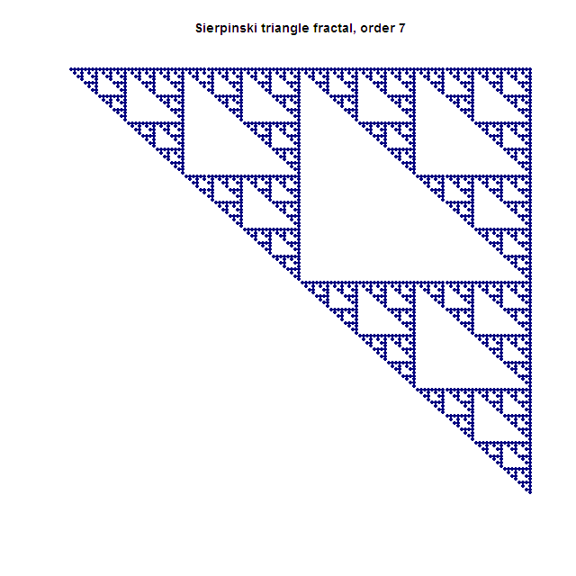
The initial fractal matrices for these two fractals and how to generate and plot them using helper functions from [3] is shown in the R script #1 below.

Now, only matrices of the second order will be built (without plotting) in R.

Although R script output is very clear, in the Fig. 3, 4 below find the initial, second and third order matrices plotted using big square “dots”. This makes it even easier to determine the basic figure, counting and scaling.

A very simple formula to calculate Hausdorff-Besicovitch dimension of the fractal $F$ was introduced in [5] and further explain in [6,7] and it fits our goal:

Let’s apply the above formula to the Sierpinski triangle fractal. Looking at Fig. 3 we can find that in the order 2 matrix the number of self-similar objects (i.e., objects equal to the basic one in the initial matrix) $N=3$, and the scale factor $S=2$. So, $\dim_{\mathrm{HB}}STF=log3/log2=1.584963$.

Applying the same formula to the Sierpinski carpet fractal (see Fig. 4) we have: the number of self-similar objects $N=8$, the scale factor $S=3$ and
$\dim_{\mathrm{HB}}SCF=log8/log3=1.892789$.

As result of intensive testing, it was discovered that in case of KPB fractals:

• •

  $N$ is the ratio $d2/d1$, where $d2$ is a number of dots in the resultant matrix of the second order and $d1$ is a number of dots in the initial matrix.

• •

  $S$ is the ratio $m2/m1$, where $m2$ is a number of rows in the resultant matrix of the second order and $m1$ is a number of rows in the initial matrix.

The new simple formula to calculate Hausdorff-Besicovitch dimension of the fractal $F$ is the following:

Such amazing simplicity could be explained by the fact that the Kronecker product is building resultant block-matrix in a uniform manner, so, these two ratios are always describing correctly both the number of self-similar objects and the scale factor. Moreover, these ratios are the same between other orders, e.g., between the second and third orders, etc.

Based on this discovered formula, – a very simple R script was created. Just 7 lines of R code:

R script dimHB4kpf.R

    ## dimHB4kpf.R.txt 3/11/17 aev
    ## Hausdorff-Besicovitch dimension for Kronecker product based
    ## fractals
    ## Note: only for Kronecker product based fractals created from
    ## the fractal matrix!
    ## dimHB4kpf(mat, ttl) -
    ## where: mat - initial matrix (filled with 0/1); ttl - title.
    dimHB4kpf <- function(mat, ttl="") {
      m1 = nrow(mat); dn1 = sum(mat!=0);
      matr = mat%x%mat; ##self Kronecker product
      m2 = nrow(matr); dn2 = sum(matr!=0);
      dimHB = log(dn2/dn1, m2/m1);
      cat(" *** dimHB:", dimHB, ttl, "\n");
    }

Presented below testing R script #3 is pretty simple. It includes two lines of code for each of 7 selected well-known fractals.

Note: last 5 fractals are shown in the Fig. 5-9 below.

Results of the testing script are presented below, and they are equal to results shown in [8] for the same fractals.

The discovered new simple formula to calculate the Hausdorff-Besicovitch dimension together with offered compact R script (dimHB4kpf.R) can help studies related to KPB fractals and even to any fractals in general.

For example, if any fractal can be simulated using matrix presentation and the Kronecker power, then its Hausdorff-Besicovitch dimension can be calculated instantly, - helping understand many peculiarities of this fractal.

Actually, it was done already here for Hexagon fractal (see Fig. 8). Our plotted Hexagon fractal is very similar to the Hexaflake in [8], but it looks rather as a distorted Hexaflake. Anyway, they both have the equal dimension.

Here is another appropriate and interesting example related to the Rauzy gasket (RG) described in [9]. The authors of [9] proved “that the Rauzy gasket is homeomorphic to the usual Sierpinski gasket”. If compare the Fig. 1 in the mentioned article (which is presented the Rauzy gasket) and the Fig. 1 above (presented Sierpinski triangle fractal, aka Sierpinski gasket), - it is very clear that the RG is looking like a distorted version of STF, and it is actually copying the structure of STF.

It was already calculated that $\dim_{\mathrm{HB}}STF=1.584963$, so $\dim_{\mathrm{HB}}RG$ is the same (at least, expected to be almost the same). This value is in accordance with the fact proved in [10]: “the Hausdorff dimension of the Rauzy gasket is less than 2”. One can look at this value as a reasonable approximation, until the precise value would be found, or it would be proved that dimensions of both gaskets are equal.

References

- [1] Steeb, W.-H. (2006), Problems and Solutions in Introductory and Advanced Matrix Calculus, World Scientific Publishing. pp. 152–173. ISBN 981-256-916-2.
- [2] Voevudko, A.E. (2017), Generating Kronecker Product Based Fractals, Code Project, URL: https://www.codeproject.com/Articles/1189288/ Generating-Kronecker-Product-Based-Fractals.
- [3] Voevudko, A.E. (2017), A Few Approaches to Generating Fractal Images in R, Code Project, URL: https: //www.codeproject.com/Articles/ 1195034/A-Few-Approaches-to-Generating-Fractal-Images-in-R.
- [4] Kronecker product based fractals, Rosetta Code Wiki, URL: http://rosettacode.org/ wiki/Kronecker_product_ based_fractals.
- [5] Falconer, K.J. (1990), Fractal geometry: mathematical foundations and applications. John Wiley and Sons, New York, doi:10.2307/2532125.
- [6] Fractal dimension, Wikipedia, the free encyclopedia, URL: https:// en.wikipedia.org/wiki/Fractal_dimension.
- [7] Hausdorff dimension, Wikipedia, the free encyclopedia, URL: https:// en.wikipedia.org/wiki/Hausdorff_dimension.
- [8] List of fractals by Hausdorff dimension, Wikipedia, the free encyclopedia, URL: https://en.wikipedia.org/wiki/List_of_fractals_by_Hausdorff_dimension.
- [9] P. Arnoux, S. Starosta (2013), The Rauzy Gasket. In: Barral J., Seuret S. (eds) Further Developments in Fractals and Related Fields. Trends in Mathematics, Springer, New York, doi:10.1007/978-0-8176-8400-6_1.
- [10] A. Avila, P. Hubert, A. Skripchenko (2015), On the Hausdorff dimension of the Rauzy gasket. arXiv:1311.5361v3 [math.DS].