Spheroidal and conical shapes of ferrofluid-filled capsules in magnetic fields
Abstract
We investigate the deformation of soft spherical elastic capsules filled with a ferrofluid in external uniform magnetic fields at fixed volume by a combination of numerical and analytical approaches. We develop a numerical iterative solution strategy based on nonlinear elastic shape equations to calculate the stretched capsule shape numerically and a coupled finite element and boundary element method to solve the corresponding magnetostatic problem, and employ analytical linear response theory, approximative energy minimization, and slender-body theory. The observed deformation behavior is qualitatively similar to the deformation of ferrofluid droplets in uniform magnetic fields. Homogeneous magnetic fields elongate the capsule, and a discontinuous shape transition from a spheroidal shape to a conical shape takes place at a critical field strength. We investigate how capsule elasticity modifies this hysteretic shape transition. We show that conical capsule shapes are possible but involve diverging stretch factors at the tips, which gives rise to rupture for real capsule materials. In a slender-body approximation we find that the critical susceptibility above which conical shapes occur for ferrofluid capsules is the same as for droplets. At small fields capsules remain spheroidal, and we characterize the deformation of spheroidal capsules both analytically and numerically. Finally, we determine whether wrinkling of a spheroidal capsule occurs during elongation in a magnetic field and how it modifies the stretching behavior. We find the nontrivial dependence between the extent of the wrinkled region and capsule elongation. Our results can be helpful in quantitatively determining capsule or ferrofluid material properties from magnetic deformation experiments. All results also apply to elastic capsules filled with a dielectric liquid in an external uniform electric field.
I Introduction
Elastic capsules consist of a thin elastic shell enclosing a fluid inside. Elastic microcapsules are found in nature, for example, as red blood cells or virus capsids. They can also be produced artificially by various methods, for example, interfacial polymerization at liquid-liquid interfaces or multilayer polyelectrolyte deposition [1]. Artificially produced microcapsules are attractive systems for encapsulation and transport, for example, in delivery and release systems. Their overall shape is often nearly spherical, and the shell can be treated as a two-dimensional elastic solid with a curved equilibrium shape. In experiments and for applications, elastic properties of capsules can be tuned by varying size, thickness, and shell materials. For applications involving delivery by rupture of capsules it is necessary to understand and characterize the mechanical properties and elastic instabilities of capsules.
The mechanical properties of elastic capsules are governed by the elastic shell, which is curved (typically spherical) in its equilibrium shape. This gives rise to different characteristic instabilities in response to external forces [2, 3, 1]. Thin elastic membranes bend much more easily than stretch. This protects a curved equilibrium shape against deformations changing its Gaussian curvature and that is the reason for the stability of capsules under uniform compression. In contrast to fluid drops, elastic capsules under uniform compression fail in a buckling instability below a critical volume or critical internal pressure [4, 5, 6, 7, 8, 9]. Buckling-type instabilities can also be triggered by external forces, for example, in electrostatically driven buckling transitions of charged shells [10] or in hydrodynamic flows [11]. Under point force loads, for example, exerted by atomic force microscopy tips, elastic capsules indent linearly at small forces and assume buckled shapes in the nonlinear regime at higher forces [2, 12, 13]. As opposed to fluid droplets, elastic capsules can also develop wrinkles upon deformation [14, 15, 16, 17] if compressive hoop stresses arise.
Microcapsules can be manipulated and deformed in hydrodynamic flow [18, 14, 19], by micromanipulation using an atomic force microscope [2, 3] or micropipettes or capillaries [16, 17]. Another promising route to exert mechanical forces and to actuate elastic capsules in a noninvasive manner is via magnetic or electric fields [20, 21]. For magnetic fields this requires the presence of magnetizable material either in the shell or in the capsule interior. The whole capsule then acquires a magnetic dipole moment, which can be manipulated in external magnetic fields. For actuation by electric fields the capsule has to contain polarizable dielectric material such that the capsule acquires an electrostatic dipole moment, which can be manipulated by an electric field. Homogeneous fields orient dipole moments but also induce capsule deformations, which increase the size of the dipole moment after orientation. Therefore, homogeneous fields always lead to stretching and elongation of the capsule. Inhomogeneous fields can also exert a net force on the capsule and induce directed motion at fixed magnetic dipole moment along the field gradient.
In the following we focus on spherical elastic capsules that are filled with a (quiescent) magnetic fluid and deformed in homogeneous external magnetic fields. As magnetic fluid we consider a ferrofluid, which is a liquid that is magnetizable by external magnetic fields because it consist of ferromagentic or ferrimagnetic nanoparticles suspended in a carrier fluid. Because of the small particle size, ferrofluids are stable against phase separation and show superparamagnetic behavior [22]. Ferrofluids are used in technical and medical applications [23, 24, 25]. All our results also apply to elastic capsules filled with a (quiescent) dielectric fluid which are placed in a homogeneous external electric field.
The problem of ferrofluid droplets in uniform external magnetic fields has already been theoretically studied in the literature. Also, a spherical ferrofluid droplet is elongated in the direction of the magnetic field for increasing field strength; the resulting elongated shape was observed to be nearly spheroidal [26]. Bacri and Salin [27] used the assumption of a spheroidal shape for a quite precise approximation of the elongation by minimizing the total energy. Although the droplet is only elongated by the field, an abrupt shape transition is possible [27]: Beyond a threshold magnetic field strength the spheroidal droplet becomes unstable and elongates discontinuously into a shape with conical tips. The conical shape is stabilized by a positive feedback between shape and magnetic field distribution: A sharp tip gives rise to a diverging field strength at the tip, which in turn generates strong stretching forces stabilizing the sharp tip. The mechanism of forming sharp tips is reminiscent of the normal field instabilities (Rosensweig instabilities) of free planar ferrofluid surfaces in a perpendicular homogeneous magnetic field, which were first described by Cowley and Rosensweig [28] and later extended by a nonlinear stability analysis to study subsequent pattern formation [29].
The discontinuous shape transition to a conical shape exhibits hysteresis and only occurs above a critical susceptibility of the ferrofluid. In Refs. [30, 31] a value was found below which no conical shape can exist; a slender-body approximation in Ref. [32] gives . Using the approximative energy minimization for spheroidal shapes of Bacri and Salin [27] gives . The jump in droplet elongation at the transition to a conical shape depends on the magnetic susceptibility: Large elongation jumps are possible for high susceptibilities. This behavior was investigated in more detail in several numerical studies [33, 34, 35]. Apart from free ferrofluid droplets, the deformation behavior of sessile droplets on a plate [36] or sedimenting ferrofluid drops in external fields [37] have also been investigated for homogeneous external magnetic fields.
Dielectric droplets in a homogeneous external electric field exhibit the same shape transition from a spheroidal to a conical shape. For the electric field, however, free charges exist, and conducting droplets are easily realized experimentally. In fact, the first experimental observations of conical droplet shapes were made for water droplets [38] and soap bubbles [39]. In Ref. [31] it was shown that also a conducting liquid droplet surrounded by an outer conducting liquid in a homogeneous electric field exhibits conical shapes above a corresponding critical conductivity ratio . In the limit of an ideally conducting droplet with infinite susceptibility or infinite conductivity (both resulting in zero electric field inside the droplet), the conical solutions in Refs. [30, 31, 32] approach Taylor’s cone solution with a half opening angle [40]. Both for liquid metal (i.e., ideally conducting) and dielectric droplets, the conic cusp formation has been studied dynamically and dynamic self-similar solutions have been obtained [41, 42]. Fluid droplets, which are neither perfect conductors nor perfect insulators, disintegrate at higher external electric fields by emitting jets of fluid at the tip, from which small droplets pinch off. Also for this process, scaling laws for droplet sizes could be theoretically obtained [43, 44].
In a ferrofluid-filled elastic capsule the ferrofluid drop is enclosed by a thin elastic membrane, which will modify the transition from a spheroidal to a conical shape observed for droplets. Such ferrofluid-filled capsules have already been realized experimentally. Neveu-Prin et al. [45] encapsulated ferrofluids by polymerization and analyzed the magnetization behavior of the magnetic capsules. Degen et al. [20] investigated experimentally elastic capsules filled with a magnetic liquid in an external magnetic field. They used a magnetic liquid consisting of micrometer-sized magnetic particles that do not show the special properties of ferrofluids but form long chains in the presence of external magnetic fields. These magnetite-filled elastic capsules could be actuated to deform in a magnetic field. A quantitative theoretical description of their deformation is still missing. In Ref. [21], capsules filled with a dielectric liquid in an external electric field were investigated experimentally and theoretically with a focus on small deformations.
We will describe the elastic shell by a nonlinear elastic model based on a Hookean elastic energy density for thin shells, assume axisymmetric capsules, and calculate the shape at force equilibrium by solving shape equations as they have been derived in Refs. [7, 17]. As stated above, homogeneous magnetic fields acting on ferrofluid-filled capsules give rise to stretching and elongation of the capsule in order to increase the total dipole moment. Therefore, stretching tensions are dominant in the elastic shell. This is why we will consider the limiting case of vanishing bending modulus and bending moments for most of the present work, which is commonly called the elastic membrane limit (as opposed to the elastic shell case).
In our numerical approach, the magnetic field inside the capsule is calculated using a coupled finite element and boundary element method. The capsule shape provides the geometric boundary for the field calculation. Vice versa, the magnetic field distribution couples to the shape equations via the magnetic surface stresses. We solve the full coupled problem numerically by an iterative method.
We combine this numerical approach with several analytical approaches to investigate the capsule deformation in a homogeneous magnetic field as a function of the magnetic field strength and Young modulus of the capsule material. First we characterize the linear deformation regime of spheroidal capsules for small fields both numerically and analytically. Then we answer the question to what extent the elastic shell will suppress the discontinuous spheroidal to conical shape transition of a ferrofluid droplet and whether elastic properties such as the Young modulus of the shell material can be used to tune and control the instability. We show that conical shapes can also occur for capsules with nonlinear Hookean membranes but require diverging strains at the conical tips. As a real elastic material is not able to support arbitrarily high strains, we expect that diverging local stretch factors at the capsule poles indicate that real capsules tend to rupture close to the poles as soon as the conical shape is assumed. Then the existence of a sharp discontinuous shape transition into a conical shape provides an interesting route to trigger capsule rupture at the poles at rather well-defined magnetic (for ferrofluid-filled capsules) or electric (for dielectric-filled capsules) field values. The subsequent rupture process has some analogies to the onset of the disintegration of droplets in electric fields [43, 44], but our static approaches based on nonlinear Hookean material laws are not suited to model the rupture process itself.
We find that the discontinuous shape transition between spheroidal and conical shapes with hysteresis effects and shape bistability is also present for elastic ferrofluid-filled capsules. Numerically, we obtain a complete classification of the shape transition in the parameter plane of dimensionless magnetic field strengths (magnetic Bond number) and the dimensionless ratio of the Young modulus of the shell material and the surface tension of the ferrofluid. These findings are partly corroborated by an analytical approximative energy minimization extending the spheroidal shape approximation of Bacri and Salin [27] to ferrofluid-filled capsules. For conical shapes we generalize the slender-body approximations of Stone et al. [32], which allows us to quantify the divergence of local stretch factors at the capsule poles and to show that the same analytic formula as for ferrofluid droplets governs the dependence of the cone angle on the magnetic susceptibility (or the dielectric susceptibility for a dielectric droplet with dielectric constant in a surrounding liquid with ). In particular, we predict the critical susceptibility , above which the hysteretic shape transition between spheroidal and conical capsule shapes can be observed, to be identical to the critical value for ferrofluid or dielectric droplets. We also find that, for elastic capsules, magnetic stretching can give rise to wrinkling along the capsule equator region. We predict the parameter range for the appearance of wrinkles and the extent of the wrinkled region on a spheroidal capsule depending on its elastic properties and its elongation.
II Theoretical model and numerical methods
We start with a ferrofluid drop suspended in an external nonmagnetic liquid of the same density as the ferrofluid, which eliminates gravitational forces. Thus the drop is force-free except for the surface tension , which forces the drop to be spherical and is balanced by internal pressure. If the drop is enclosed by an elastic shell, for example, after a polymerization reaction at the liquid-liquid interface, we have a spherical elastic capsule. We assume that the relaxed rest shape of this capsule is spherical with a rest radius , which is given by the fixed volume of the droplet or capsule.
After applying a uniform magnetic field in the direction, the resulting shape of the capsule becomes stretched in the direction, but the capsule shape and magnetic field distribution remain axisymmetric around the axis. A uniform external magnetic field causes mirror-symmetric forces on the capsule, resulting in a shape with reflection symmetry with respect to the plane (see Fig. 1).
II.1 Geometry
We describe the axisymmetric shell using cylindrical coordinates , , and . The capsule’s shell is thin compared to its diameter, so we consider the shell to be a two-dimensional elastic surface. Because of the axial symmetry, we only need the contour line to describe the whole capsule shape.
For our calculations, we parametrize the surface by the arc length of the undeformed spherical contour with , starting at the lower apex and ending at the upper apex. Using the reflection symmetry, we only need half of that interval, , to describe the capsule’s shape completely. In addition to the coordinates and , we define a slope angle by the unit vector following the contour line via .

II.2 Magnetostatics
II.2.1 Forces by the ferrofluid
In order to calculate the shape of the capsule in an external magnetic field, we have to take the magnetic forces that are caused by the ferrofluid on the capsule surface into account. Because we are interested in a static solution, we can assume that the fluid is at rest. Then the fluid can only exert hydrostatic forces normal to the surface, while tangential components are zero. In order to calculate the normal magnetic force density on the surface, we use the magnetic stress tensor by Rosensweig, [22]
| (1) |
Here is the absolute value of the magnetization and its normal component ( is the outward unit normal to the capsule surface). Magnetization and magnetic field are taken on the inside of the capsule surface.
We assume a linear magnetization law
| (2) |
with a susceptibility for the ferrofluid ( in terms of its magnetic permeability ), which is justified for small fields , where is the saturation magnetization of the ferrofluid. References [46, 47] studied the behavior of drops with a nonlinear Langevin magnetization (polarization) law. The saturation of the magnetization or polarization forbids sharp tips and leads to more rounded drops. It was shown, on the other hand, that the linear law is a very good approximation for small and even medium fields. This typically requires the maximum magnetic flux density to be in a range of , depending on the specific fluid [48, 36]. For a linear magnetization we can rewrite Eq. (1) as
| (3) |
(assuming for the external non-magnetic liquid or using in terms of the magnetic permeabilities of the ferrofluid and the of the external liquid), where and is the normal component of the magnetic field. We will use this position-dependent normal magnetic force density to modify the pressure in our elastic equations in Sec. II.3.1.
II.2.2 Calculation of the magnetic field
To calculate the total magnetic field, i.e., the superposition of the external uniform field and the field from the ferrofluid magnetization, we use the fact that ferrofluids are generally non-conducting [22]. Then Maxwell’s equations give , which allows us to introduce a scalar magnetic potential with . From Maxwell’s equation we get Poisson’s equation in magnetostatics
| (4) |
For the linear magnetization law (2), Poisson’s equation simplifies to the Laplace equation .
For the numerical solution of this partial differential equation we use a coupled axisymmetric finite element – boundary element method [49, 50, 51, 52] with a cubic spline interpolation for the boundary [53]. This combination of methods was also used by Lavrova et al. for free ferrofluid drops [34, 54, 55] and earlier for electric drops, e.g., by Harris and Basaran [56]. The finite element method (FEM) is used to solve Eq. (4) in the magnetized domain inside the capsule and the boundary element method (BEM) for the nonmagnetic domain outside. Both domains are coupled by the continuity conditions of magnetostatics for and its normal derivative on the boundary of the capsule,
| (5) |
with for the external nonmagnetic liquid. Both the FEM and BEM exploit axial symmetry and effectively operate in the two-dimensional plane, where the axisymmetric capsule shape is described by a contour line . For the FEM we use a standard Galerkin method with linear elements on a triangular two-dimensional grid in the plane that is created with a Delauney triangulation using the Fade2D software package [57], where we set a fixed number of grid points on the capsule’s boundary.
In the BEM we express solutions of the Laplace equation for on the outside or the boundary of the capsule in terms of integrals over the boundary of the capsule. Using fundamental solutions with rotational symmetry [58], we have to solve a set of one-dimensional integrals over the whole boundary of the capsule
| (6) |
Here is the axially symmetric fundamental solution of Laplace’s equation, which is obtained from the fundamental solution of Laplace’s equation, . In the integral equation (6), and its normal derivative are evaluated on the outside of the capsule surface. The point is the point where is to be calculated, while the integrals are taken over points on the capsule contour. Both and lie in the same -plane. For the geometric factor , we have for points on the boundary and for points in the exterior domain. The vector denotes the outward unit normal vector and describes the -component of . On the right-hand side of (6), can be interpreted as the potential of the external electric field. For numerical evaluation, the integrals in Eq. (6) are discretized by a point collocation method and solved by applying Gaussian quadrature for nonsingular integrands and a midpoint rule for weakly singular integrands.
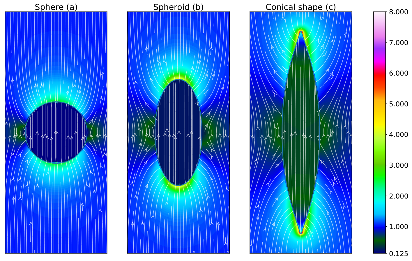
The FEM and BEM are coupled at the boundary by the continuity conditions (5). The FEM provides values for on every finite element grid point inside the capsule including values on the inner side of the boundary; in addition, the normal derivatives on the inside of the discretized capsule boundary are needed for the FEM but remain a priori unknown. Values for these normal derivatives on the boundary points of the FEM grid are obtained by the BEM method. Our BEM uses linear interpolation for between the discretized boundary points. We use the continuity conditions (5) to write the boundary integral equation (6) in terms of quantities on the inner capsule boundary. Using one BEM equation (6) for each boundary point (with ), we obtain a set of equations that allows us to calculate the unknown derivatives for given and to get a closed system of equations for everywhere inside the capsule. After solving the resulting system of FEM equations we know everywhere inside the capsule. For the calculation of inside the capsule and thus for the calculation of the magnetic force density acting on the capsule using (3), which is also calculated with the magnetic field on the inside, it is not necessary to calculate in the entire external domain explicitly. This is done implicitly by the BEM. If needed (for example, in order to calculate the field in the exterior regions in Fig. 2), can be calculated by solving (6) for points in the exterior with .
In a ferrofluid capsule or drop with sharp edges, very high field strengths can arise [see Fig. 2(c)]. Also field gradients can be large, which makes pointed shapes prone to discretization errors caused by the grid. This effect can be countered to some degree by placing more FEM grid points at the tip in order to improve the precision there, which is, however, limited by the BEM part of the solution scheme: The collocation points must not come too close to the symmetry axis because the weakly singular integrals become strongly singular on the axis [59]. This leads to massively increasing numerical errors near the axis and a decrease of the overall precision. Overall, our numerical scheme to calculate singular BEM integrals is not the most advanced as a trade-off for simplicity. There are more elaborated schemes for the integration of singular integrals as, for example, developed over many years by Gray et al. [60, 61], which could provide a more elegant way to deal with the problem. We use the following compromise for the discretization: We place elements on the boundary such that the length of the th boundary element (beginning at the equator) is given by
| (7) |
The constant is chosen in order to obtain the correct total arc length , which is given by the meridional stretch factors of the deformed capsule [see Eq. (11) below], . We choose ( gives a constant element length and leads to a higher element density at the capsule’s tip). Increasing beyond 250 does not improve the precision significantly. A higher density of points at the capsule’s tip (lower ) leads to stronger oscillations in the iterative solution scheme (see Sec. II.4 below).
II.2.3 Electric fields and dielectric liquid
Our approach to elastic capsules filled with a ferrofluid in a magnetic field also applies to capsules filled with a dielectric fluid in an electric field. The generic situation for a capsule filled with a fluid with dielectric constant is to be suspended in a dielectric liquid with a different , which does not equal unity . Then the dielectric force density in a linear medium is
| (8) |
which is completely analogous to (3) with playing the role of the susceptibility . For the general case, Poisson’s equation becomes
| (9) |
with the electric potential and the polarization . For a linear polarization law, it simplifies to the Laplace equation .
II.3 Equilibrium shape of the capsule
II.3.1 Elasticity and shape equations
The capsule is deformed by the normal magnetic stresses from the ferrofluid. We have to calculate the resulting deformed equilibrium shape, where all elastic stresses, surface tension and magnetic stress are balanced everywhere on the capsule. Every point of the reference shape is mapped onto a new point . The deformed shape is calculated by solving shape equations, which are derived from nonlinear theory of thin shells [62, 63, 7, 17]. We use a Hookean elastic energy density with a spherical rest shape. The Hookean elastic energy density (defined as energy per undeformed unit area) is given by
| (10) |
Here and are meridional and circumferential strains that contain the stretch factors and :
| (11) |
Here and in the following, quantities with subscript 0 refer to the undeformed spherical reference shape and quantities without 0 describe the deformed shape. Analogously, the bending strains and are generated by the curvatures and :
In the elastic energy (10), is the two-dimensional Young modulus governing stretching deformations, is the bending modulus, and is the two-dimensional Poisson ratio. Elastic properties are usually only weakly dependent; we use , which is the typical value for an incompressible polymeric material. The arc length of the deformed capsule’s contour is given by , while is the fixed arc length of the undeformed spherical capsule.
In experiments, the capsule’s shell is constructed by polymerization on the surface of a drop. Therefore, the undeformed reference shape, which is spherical in the absence of gravity, is also a solution of the Laplace-Young equation
| (12) |
where is the surface tension of the droplet. The solution of the Laplace-Young equation will be discussed in detail in Sec. II.3.4 below.
In the following, we will neglect the bending energy, which means we set . The characteristic length scale of the problem is the radius of the undeformed sphere, such that the neglect of the bending energy corresponds to the limit of large Föppl-von Kármán numbers . This is the limiting case of an elastic Hookean membrane and is a good approximation for two reasons. First, we will only consider capsules with thin shells as they were prepared in experiments [17, 20]. The shell thickness is very small compared to the capsule size, . With and it follows that and stretching energies are typically larger than bending energies. The second argument is that the homogeneous magnetic field acting on the ferrofluid-fluid capsule predominantly stretches and elongates the capsule in order to increase its total dipole moment. This increases stretching energies, whereas the capsules develop high curvatures only at the conical tips. However, we show below that stretch factors diverge at conical tips, so the stretching energy dominates over the bending energy associated with these high curvatures also in the tip regions.
Elastic tensions in the shell (defined as force per deformed unit length) derive from the surface elastic energy density by
| (13) | ||||
Although we use a Hookean elastic energy density, the constitutive relation (13) is nonlinear because of the additional factors, which arise for purely geometrical reasons: The Hookean elastic energy density is defined per undeformed unit area such that is the force per undeformed unit length, whereas the Cauchy stresses and are defined per deformed unit length.
In addition to the elastic tensions and , there is also a contribution from an isotropic effective surface tension between the outer liquid and the capsule. Such a contribution arises either as the sum of surface tensions of the liquid outside with the outer capsule surface and the liquid inside with the inner capsule surface or, if the capsule shell is porous such that there is still contact between the liquids outside and inside the capsule, with additional contributions from the surface tension between outside and inside liquids. In the absence of elastic tensions, the surface tension also gives rise to the spherical rest shape of the capsule. For macroscopic capsules the surface tensions should be negligible, but for microcapsules with weak walls they should not be neglected. We expect the effective surface tension to be somewhat smaller than typical liquid-liquid surface tensions, which are around ; we will use below.
The equilibrium of forces in the deformed elastic membrane is described by
| (14) | ||||
| (15) |
where Eq. (14) describes the normal force equilibrium and Eq. (15) tangential force equilibrium (in the direction, equilibrium in the direction is always fulfilled by axial symmetry). In the presence of magnetic forces, the pressure
| (16) |
is modified by the magnetic stress , which is a position-dependent normal stress pointing outwards and thus stretching the capsule and given by the magnetic field at the capsule surface [see Eq. (3)]. It is important to note that magnetic forces are always normal to the surface such that they do no enter the tangential force equilibrium (15). The (homogeneous) pressure is the Lagrange multiplier for the volume constraint .
The equations of force equilibrium and geometric relations can be used to derive a system of four first-order differential equations with the arc length of the undeformed spherical contour as an independent variable, which are called shape equations in the following:
| (17) | ||||
In these shape equations, the surface tension gives an isotropic and constant stress contribution, in addition to the elastic stresses and . This is because we assume that the undeformed rest state, where the elastic stresses and vanish, is identical to the shape of a ferrofluid droplet of surface tension . We neglect that could change during capsule preparation and during elastic deformation.
The system of shape equations is closed by the constitutive relation (13) for and the relations
where the first relation derives from the constitutive relation (13) for and the second relation is geometrical. For further details on the derivation of the shape equations, we refer the reader to Refs. [62, 17, 7].
II.3.2 Numerical solution of the shape equations
The system of shape equations (17) has to be solved numerically. The integration starts at the pole with and runs to the capsule’s equator at . To integrate the four first-order differential equations we have three boundary conditions at :
| (18) |
The condition for follows from the absence of holes in the capsule. We can choose arbitrarily because the external magnetic field does not depend on the coordinate. The boundary condition at the pole seems to exclude possible conical capsule shapes with . We discuss this issue below in Sec. III.3 and in Appendix C.3. There we derive the boundary condition for finite stretches and at the poles. The boundary condition also arises if the magnetic forces remain finite at the poles such that the normal force equilibrium requires finite curvatures at the poles. Conical shapes, however, have divergent stretches and and divergent magnetic normal forces at their conical tips. In the numerical calculation of capsule shape and magnetic field we have to discretize the capsule surface such that divergences are cut off (this numerical issue is discussed in more detail also in Appendix D) and the boundary condition for finite stretches and or finite magnetic force is appropriate. Then the right-hand side of the shape equation for in (17) vanishes, for [see also Eq. (71)], which can be used to start the integration at the pole. A priori, a fourth boundary condition for the tension at the pole is unknown. On the other hand, we have as a matching condition at to prevent kinks there. With the help of this matching condition, we can use a shooting method to determine . To increase numerical stability, we expand the shooting method to a multiple shooting method, where we use several integration intervals with several matching points.
To keep the volume of the capsule constant, we have to use the internal pressure as the Lagrange multiplier, which is adjusted during the calculation. In order to do so, becomes another shooting parameter with as the corresponding residual. In this work, we use a fourth order Runge-Kutta scheme with a step size of in the first integration interval starting at the apex and in all other intervals, while there is a total of 250 integration intervals.
II.3.3 Wrinkling
A ferrofluid-filled capsule is stretched in a uniform external magnetic field in the direction of the magnetic field. As opposed to a ferrofluid droplet, a capsule can develop wrinkles if circumferential compressive stresses arise as a result of this stretching.
Because of volume conservation, the circumferential radius of the capsule has to decrease in the equator region giving rise to compression with in this region and a region of negative elastic stress develops. In contrast to a droplet with a liquid surface and constant surface tension , regions of negative total hoop stress can develop for capsules if the negative elastic hoop stress exceeds the surface tension. Then the elastic shell can reduce its total energy by developing wrinkles in the circumferential direction (see Fig. 3 for illustration). These wrinkles cost stretching energy in the meridional direction and bending energy, but this is compensated by a release of compressional stresses and a reduction of elastic compression energy in the direction. Strictly speaking, is only an approximation neglecting the bending energy, which will also increase upon wrinkling, and the negative stress has to exceed a small Euler-like threshold value. We expect the wrinkles to occur in a region near the capsule equator. Thus they will be roughly parallel to the external magnetic field and therefore we assume that they do not effect the magnetic properties of the capsule.
In order to introduce wrinkling in the shape equations, we will use the same approach that has been used for pendant capsules in Ref. [17]. The wrinkles will break the axial symmetry. In the wrinkled regions, where , we approximate the shape by an axisymmetric pseudomidsurface for which we use modified axisymmetric shape equations, where we set . This condition states that the total circumferential hoop stress is completely relaxed by fully developed wrinkles [64]. This leads us to a new set of equations (see also Ref. [17]), which read
| (19) |
We also have to introduce a modified effective surface tension , because the real surface area exceeds the pseudosurface area, and we have to model this increase of by increasing instead. This new system of differential equations is closed by the relations
In order to calculate , the circumferential stretch factor of the real, wrinkled surface has to be calculated via the constitutive relations (13). To calculate wrinkled capsule shapes we start to solve the shape equations (17) as described before. As soon as the condition is valid, we continue the calculations by solving the modified system (19). By following the solution of the modified system, we can calculate the length of the wrinkled region
| (20) |
At this point, it is also possible to calculate the wavelength of the wrinkles using the same methods as in Ref. [17]. Here we will mainly be interested in the extent of the wrinkled region.

II.3.4 Ferrofluid droplet
The special case describes a ferrofluid droplet without an elastic shell and has been treated in the literature before. The balance of forces on the surface is given by the Laplace-Young equation (12). Using the definitions of and , this equation can be translated into
In order to have a parametrization in the reference arc length and a fixed integration interval, we introduce a constant stretch factor , which is adjusted as a shooting parameter. The boundary and matching conditions are the same as in the case of the elastic shape equations. Together with the already known geometrical relations for and we get a system of three shape equations for a droplet:
| (21) | ||||
This system is solved in the same way as the shape equations for elastic capsules in the previous sections. The basic shooting parameters are given by and . Our solution scheme for the Laplace-Young equation is chosen such that it is completely analogous and comparable to the elastic shape equations. There are several other ways to solve this equation with a volume constraint, for example, by employing finite elements [65].
II.4 Iterative numerical solution of the coupled problem
The magnetostatic and the elastic problem are coupled: The capsule shape determines the boundary conditions for the magnetic field via the continuity conditions (5), while the normal magnetic force density acting on the capsule surface [see Eq. (3)] enters the shape equations (17) via the pressure [see Eq. (16)]. To find a joint solution we use an iterative numerical solution scheme. We start with the reference shape and calculate the corresponding magnetic field for a given external field . Then, we can calculate a deformed shape of the capsule using this magnetic field. Now we recalculate the magnetic field and so on until the iteration converges. At this fixed point, the solution of the shape equations and the magnetic field are self-consistent. This iterative coupling of elastic shape equations to an external field calculated by a boundary element method is similar to the iterative scheme used in Ref. [11] to calculate the shape of sedimenting capsules in an external flow field. For the problem of ferrofluid droplets, an analogous iterative strategy has been introduced in Refs. [34, 54, 55, 59].
The iteration can cause numerical problems in the solution of the the nonlinear elastic shape equations. If the capsule shape changes rapidly during the iteration, the shooting method used to solve the shape equations does not find a solution. This problem can be reduced by slowing down the iteration. To solve the elastic shape equations in the th step, we use a convex linear combination of the updated magnetic field and the magnetic field from the previous iteration step instead of itself [59, 11]:
| (22) |
The parameter ranges between 0 and 1 and has to be lowered in situations of quickly changing shapes of the capsule. Finally, it is switched back to 1 to ensure real convergence. To track a solution as a function of the magnetic field strength, it is helpful to increase the external magnetic field in small steps and let the capsule’s shape converge after each step. This slows down the calculation speed drastically but increases numerical stability and helps to track a specific branch of stable solutions (see Sec. IV.3.4).
A problem with the iterative solution scheme can arise if the capsule shape becomes nearly conical with a very sharp tip of high curvature. Then the numerical error in the calculation of the magnetic field (see Sec. II.2.2), makes it difficult or even prohibitive to reach a fixed point of the iterative scheme. Instead the iteration gives oscillations of the capsule shape around the required fixed point, which worsens the quality of the results. The iterative strategy used here directly converges to stationary shapes without simulation of the real dynamics.
An alternative to our iterative scheme is to directly simulate the dynamics for the fluid from the electromagnetic, elastic, and hydrodynamic forces. Then the fluid motion is simulated over time until it reaches a steady state. This method was used by Karyappa et al. for elastic capsules in electric fields [21]. For liquid droplets, there are comparable problems with sharp tips and numerical singularities, where the full dynamics could by solved to great accuracy, such as the emission of fluid jets at the tip of drops in electric fields [43], pinch-off dynamics [66], and coalescence phenomena [67]. The errors of the field calculation with finite elements at such sharp tips can also be reduced by using advanced mesh algorithms, such as the elliptic mesh generation [68].
II.5 Control parameters and non-dimensionalization
In order to identify the relevant control parameters and reduce the parameter space, we introduce dimensionless quantities. We measure lengths in units of the radius of the spherical rest shape, energies in units of , i.e., tensions in units of the surface tension of the ferrofluid, and magnetic fields in units of the external field . The problem is then governed by essentially three dimensionless control parameters.
The magnetic Bond number ,
| (23) |
is the dimensionless strength of the magnetic force density. With this dimensionless number, the Laplace-Young equation (12) for a ferrofluid droplet can be written in dimensionless form
with , , and . The scaled droplet shape described by this Laplace-Young equation then only depends on the two dimensionless parameters and .
The dimensionless Young modulus is the control parameter for elastic properties of the capsule shell. Another dimensionless control parameter for elastic properties is Poisson’s ratio , which is set to and thus fixed throughout this paper. The limit describes a droplet without an elastic shell while describes a system dominated by the shell elasticity.
The three dimensionless parameters , , and the magnetic susceptibility of the ferrofluid uniquely determine the capsule shape (apart from its overall size ). In the following we consider Bond numbers between and (see Sec. IV). For a typical ferrofluid-filled capsule with , mm [21, 69], and , these Bond numbers correspond to magnetic field strengths between and about kA/m (or fields between and T). We consider dimensionless Young moduli from (nearly no elasticity) to (elastically dominated) and the purely elastic limit (where the definition of is not useful anymore).
For the analogous problem of a dielectric droplet in an external electric field we can introduce a dielectric Bond number by , where is the analog of the magnetic susceptibility and has been defined in (8).
III Analytical approaches
In this section we introduce three approximative analytical approaches to the problem, which describe ferrofluid-filled elastic capsules in three different deformation regimes. The first approach is the analysis of the linear response of the capsule to small magnetic forces. The second approach applies to spheroidal shapes at moderate magnetic forces and is an approximative minimization of the total magnetic and elastic energy under the assumption of a spheroidal shape and uniform stretch factors. This extends the approximative energy minimization of Bacri and Salin [27] for ferrofluid droplets to capsules. Finally, we investigate conical capsule shapes as they can arise under strong magnetic forces. We investigate the existence of conical shapes and derive the governing equations in a slender-body approximation by extending the approach of Ref. [32] from conical droplets to conical capsules.
III.1 Linear shape response at small fields
In this section we derive the linear response of the spherical capsule shape to small magnetic forces. In particular, we derive the elongation of the capsule, where denotes the capsule’s polar radius and its equatorial radius (see Fig. 1). Details of the derivation are given in Appendix A; here we present the main results.
At small fields displacements change linearly in the magnetic force density . Therefore, radial and tangential displacements and (using spherical coordinates with a polar angle and assuming axisymmetry) are of . In order to calculate the displacements we consider the force equilibria in normal direction, i.e., the Laplace-Young equation (14), and in tangential direction, i.e., Eq. (15). For a liquid ferrofluid droplet with an isotropic surface tension both force-equilibria give equivalent results. Expanding to linear order in the displacements around the spherical shape, we obtain two coupled differential equations for the functions and .
These linearized force-equilibrium equations can be solved exactly. The solution takes the form
| (24) |
where , , and are determined in Appendix A explicitly. We find from the normal force equilibrium, and from the tangential force equilibrium, and the pressure is adjusted such that in order to fulfill the volume constraint.
The functional form of the normal displacement leads to a spheroidal shape in linear response. For a spheroid we can use the relation and obtain . The linear response approach remains valid as long as or .
From the displacement we can calculate its elongation
in linear order in the displacement. For a ferrofluid droplet with surface tension and without any elastic tensions, i.e., , we get, for the elongation in linear order [see Eq. (49)],
For the general case , we find [see Eq. (55)]
| (25) |
which gives a precise prediction of the capsule’s elongation for small fields, as a comparison with the numerical results in Fig. 4 shows. To leading order in Eq. (25) agrees with the results from a similar small deformation approach in Ref. [21] for capsules filled with a dielectric liquid in electric fields.
III.2 Approximative energy minimization for spheroidal shapes
In this section we derive an analytical approximation for the elongation of the capsule at moderate magnetic forces by minimizing an approximative total energy, which assumes a spheroidal shape for magnetic and elastic contributions. For ferrofluid droplets, the spheroidal approximation is based on the experimental observation that the droplet shape in uniform magnetic fields is very similar to a prolate spheroid [26, 27, 35] for sufficiently small magnetic Bond numbers before a transition into a conical shape can take place. Our numerical results show that this behavior remains qualitatively unchanged with an additional elastic shell (see Sec. IV.1).
Therefore, we consider a capsule with prolate spheroidal shape. Analogously to Bacri and Salin [27], we use an energy argument by minimizing the total energy of the capsule at fixed volume . The total energy consists of three different contributions. First is the surface energy , which is caused by the surface tension . It is proportional to the surface area and given by
| (26) |
where is the eccentricity.
The second energy contribution is the magnetic field energy . According to Ref. [70], can be written as
| (27) |
for and with the demagnetization factor .
The third energy contribution is the elastic stretching energy , which we construct by taking the energy density from Sec. II.3,
with and , as defined in Sec. II.3.1. At this point, the stretch factors and are unknown and we need further approximations. An acceptable approximation for spheroidal shapes, which is checked below by comparison with the numerics (see Fig. 6) is constant stretch factors throughout the shell, i.e., , which leads to
| (28) |
We approximate the circumferential stretch factor by the stretching of a fiber at the capsule equator and set
In meridional direction we approximate by taking the ratio of the perimeter of the corresponding ellipse, which generates the prolate spheroid by rotation, and the perimeter of a great circle on the initial sphere. The perimeter of the ellipse is given by an elliptic integral. Therefore, we use Ramanujan’s approximation [71], which leads us to
with .
As the last step, we have to minimize the total energy with respect to the elongation ratio at fixed volume in order to get the equilibrium elongation as a function of the magnetic Bond number for spheroidal shapes. Details of the calculation are presented in Appendix B. We obtain a closed but quite complicated analytical expression for the inverse relation , i.e., the magnetic Bond number as a function of the inverse elongation for spheroidal shapes in Eq. (57). The function in Eq. (57) still depends on three dimensionless parameters: the susceptibility , the dimensionless Young modulus , and Poisson’s ratio . This relation reduces to the results of Bacri and Salin [27] for ferrofluid droplets in the limit .
III.3 Conical membrane shapes with normal magnetic forces
For ferrofluid-filled droplets a shape transition into a stable conical shape with is possible above a critical susceptibility and at high magnetic fields [27, 72, 30, 32]. We want to show that a conical shape with a strictly conical tip can also exist for an elastic capsule with spherical rest shape and normal magnetic stretching forces if the constitutive relation is of the nonlinear form (13). Details of the argument are presented in Appendix C.
The existence of sharp cones in deformed membranes is an important issue in deformations of membranes with planar rest shape [73]. A membrane of thickness prefers bending deformations (energy proportional to ) over stretching deformations (energy proportional to ). If external forcing or constraints are such that stretching can be avoided, the membrane responds by pure bending. Any deformation of such an unstretched membrane has to preserve the metric and thus the vanishing Gaussian curvature of a plane. This results in so-called developable cones, which have zero Gaussian curvature everywhere except at the tip of the cone. Cones only develop in response to external forces or constraints, typically under compressional constraints or forcing as in the crumpling of paper. Then unstretched membranes develop folds or wrinkles around the developable cones in order to accommodate the excess area that occurs under compression [74, 75, 73].
Our ferrofluid elastic membranes differ in several respects. The magnetic forces are always stretching forces and they are always normal to the surface such that the tangential force equilibrium (15) only involves internal stresses of the membrane. Under stretching forces the membrane cannot respond by pure bending and changes in the metric are unavoidable. However, the forcing depends on the magnetic field distribution [see Eq. (3)] and becomes concentrated in points of high fields, which are typically points of high curvature. This establishes a positive feedback between shape and magnetic field distribution that can stabilize conical tips. Moreover, we consider membranes with spherical rest shape and, thus, non-zero Gaussian curvature . This is another reason why deformation into a cone with is impossible without stretching. Similar conditions (normal forces and spherical rest shape) are fulfilled for spherical shells under point forces, where conical solutions have also been obtained [13] and to which most of our results regarding the existence of conical shapes should also apply.
The tangential force equilibrium (15) has to be fulfilled in the vicinity of the conical tip and is independent of the stretching magnetic forces, which are always normal. In combination with the nonlinear constitutive relations (13) this requires that the stretching tensions remain finite and isotropic at the conical tip, i.e., at . From the constitutive relations then also follows the isotropy of the stretches at the tip. However, stretches are not necessarily finite at a conical tip.
For finite isotropic stretches at the pole, l’Hôpital’s rule applied at gives [see Eq. (59)]. Then isotropy requires and it follows that a sharp conical tip with is impossible if stretches remain finite at the tip. Finite isotropic stretches at the pole thus always lead to flat tips with as for the spheroidal shapes.
For diverging and asymptotically isotropic stretches
| (29) |
with an exponent ; however, l’Hôpital’s rule does not apply at . Then we find instead that isotropy of the diverging stretches requires a conical tip with the relation
| (30) |
between the exponent and the half opening angle of the conical tip [see Eq. (61)]. This result can be obtained from a modified l’Hôpital’s rule or directly from analyzing stretches for a deformation into a conical tip under the constraint of isotropy of the stretches at the tip [see Eq. (69)]. For the nonlinear constitutive relation (13) diverging and isotropic stretches are still compatible with finite and isotropic tensions, which approach , see Eq. (62), at the tip. Moreover, according to (30) and, therefore, the divergence is such that the elastic energy [the energy density (10) integrated over the tip area] remains finite.
Any numerical approaches to capsule shell mechanics and the calculation of the magnetic fields rely on discretization. In the numerical solution of axisymmetric shape equations the arc length is discretized. After discretization in the numerics, stretches necessarily remain finite at potential conical tips at the apices. Then our results for finite stretches apply, and we have to choose a boundary condition . Also, for the calculation of the magnetic fields, we discretize the boundary of the capsule [see Eq. (7)]. Therefore, also magnetic fields remain finite at conical tips. Then also the normal magnetic forces remain finite and can only support finite curvatures at the tip of the conical shape. This leads to a rounding of conical tips and, thus, also requires . This implies that, in the numerical calculations, all shapes of ferrofluid capsules will have rounded tips with ; the rounding of a conical tip for these numerical reasons will happen on the scale of the discretization of the problem. A boundary condition for the numerical solution of the shape equations [see Eq. (18)] has also been used in Refs. [34, 54, 55, 59] for ferrofluid droplet shapes.
III.4 Slender-body approximation for conical capsules
For ferrofluid droplets, the conical shape could be investigated analytically using a slender-body approximation [32], which we want to adapt for conical shapes of the ferrofluid-filled capsule. We have shown that conical shapes can also exist for ferrofluid-filled capsules but they involve diverging isotropic stretches at the conical tip. Tensions are isotropic, remain finite at the conical tip and approach the limiting values [see Eq. (62)].
The capsule shape is described by a function in cylindrical coordinates. In a slender-body approximation, we assume ; for a conical tip with half opening angle , we have in the vicinity of the tip. Then we can neglect small radial field components and approximate the magnetic field as parallel to the axis, . The field is determined by
| (31) |
where is the aspect ratio of the slender shape, which can be expressed in terms of the half opening angle, , for a conical shape [32]. This relation is unchanged as compared to fluid droplets as it is a result of the slender shape and magnetic boundary conditions only and independent of the surface elasticity underlying the shape.
In the slender-body approximation we also assume such that the meridional curvature is small . Then the Laplace-Young equation describing normal force equilibrium becomes
| (32) |
This relation differs from the corresponding relation for fluid droplets by the appearance of the additional elastic tension . As shown in Appendix C.3, tangential force equilibrium is fulfilled in the vicinity of the conical tip if stretches are diverging, and the resulting circumferential tension is
| (33) |
[see Eq. (71)] in the vicinity of the conical tip. Note that still denotes the polar radius. In Appendix C.2 we also outline how the tension could be calculated for a general shape , in principle.
The Laplace-Young equation (32) with an elastic tension (33) and the slender-body field equation (31) provide two coupled equations for and . The pressure has to be chosen such that the resulting shape fulfills the volume constraint
| (34) |
The three equations (31), (32), and (34) governing slender (and, in particular, conical) shapes of a ferrofluid-filled capsule only differ in the appearance of the additional elastic tension from the corresponding equations for ferrofluid droplets from Ref. [32]. They can be also be solved analogously as for ferrofluid droplets, in principle.
IV Results
IV.1 Spheroidal capsule shapes
While the capsule is spherical at , it becomes elongated for increasing magnetic field or Bond number similarly to a ferrofluid droplet. We can quantify the elongation by the ratio of capsule length in the direction and capsule diameter at the equator, . At small or moderate magnetic fields ferrofluid capsules assume a prolate spheroidal shape to a very good approximation; one example is shown in Fig. 2(b).
For small fields we calculated the linear response of the capsule exactly in Sec. III.1 and Appendix A and found displacements (24), which describe a prolate spheroid with an elongation given by Eq. (25). This analytical result is in excellent agreement with numerical results for small fields (see Fig. 4). The linear response regime is valid as long as or according to Eq. (25).
Small magnetic fields are easily accessible and for many ferrofluids, susceptibilities are rather small (for example, in Ref. [36]). Therefore, spheroidal shapes in the linear response regime are experimentally easily accessible. Then the linear response relation (25) can be used as experimental method to deduce unknown capsule material properties, for example, Young’s modulus if the magnetic properties of the ferrofluid are known.
At moderate magnetic fields, the capsule shape remains very similar to a prolate spheroid for all elongations , which was one basic assumption of the approximative energy minimization in Sec. III.2. Figure 5 demonstrates this for shapes with . The spheroidal approximation works better for systems dominated by the surface tension, i.e., for small ratios . For fixed Bond number and susceptibility the elongation decreases with increasing because of the additional stretching energy of the shell as compared to a droplet, so a ferrofluid droplet () always shows the highest elongation. For small fields, this trend can be quantified with the linear response relation (25). For smaller elongations, the spheroidal approximation tends to work better.
The other assumption in the approximative energy minimization in Sec. III.2 was constant stretch factors throughout the shell, i.e., (and thus constant elastic tensions and ). Also this approximation works very well for spheroidal shapes with elongations , as the numerical results in Fig. 6 for (left scale, red line) show.
IV.2 Conical capsule shapes and capsule rupture
For large magnetic fields or Bond numbers and at sufficiently high susceptibilities , ferrofluid capsules can also assume conical shapes, such as the shape in Fig. 2(c), which have also been found for ferrofluid droplets [30, 32]. We investigated the possibility of conical shapes for elastic capsules with normal magnetic forces above in Sec. III.3 and found that stretch factors have to diverge at the conical tips, [see Eq. (29], with an exponent , which is determined by the half opening angle of the conical tip [see Eqs. (30) and (61)]. This behavior is confirmed by our numerical results in Fig. 6 (left scale, blue line). The stretch factors diverge but are asymptotically isotropic at the tips. The nonlinear constitutive relations (13) then result in finite and isotropic tensions [see Eq. (62)].
Diverging stretch factors cannot be realized in an actual material without rupture. Typical alginate capsule materials can only resist stretch factors of before rupture; highly stretchable hydrogels can resist stretch factors up to [76]. Therefore, a real capsule should rupture at the poles at the transition into a conical shape and we conclude that investigations of conical shapes are primarily of theoretical interest. Such rupture events have actually been observed in Ref. [21] for capsules filled with a dielectric liquid in external electric fields. We expect that the nonlinear Hookean material law will become invalid at such high stretch factors prior to rupture. Then constitutive relations which are more realistic for high strains should be used. Nevertheless, the appearance of large stress factors is a robust feature of the conical shape independently of the material law.
Conical shapes cannot be described quantitatively by the approximative energy minimization from Sec. III.2 as spheroidal shapes with a large elongation , which is clearly shown by the deviations between numerical results (data points) and the approximative energy minimization from Sec. III.2 (solid lines) for the conical shapes in Fig. 7. For ferrofluid droplets, conical shapes can be described by a slender-body theory [32], which we generalized in Sec. III.4 to ferrofluid-filled capsules. The three governing equations (31), (32), and (34) from Sec. III.4 can be used to describe conical capsule shapes quantitatively.
As pointed out above, the tensions remain finite and isotropic at the conical tip, i.e., for small [see Eq. (62)]. Then the slender-body equation (32) from normal force balance actually becomes identical to the corresponding equation for a droplet from Ref. [32], however, with an effectively increased surface tensions . Also the other two equations (31) and (34) are identical such that we obtain very similar slender conical shapes for capsules and droplets, which can be mapped onto each other by a simple shift of the surface tension.
The mechanism underlying the stabilization of the conical shape is analogous to ferrofluid droplets because tensions remain finite and isotropic at the conical tip. A sharp conical tip with curvatures gives rise to diverging magnetic fields and normal magnetic forces
| (35) |
both for ferrofluid droplets and capsules. These strong magnetic stretching forces stabilize the conical tip against high elastic restoring forces. The normal component of the elastic force is mainly due to the finite circumferential tension acting along the high circumferential curvature at the conical tip, resulting in an elastic force with the same divergence. Magnetic and elastic normal forces balance in the Laplace-Young equation (32) in the slender-body approximation. The magnetic field exponent is identical for capsules and droplets, as long as the elastic tensions at the conical tip are finite. This exponent determines the critical susceptibility above which a shape transition into conical shapes is possible and therefore we also find the identical for capsules and droplets as discussed in the following section.
IV.3 Spheroidal-conical shape transition of capsules
Upon increasing the magnetic field or the magnetic Bond number at fixed capsule elasticity and for a sufficiently large and fixed ferrofluid susceptibility , we find a discontinuous shape transition from spheroidal to conical capsule shapes, similar to what has been found for ferrofluid droplets () [27, 30, 32]. One of our main results is the diagram of capsule elongation as a function of Bond number in Fig. 7 for different values of elasticity parameters and for , where a lower spheroidal branch and an upper conical branch and a discontinuous transition between both branches can be identified. In the following sections we will discuss different aspects of this shape transition in more detail.
IV.3.1 Critical susceptibility
For ferrofluid droplets, a discontinuous shape transition was observed in experiments [27, 77] and numerical simulations [34, 35] only for susceptibilities , i.e., above a critical susceptibility . In Ref. [30] a value was found below which no conical shape can exist; the slender-shape approximation for droplets from Ref. [32], which we generalized to elastic capsules in Sec. III.4, gives . The approximative energy minimization of Bacri and Salin [27], which we generalized to elastic capsules in Sec. III.2, gives for ferrofluid droplets. Numerically, a range of to is observed [72]. The question arises whether a critical susceptibility can also be found for the existence of a discontinuous spheroidal-conical transition for ferrofluid-filled elastic capsules.
For given and half opening angle of the conical shape electromagnetic boundary conditions determine the divergence of the field via the equation [30, 31]
| (36) |
Because of the finite elastic tension at the conical tip, the magnetic field at the tip of a conical capsule diverges with the same [see Eq. (35)] as for a conical droplet. Therefore, we find the same critical susceptibility , above which a conical solution can exist, for both capsules and droplets.
In the slender-body approach, Eq. (31) determines and applies unchanged to both slender conical droplets and ferrofluid-filled capsules. Also the magnetic field divergence is identical in both cases, so the analysis of Eq. (31) predicts the same critical value for ferrofluid-filled capsules as for ferrofluid droplets.
In particular, both the analysis of Eq. (36) and the slender-body approach predict that the value for to be independent of the Young modulus of the capsule. This result is corroborated by our numerics for , where we always observe a spheroidal-conical shape transition, even for [see Eq. (7)].
This result is in contrast, however, to what we find using the approximative energy minimization for spheroidal shapes from Sec. III.2. Analyzing Eq. (57), , for the saddle points of the function gives the critical value of the susceptibility [the two equations and determine two critical parameter values and ]. Using this approach, we find a , which is strongly increasing with the Young modulus , such that we find already for , which clearly disagrees with all our numerical and analytical results. The reason for this disagreement is the failure of the approximative energy minimization to correctly describe conical shapes as discussed in Sec. IV.2.
It is interesting to consider the robustness of our result of a -independent that is identical to the for ferrofluid droplets with respect to the constitutive relation. We used the nonlinear Hookean constitutive relation (13), which can only support finite tensions at a conical tip, even for diverging stretches (see Sec. III.3). A simple linear Hookean constitutive relation [missing the -factors in Eq. (13)] behaves differently and exhibits diverging tensions with at a conical tip. Then tangential force equilibrium (58) also requires but with an anisotropy . With the linear constitutive relation this in turn leads to stretches with an anisotropy or for a Poisson ratio . Requiring this anisotropy in Eq. (67) at a conical tip with half opening angle leads to a modified differential equation (68) and a divergence . Consistency with then requires
which determines the divergence of tensions as a function of the opening angle . At the conical tip we have now curvatures in combination with circumferential tensions such that normal force balance also requires magnetic forces [cf. Eq. (35)]. Thus, we have to use instead of in in Eq. (36) and obtain a modified equation for the cone angle as a function of the parameter . This equation has a solution only above and thus the critical value is strongly increased for a strictly linear Hookean constitutive relation. Our numerical results corroborate this result as we find only spheroidal capsule shapes for a strictly linear constitutive relation at a susceptibility . This shows that the value of is very sensitive to changes in the constitutive relation and a measurement of allows us to draw conclusions about the constitutive relation of the capsule material.
IV.3.2 Critical Bond numbers
Our numerical solutions of the shape equations show that the discontinuous spheroidal-conical shape transition that exists for ferrofluid droplets [27, 30, 32] persists for ferrofluid-filled elastic capsules and shows qualitatively similar features. Both for droplets and for capsules, the driving force of the shape transition is the lowering of the magnetic field energy in the conical shape. Above an upper critical Bond number the spheroidal shape becomes unstable and the droplet or capsule deforms into a much more elongated, conical shape. This shape transition is discontinuous, i.e., the deformation into the conical shape is associated with a jump in . The discontinuous transition between spheroidal to conical shapes also exhibits hysteresis: Lowering the Bond number starting from values , the conical shape becomes unstable at a lower critical Bond number with . The discontinuous spheroidal-conical transition only exists above the critical susceptibility . In other words, both droplets and capsules exhibit a line of discontinuous shape transitions in the - plane for , which terminates at a critical point located at . The lines and are the limits of stability (spinodals) of this shape transition and meet in the critical point.
Figure 7 shows the capsule elongation with respect to for different values of the dimensionless elastic parameter of the capsule. We choose , which is only slightly above . This ensures that we have a shape transition for a ferrofluid droplet (corresponding to the limit ), on the one hand, and relatively small and thus numerically more stable elongations in the conical shape, on the other hand. Figure 7 clearly shows a discontinuous jump in elongation and hysteresis effects also for capsules with .
IV.3.3 Stretch factors as order parameter
The discontinuous jump in the elongation ratio at the spheroidal-conical transition is difficult to localize for larger values of , as Fig. 7 shows. More suitable order parameters for the spheroidal-conical transition are the stretch factors and . Because the stretch factors diverge at the tips of the conical shape (the divergence is only limited by numerical discretization effects), whereas they stay finite at the poles of spheroidal shape (see Fig. 6 and our above discussion), we can directly employ the stretch factor at one of the poles as a convenient order parameter.
For and , the shape transition occurs where has a rather small jump from about 5.2 to 5.35 for increasing Bond number , whereas the stretch factor exhibits a much bigger jump by a factor of more than 10, as demonstrated in Fig. 8. Also the shape hysteresis at the spheroidal-conical shape transition can be clearly seen for the order parameter .
Using this order parameter, we can detect the spheroidal-conical shape transition of ferrofluid-filled capsules by the criterion
| (37) |
where we use values for up to values for in practice [ and grow approximately linearly with (see Fig. 9 below) such that larger values can be used for larger ; smaller values of give more precise results]. For ferrofluid droplets, i.e., in the limit , we still have to use jumps in the elongation for small changes in the magnetic Bond number to detect the spheroidal-conical shape transition.
We note that the discretization problem at the sharp conical tip mentioned above causes high relative errors in the numerical values of stretch factors in the tip area. Therefore, our numerical results for the diverging stretch factors at the tips of conical capsule shapes cannot be numerically exact. The detection of a divergence in at the poles, which we use to detect the transition into a conical shape, is, however, still possible even in the presence of numerical errors.
IV.3.4 Shape hysteresis
In order to track the range of elastic control parameters , where a discontinuous shape transition with hysteresis can be observed (for fixed ), we use the stretch factor as the order parameter and the criterion (37) to determine and . We determine by increasing the Bond number in small steps to locate the jump in the stretch factor at the pole, when the spheroidal shape becomes unstable. Analogously, we determine by decreasing the Bond number in small steps to locate the jump in , when the conical shape becomes unstable (see Fig. 8).
Repeating this procedure for increasing values of the elastic control parameter , we obtain the location and size of the hysteresis loop for a fixed susceptibility as a function of (see Fig. 9). We see that and increase (approximately linear) for increasing because of the increasing elastic energy needed for the same deformation. Note that the absolute numerical values of and cannot be considered exact as they are depending on the discretization of the magnetic field calculation (see also Appendix D).
The approximative energy minimization for spheroidal shapes from Sec. III.2 can be used to calculate approximative values for and from Eq. (57), [the two equations and determine the critical Bond numbers and a corresponding critical inverse aspect ratio ]. We find that the hysteresis loop closes already for for (see Fig. 9), which is equivalent to our above finding (see Sec. IV.3.1) that for in the approximative energy minimization. Comparison with our numerical results in Fig. 9 shows that the approximative energy minimization gives quite accurate results for the upper critical Bond number , i.e., the stability limit of the spheroidal shape. It fails completely to predict the lower critical Bond number , i.e., the stability limit of the conical shape, because it is not able to describe conical shapes quantitatively (see Sec. IV.2).
The numerical calculation shows hysteresis behavior for all values of (see Fig. 9). Only the relative size of the hysteresis loop, , decreases slightly for increasing in the numerical results.
IV.4 Wrinkling
IV.4.1 Wrinkled shapes
As opposed to liquid droplets, elastic capsules can develop wrinkles if a part of the shell is under compressive stress [14, 15, 16, 17]. Wrinkles have also been considered for the equivalent problem of capsules filled with a dielectric liquid in an external electric field in Ref. [21].
As it was stated in Sec. II.3.3, wrinkles appear if the total hoop stress becomes compressive, . Then we have to use modified shape equations (19) in the numerical calculation of the shape.
As can be seen in Fig. 7, taking wrinkling into account has a visible effect on the capsule’s elongation for higher values of . If wrinkling is taken into account capsules elongate because wrinkling reduces the compressional stretch energy, which is stored near the equator. This elastic energy gain can be used for a further elongation of the capsule at the same field strength to lower the magnetic energy. This also results in stronger deviation from the spheroidal shape. To visualize this effect, Fig. 5 shows the projection of the contour line of the upper right quadrant of capsules with and without wrinkling using the same elongation . While the shape is indistinguishable from a spheroid without wrinkling, the wrinkled shape deviates from a spheroid.
Also in the presence of wrinkling, the discontinuous spheroidal-conical shape transition where the elongation increases persists. In the following, we will focus on the effect of wrinkles on the spheroidal branch of shapes.
IV.4.2 Extent of wrinkled region
In order to characterize the wrinkling tendency of spheroidal capsules we calculate the extent of the wrinkled region [cf. Eq. (20) and Fig. 3], which can easily be measured in experiments.
First we use the wrinkle criterion to calculate the extent of the wrinkled region in the linear response regime for small magnetic fields as outlined in Sec. III.1 and Appendix A. In the linear response regime, we calculate the deviation from a sphere with radius to leading order. We can characterize the size of the wrinkled region in terms of the polar angle as where is the smallest polar wrinkle where wrinkles appear, . This angle is related to the length of the wrinkled region by : An angle of implies the absence of wrinkles, while means that the wrinkles extend from pole to pole. Using Eq. (56) for , we find
| (38) |
Interestingly, is universal and given by for purely elastic capsules (), i.e., it does not depend on the magnetic field or capsule elongation. This is also the limiting result for large values of (see Fig. 10). We note, however, that linear response theory is only applicable if . For small magnetic fields, the results for from the linear response prediction (38) agree well with numerical results, as Fig. 10 shows.
Now we address the extent of the wrinkled region beyond linear response and calculate numerically the relative extent of the wrinkled region, . A value means that there are no wrinkles, while describes a system where wrinkles extend from pole to pole. In Fig. 11, we change and calculate for different values of the capsule elongation in the spheroidal shape, i.e., for . We use and consider several values of the elastic parameter .
As Fig. 11 shows, there are no wrinkles for thin stretchable capsules, i.e., wrinkles only occur above a critical value of the dimensionless elastic parameter for
| (39) |
This result is only very weakly dependent on : We find for and for . For small , wrinkles are energetically unfavorable, i.e., the reduction of stretching energy by wrinkles is smaller than the increase of due to the increase of the surface area. Slightly above the critical value (39), wrinkles can only occur for capsules with elongations . Further increasing (or shell thickness), the wrinkles become longer and appear for a wider range of elongations. The extent of wrinkling is still limited by two effects. At the lower elongation , where , a certain elongation is needed to create a sufficient compressional stress at the equator to overcome the surface tension. The upper elongation , where , is the point where the capsule is elongated so much that the transverse strain, which is related to Poisson’s number and tends to shrink the capsule in the circumferential direction, counteracts any energy gain by the wrinkles. The wrinkles’ length for different elongations turns out to be almost independent of the susceptibility .
In systems completely dominated by the elasticity and with negligible surface tension, there are wrinkles for almost all elongations. The wrinkle length quickly rises to a maximum and then slowly decreases due to the transverse strain.
V Discussion and Conclusion
Magnetic or electric fields provide an interesting and fairly easily realizable route to the manipulation of elastic capsules if capsules can be filled with ferrofluids or dielectric substances. In this work we investigated the deformation of ferrofluid-filled capsules with thin elastic shells in uniform external magnetic fields numerically and using several analytic approaches. Our results apply unchanged to elastic capsules filled with a dielectric liquid in an external uniform electric field (see Sec. II.2.3).
Numerically, we obtained equilibrium shapes by solving the coupled elastic and the magnetostatic problems in an iterative manner. To calculate the magnetic field, we used a combination of the finite element method and the boundary element method for a given capsule shape. The elastic capsule was described by nonlinear shell theory with a Hookean elastic law. By neglecting the bending rigidity we had to solve a system of four shape equations describing the force equilibrium in the absence of wrinkling and modified shape equations to take the effect of wrinkling into account. In addition to the dimensionless control parameters, the magnetic Bond number and susceptibility , that characterize ferrofluid drops, we used the dimensionless ratio as an elastic control parameter.
As for ferrofluid droplets, we found spheroidal shapes at small and moderate magnetic fields, conical shapes at high magnetic fields, and a discontinuous shape transition between spheroidal and conical shapes. The general behavior of ferrofluid-filled capsules is comparable to drops but higher Bond numbers are needed to reach the same elongation due to the additional elastic forces.
For small fields, the capsule shape is exactly spheroidal and its elongation is very well described by a linear response theory, which is in good agreement with our numerical results (see Fig. 4). The small field regime is easily accessible in experiments and our result (25) for the elongation can be used to determine the Young modulus of the capsule material from elongation measurements if the magnetic properties of the ferrofluid are known. Also at moderate magnetic fields, capsule shapes with elongations are prolate spheroids to a very good approximation and can be well described by an approximative energy minimization, as Fig. 7 shows.
For high fields a conical shape is possible. Capsules in a conical shape must have finite isotropic tensions and diverging isotropic stretches at the conical tip [see Eq. (29)] with a divergence exponent, which is given by the half opening angle of the conical tip [see Eqs. (30) and (61)]. The finiteness of tensions at the tip is a consequence of the nonlinear constitutive relations (13). An important consequence of the divergence of stretches at the tips of a conical shapes is that conical shapes are probably not observable experimentally because the high stretch factors give rise to rupture close to the capsule tips. Another consequence of such high stretch factors is that the nonlinear Hookean material law will become locally invalid. A real elastic capsule material will show plastic behavior for high stretches, followed by strain hardening and, finally, the material’s destruction [78]. Our results can explain experimental observations of rupture of capsules filled with a dielectric liquid in external electric fields, where the capsules’ shells were destroyed near the tip [21]. Then the existence of the sharp discontinuous shape transition into a conical shape can provide an interesting tool to trigger capsule rupture at rather well-defined magnetic (for ferrofluid-filled capsules) or electric (for dielectric-filled capsules) field values in future applications of such capsules as delivery systems.
Capsule rupture at the tips has some analogies with the disintegration of droplets in electric fields by emitting fluid jets at the tip [43, 44]. Real fluid drops, which are not perfect conductors or perfect insulators, disintegrate at higher external electric fields by emitting jets of fluid at the tip. This is known from experiments [39] as well as quite precisely understood in theory [43, 44]. In our setup of a fluid inside an elastic shell, the emission of a fluid jet is prevented by the shell at first. However, the tangential stresses at the tip that lead to the formation of a fluid jet may support the destruction of the shell near the tip. Once the shell is broken, a jet can be emitted. The rupture process itself cannot be described by our numerical approach and is an interesting topic for future work. Our elastic shape equation approach provides a very precise tool to solve the static elastic part of the problem, as long as nonlinear Hookean elasticity can be used. Also the generalization to other material laws, which are more appropriate for large strains, is possible [79]. Breaking of axisymmetry and topology changing rupture events cannot be easily incorporated into the shape equation approach, however. Also the magnetic field calculation should be improved if rupture is addressed, in particular in the capsule’s tip region by using, for example, an elliptic mesh generation for the finite element method. One idea for a future improved simulation method that captures possible rupture processes at the tip is a dynamic simulation, where the magnetohydrodynamics of the fluid and the viscoelastic dynamics of the capsule shell including rupture processes can be calculated explicitly, similarly to what has been achieved for droplets in electric fields [43, 44].
We presented a complete shape diagram in Fig. 7 and characterized the discontinuous shape transition between spheroidal and conical shapes. The slender-body theory predicts that this discontinuous shape transition only exists above the same critical value as for ferrofluid droplets, which was predicted to lie between [32] and [30]. It also predicts that is independent of the Young modulus of the capsule. We predict that the critical will be very sensitive to the constitutive relation of the material. A strictly linear constitutive relation, for example, could give rise to diverging tensions at a conical tip, resulting in much higher values for .
We used the meridional stretch factor at the pole as a suitable order parameter to detect the spheroidal-conical transition, because stretches diverge at the tip of conical shapes but remain finite for spheroidal shapes, resulting in a pronounced jump of the stretch factor in the numerical calculations. The spheroidal-conical transition exhibits hysteresis effects in an interval between two critical Bond numbers, which are the limit of stability of the spheroidal and conical shapes. In the hysteresis interval both types of shapes are metastable. The interval has its maximum size for ferrofluid droplets and decreases slightly with increasing Young’s modulus of the elastic shell. In the numerical calculations for , we observe hysteresis effects for all , which shows that, indeed, for all the Young moduli.
It turned out that the formation of wrinkles is an important effect in systems with low surface tension . It has a visible effect on the elongation and the specific shape. Wrinkles appear for the first time for (for ), and are almost always present for systems with lower surface tension, even at very low elongations. Using this knowledge, it is possible to determine, for example, in experiments by a simple measurement of the wrinkle length , which should be easy to perform in practice.
Appendix A Linear response at small magnetic fields
In this appendix we derive the linear response of the capsule elongation for small applied magnetic fields. Without applied field, the capsule is spherical with a rest radius . In the presence of a surface tension , this also requires an internal pressure (Laplace-Young equation). If a small magnetic field is applied the additional position-dependent normal magnetic force density [see Eq. (3)] acts on the spherical surface, resulting in normal displacements and tangential displacements , where we use spherical coordinates with the polar angle (i.e., at the upper pole and at the equator) and the spherical coordinate unit vectors and . Because of axisymmetry the displacements do not depend on the azimuthal angle and there is no displacement in direction . The deformed capsule surface is parametrized as using polar and azimuthal angles and .
The new equilibrium shape has small displacements and fulfills force equilibrium in two independent directions on the surface. We will consider normal force equilibrium as described by the Laplace-Young equation [see Eq. (14)] and tangential force equilibrium [see Eq. (15)]. We start with the Laplace-Young equation
| (40) |
where is a surface tension, and are elastic tensions, and is the small normal magnetic force density (3) causing small displacements. The pressure will change to linear order in the displacements to ensure a fixed volume. In spherical coordinates and in linear order in the displacements, the stretch factors can be calculated using () and ():
In linear order in the displacements the constitutive relations (13) can then be written as [80]
| (41) | ||||
| (42) |
Elastic tensions are small for small magnetic fields, , whereas the fluid surface tension cannot be considered small. Therefore, we also need to consider curvature corrections up to linear order in Eq. (40):
On the right-hand side of Eq. (40), we can use for the outward unit normal to . This results in the following normal force balance to linear order in the displacements, i.e., to :
| (43) |
We first solve this equation for a ferrofluid droplet (), where the elastic stresses and thus are zero. Boundary conditions are and to avoid kinks (we are not considering conical shapes in the linear response) or holes in the shape. Then and an ansatz
| (44) |
leads to a solution
| (45) | ||||
| (46) |
To leading order in , the ansatz (44) describes a spheroid such that we can replace the magnetic field in (45) by the analytically known value for a field inside a spheroid [70],
| (47) |
where denotes the demagnetization factor. To leading order it is also correct to use the result for a sphere (47). Moreover, volume conservation requires
| (48) |
which determines the pressure correction from Eq. (46). For the deformation we find, to leading order in ,
| (49) |
For a ferrofluid-filled elastic capsule we also need to consider the force equilibrium in the tangential direction because the total tensions become anisotropic now (for a liquid interface with the force equilibrium in tangential direction becomes exactly equivalent to the normal force equilibrium, i.e., the Laplace-Young equation). The tangential force equilibrium (15) can be written as
Using and Eq. (42) for the elastic stresses, the tangential force equilibrium becomes
| (50) |
For the ferrofluid capsule, the two force equilibria (43), where and have to be expressed in terms of the displacements using the constitutive relations (42),
and Eq. (50) have to be solved for the deformed capsule shape. Boundary conditions are and . For the fluid limit , we derived an exact solution above. For the ferrofluid capsule, we make an ansatz
| (51) |
which still describes a spheroid to leading order in the displacements because only generates an additional tangential displacement. Then the tangential force equilibrium gives
| (52) |
For the ferrofluid capsule, the normal force equilibrium (43) gives
| (53) | ||||
| (54) |
and the relation [see Eq. (48] from the fixed volume constraint determines the pressure . For the deformation we find, to leading order in ,
| (55) |
Appendix B Approximative energy minimization for spheroidal shapes
In this appendix we derive an analytical approximation for the elongation of the capsule at moderate magnetic forces by minimizing an approximative total energy, which assumes a spheroidal shape for magnetic and elastic contributions and constant elastic stretch factors throughout the shell. We minimize the total energy, the sum of surface, magnetic, and elastic energies with respect to the inverse elongation ratio at fixed volume (quantities are at fixed volume ):
For fixed volume , we have
The surface energy (26), which is proportional to the surface area at fixed volume, can then be written as
where is the spheroid’s eccentricity and the area of the undeformed sphere. The magnetic energy (27) is given as
where is the demagnetization factor
and is the Bond number.
Finally, we calculate the elastic stretch energy (28) via
using the approximation of constant and . At fixed volume, we find
with .
Now we can find the elongation that minimizes the total energy at fixed volume; can only be determined implicitly as a function of the magnetic field by the following relation between the Bond number and a complicated function of the elongation , which also depends on the susceptibility , the dimensionless Young modulus , and Poisson’s ratio :
| (57) |
where
The functions and from surface and magnetic energies depend on the inverse elongation ration only, whereas the function from the elastic energy also depends on Poisson’s ratio (which is set to and thus fixed throughout this paper). This relation reduces to the results of Bacri and Salin [27] for ferrofluid droplets in the limit , where the function drops from Eq. (57). The solid lines in Fig. 7 show plots of versus as given by the relation .
Appendix C Conical shapes for elastic membranes with spherical rest shape
C.1 Stretches and tensions at a conical tip with normal magnetic forces
In this appendix we show that a conical shape, as it is observed for ferrofluid drops at a critical field strength, is also possible for an elastic capsule with a spherical rest shape and stretched by normal magnetic forces but requires diverging and asymptotically isotropic stretches with an exponent determined by the opening angle of the cone, whereas elastic tension have to remain finite and isotropic at the tip of the cone.
A sharp conical tip implies a non-zero slope angle , where is half of the opening angle of the cone. In contrast to a ferrofluid droplet with constant and isotropic surface tension , an elastic capsule develops additional elastic tensions and , which depend on the state of stretching, i.e., the stretches and with respect to the spherical rest shape via the nonlinear constitutive relations (13), and which have to fulfill an additional tangential force equilibrium (15) that we rewrite as
| (58) |
It is important to note that the tangential force equilibrium does not contain external magnetic forces, which are always normal to the surface [see Eqs. (16) and (14)]. The internal tangential force equilibrium has to be compatible with the deformation into a conical tip.
First we show that and have to remain finite at the tip at (corresponding to ). The reason for a divergence of one of the tensions can only be a divergence of one or both of the stretches. According to the nonlinear constitutive relations (13), only one of the tensions can exhibit a divergence ( and cannot both diverge). Then it is easy to verify that a single divergent tension at contradicts the force equilibrium (58). Therefore, both tensions have to remain finite at (or ).
Next we show that finiteness of the tensions at the conical tip necessarily leads to tension isotropy at the tip. Because magnetic forces are stretching forces, both tensions are equal and stretching, . If , the tangential force equilibrium (58) immediately leads to for small , resulting in a logarithmically diverging for small contradicting finiteness.
The equality at the tip also leads to isotropy of the stretches at the tip because of the constitutive relations (13), however, not necessarily to finiteness of the stretches at the tip. Therefore, we have to discuss the cases of finite and diverging stretches at the conical tip separately.
We start with finite isotropic stretches, . Then we can apply l’Hôpital’s rule at the tip :
| (59) |
[where we used for the spherical rest shape]. Equality of the stretches then leads to the conclusion , i.e., a sharp conical tip is impossible if stretches remain finite at the tip.
L’Hôpital’s rule can no longer be applied if the stretches diverge at the tip (remaining asymptotically isotropic), i.e.,
| (60) |
for with an exponent . Because of , this requires for , whereas for the spherical rest shape. Then Eq. (59) is replaced by
for . The equality necessarily leads to the condition
| (61) |
between the exponent of the divergent stretches and the half opening angle of the conical tip.
In conclusion, a deformation of the spherical rest shape into a sharp conical tip with is only possible if stretches are asymptotically isotropic and diverge as with an exponent , which is related by Eq. (61) to the opening angle of the cone. Because of the nonlinear constitutive relation (13), diverging and isotropic stretches are compatible with finite and isotropic tensions at the tip with
| (62) |
Note that away from the tip (), tensions and stretches feature anisotropic corrections.
C.2 Governing equations for stretches and tensions in a conical shape with spherical rest shape
In this section we present how to systematically calculate stretches and elastic tensions in a deformation from a spherical rest shape into a conical shape by deriving the governing equations. This is the basis of the generalization of the slender-body theory of Stone et al. from ferrofluid conical droplets to capsules.
We assume that the conical shape is given by a function , where runs from the bottom of the cone at to its top at . We will show that, if the conical shape is known, we can calculate all stretches and tensions in this shape. The rest shape is spherical and parametrized analogously by a function with . For the following it is advantageous to replace and by coordinates measuring the distance from the lower conical tip and measuring the distance from the corresponding south pole of the sphere. This geometry is illustrated in Fig. 12.
Given a conical shape and the spherical rest shape
| (63) |
we want to show how the function describing the stretching in the direction can be calculated systematically from the tangential force equilibrium (58) or (15) and the constitutive relations (13). If the conical shape and the function are given [and the spherical rest shape ] the meridional and hoop stretches can be calculated as a function of by
| (64) | ||||
where is the stretch in the direction.
If both stretches are known then the constitutive relations (13) can be used to express tensions and as algebraic functions of the stretches and from Eq. (64) and thus as functions of , the conical shape , and the unknown function and its derivative. These tensions have to fulfill the tangential force equilibrium (58), which we rewrite in terms of stretches using the constitutive relations (13) ,
| (65) |
Plugging in the stretches from (64) and using
we obtain a complicated nonlinear differential equation for the unknown function and its derivative . If this differential equation can be solved, all stretches and tensions arising from the deformation from into are determined, in principle. Unfortunately, this equation cannot be solved in general. In the next section we obtain features of a solution close to the conical tip.
C.3 Stretches and tensions in the vicinity of a conical tip for a spherical rest shape
In the vicinity of a the conical tip the conical shape with a half opening angle becomes strictly conical, and we can use
| (66) |
resulting in stretches
| (67) | ||||
Close to the conical tip, and are diverging and asymptotically equal according to Appendix C.1. Requiring for small gives a differential equation
| (68) |
which is solved by
where we use a boundary condition resulting from the conservation of the mirror symmetry plane at . This results in
and, using (67),
| (69) |
Noting that for the spherical rest shape, the exponent in (69) is exactly equivalent to our above result (61), , for the relation between the exponent of the divergent stretches and the half opening angle of the conical tip.
Away from the tip, the stretches and tensions acquire anisotropic corrections. Therefore, we start with an ansatz
| (70) | ||||
for small in the vicinity of the conical tip, where . We use this ansatz in the tangential force balance relation (65) derived in Appendix C.2. First we obtain the tensions, which are isotropic and in agreement with (62) to leading order but also acquire anisotropic corrections
neglecting terms . These expression are used in the tangential force balance relation (65), , in which we compare coefficients order by order in in order to determine the exponent and the coefficients and .
If we assume the leading order terms are , and comparing coefficients gives a contradictory relation . It follows that
i.e., the leading anisotropic corrections in the stretches (70) are constant.
Continuing with , terms and are of equal order and comparing all coefficients gives
i.e., the anisotropy close to the tip is such that and . For the tensions this results in
| (71) | ||||
which specifies the leading anisotropic corrections to Eq. (62). Finally, we can compare coefficients of all terms for to obtain
which can be used to go on and determine both and if needed.
Appendix D Discretization errors
To observe the transition to a conical shape, it is necessary to have a high resolution for the finite element-boundary element method in the tip of the capsule. If we consider the number of boundary elements to be fixed to , we can vary the density of elements near the tip by changing the parameter [see Sec. II.2.2 and Eq. (7)]. For different values of , we see a quite different numerical behavior. Every result in the text above is calculated with . For significantly smaller values of , we cannot calculate conical shapes. The problem is that our shooting method for the elastic shape equations does not find solutions anymore due to extremely high and rapidly changing stretch factors at the tip []. On the other hand, with constant element density (), a shape transition cannot be found anymore; the capsule’s shape stays rounded. This indicates that the numerical calculation of the shape transition is prone to changes of . An example of this phenomenon can be seen in Fig. 13, which is identical to Fig. 9 but with additional data for . Lowering the elements’ density at the tip leads to slightly different values for the critical Bond numbers and lowers the relative sizes of the hysteresis loops, especially for higher values of .
References
- [1] M. P. Neubauer, M. Poehlmann, and A. Fery, “Microcapsule mechanics: From stability to function,” Adv. Colloid Interface Sci. 207, 65–80 (2014).
- [2] A. Fery, F. Dubreuil, and H. Möhwald, “Mechanics of artificial microcapsules,” New J. Phys. 6, 18 (2004).
- [3] O. I. Vinogradova, O. V. Lebedeva, and B.-S. Kim, “Mechanical behavior and characterization of microcapsules,” Annu. Rev. Mater. Res. 36, 143–178 (2006).
- [4] C. Gao, E. Donath, S. Moya, V. Dudnik, and H. Möhwald, “Elasticity of hollow polyelectrolyte capsules prepared by the layer-by-layer technique,” Eur. Phys. J. E 5, 21 (2001).
- [5] S. Sacanna, W. T. M. Irvine, L. Rossi, and D. J. Pine, “Lock and key colloids through polymerization-induced buckling of monodisperse silicon oil droplets,” Soft Matter 7, 1631 (2011).
- [6] S. S. Datta, S.-H. Kim, J. Paulose, A. Abbaspourrad, D. R. Nelson, and D. A. Weitz, “Delayed buckling and guided folding of inhomogeneous capsules,” Phys. Rev. Lett. 109, 134302 (2012).
- [7] S. Knoche and J. Kierfeld, “Buckling of spherical capsules,” Phys. Rev. E 84, 046608 (2011).
- [8] S. Knoche and J. Kierfeld, “The secondary buckling transition: Wrinkling of buckled spherical shells,” Eur. Phys. J. E 37, 62 (2014a).
- [9] S. Knoche and J. Kierfeld, “Secondary polygonal instability of buckled spherical shells,” EPL 106, 24004 (2014b).
- [10] V. Jadhao, C. K. Thomas, and M. O. de la Cruz, “Electrostatics-driven shape transitions in soft shells,” Proc. Natl. Acad. Sci. USA 111, 12673 (2014).
- [11] H.-H. Boltz and J. Kierfeld, “Shapes of sedimenting soft elastic capsules in a viscous fluid,” Phys. Rev. E 92, 033003 (2015).
- [12] C. I. Zoldesi, I. L. Ivanovska, C. Quilliet, Wuite G. J. L., and A. Imhof, “Elastic properties of hollow colloidal particles,” Phys. Rev. E 78, 051401 (2008).
- [13] D. Vella, A. Ajdari, A. Vaziri, and A. Boudaoud, “The indentation of pressurized elastic shells: from polymeric capsules to yeast cells.” J. R. Soc. Interface 9, 448–55 (2012).
- [14] H. Rehage, M. Husmann, and A. Walter, “From two-dimensional model networks to microcapsules,” Rheol. Acta 41, 292–306 (2002).
- [15] D. Vella, A. Ajdari, A. Vaziri, and A. Boudaoud, “Wrinkling of Pressurized Elastic Shells,” Phys. Rev. Lett. 107, 174301 (2011).
- [16] E. Aumaitre, S. Knoche, P. Cicuta, and D. Vella, “Wrinkling in the deflation of elastic bubbles.” Eur. Phys. J. E 36, 22 (2013).
- [17] S. Knoche, D. Vella, E. Aumaitre, P. Degen, H. Rehage, P. Cicuta, and J. Kierfeld, “Elastometry of deflated capsules: Elastic moduli from shape and wrinkle analysis,” Langmuir 29, 12463–12471 (2013).
- [18] G. Pieper, H. Rehage, and D. Barthès-Biesel, “Deformation of a capsule in a spinning drop apparatus,” J. Colloid Interface Sci. 202, 293–300 (1998).
- [19] D. Barthès-Biesel, “Modeling the motion of capsules in flow,” Curr. Opin. Colloid Interface Sci. 16, 3–12 (2011).
- [20] P. Degen, S. Peschel, and H. Rehage, “Stimulated aggregation, rotation, and deformation of magnetite-filled microcapsules in external magnetic fields,” Colloid Polym. Sci. 286, 865 (2008).
- [21] R. B. Karyappa, S. D. Deshmukh, and R. M. Thaokar, “Deformation of an elastic capsule in a uniform electric field,” Phys. Fluids 26, 122108 (2014).
- [22] R. E. Rosenweig, Ferrohydrodynamics (Cambridge University Press, Cambridge, 1985).
- [23] P.A. Voltairas, D.I. Fotiadis, and C.V. Massalas, “Elastic stability of silicone ferrofluid internal tamponade (sfit) in retinal detachment surgery,” J. Magn. Magn. Mater. 225, 248 (2001).
- [24] D. L. Holligan, G. T. Gillies, and J. T. Dailey, “Magnetic guidance of ferrofluidic nanoparticles in an in vitro model of intraocular retinal repair,” Nanotechnology 14, 661 (2003).
- [25] X. Liu, M. D. Kaminski, J. S. Riffle, H. Chen, M. Torno, M. R. Finck, L. Taylor, and A. J. Rosengart, “Preparation and characterization of biodegradable magnetic carriers by single emulsion-solvent evaporation,” J. Magn. Magn. Mater. 311, 84 (2007).
- [26] V.I. Arkhipenko, I. D. Barkov, and V. G. Bashtovoi, “Shape of a drop of magnetized fluid in a homogeneous magnetic field,” Magnetohydrodynamics 14, 373 (1979).
- [27] J. C. Bacri and D. Salin, “Instability of ferrofluid magnetic drops under magnetic field,” J. Phys. Lett. 43, 649 (1982).
- [28] M. D. Cowley and R. E. Rosensweig, “The interfacial stability of a ferromagnetic fluid,” J. Fluid Mech. 30, 671 (1967).
- [29] A. G. Boudouvis, J. L. Puchalla, L. E. Scriven, and R. E. Rosensweig, “Normal field instability and patterns in pools of ferrofluid,” J. Magn. Magn. Mater. 65, 307 (1987).
- [30] H. Li, T. C. Halsey, and A. Lobkovsky, “Singular shape of a fluid drop in an electric or magnetic field,” EPL 27, 575 (1994).
- [31] A. Ramos and A. Castellanos, “Conical points in liquid-liquid interfaces subjected to electric fields,” Phys. Lett. A 184, 268–272 (1994).
- [32] H. A. Stone, J. R. Lister, and M. P. Brenner, “Drops with conical ends in electric and magnetic fields,” Proc. Royal Soc. A 455, 329 (1999).
- [33] O. E. Séro-Guillaume, D. Zouaoui, D. Bernardin, and J. P. Brancher, “The shape of a magnetic liquid drop,” J. Fluid Mech. 241, 215 (1992).
- [34] O. Lavrova, G. Matthies, V. Polevikov, and L. Tobiska, “Numerical modeling of the equilibrium shapes of a ferrofluid drop in an external magnetic field,” Proc. Appl. Math. Mech. 4, 704 (2004).
- [35] S. Afkhami, A. J. Tyler, Y. Renardy, T. G. St. Pierre, R. C. Woodward, and J. S. Riffle, “Deformation of a hydrophobic ferrofluid droplet suspended in a viscous medium under uniform magnetic fields,” J. Fluid Mech. 663, 358 (2010).
- [36] G.-P. Zhu, N.-T. Nguyen, R. V. Ramanujan, and X.-Y. Huang, “Nonlinear deformation of a ferrofluid droplet in a uniform magnetic field,” Langmuir 27, 14834 (2011).
- [37] M. S. Korlie, A. Mukherjee, B. G. Nita, J. G. Stevens, A. D. Trubatch, and P. Yecko, “Modeling bubbles and droplets in magnetic fluids,” J. Phys. Condens. Matter 20, 204143 (2008).
- [38] J. Zeleny, “Instability of electrified liquid surfaces,” Phys. Rev. 10, 1 (1917).
- [39] C. T. R. Wilson and G. I. Taylor, “The bursting of soap-bubbles in a uniform electric field,” Math. Proc. Cambridge Philos. Soc. 22, 728 (1925).
- [40] G. Taylor, “Disintegration of water drops in an electric field,” Proc. R. Soc. London Ser. A 280, 383 (1964).
- [41] N. M. Zubarev, “Formation of conic cusps at the surface of liquid metal in electric field,” JETP Lett. 73, 544 (2001).
- [42] N. M. Zubarev, “Self-similar solutions for conic cusps formation at the surface of dielectric liquids in electric field,” Phys. Rev. E 65, 055301 (2002).
- [43] R. T. Collins, J. J. Jones, M. T. Harris, and O. A. Basaran, “Electrohydrodynamic tip streaming and emission of charged drops from liquid cones,” Nat. Phys. 4, 149 (2008).
- [44] R. T. Collins, K. Sambath, M. T. Harris, and O. A. Basaran, “Universal scaling laws for the disintegration of electrified drops,” Proc. Natl. Acad. Sci. USA 110, 4905 (2013).
- [45] S. Neveu-Prin, V. Cabuil, R. Massart, P. Escaffre, and J. Dussaud, “Encapsulation of magnetic fluids,” J. Magn. Magn. Mater. 122, 42 (1993).
- [46] A. G. Boudouvis, J. L. Puchalla, and L. E. Scriven, “Magnetohydrostatic equilibria of ferrofluid drops in external magnetic fields,” Chem. Eng. Commun. 67, 129 (1988).
- [47] Osman A. Basaran and Fred K. Wohlhuter, “Effect of nonlinear polarization on shapes and stability of pendant and sessile drops in an electric (magnetic) field,” J. Fluid Mech. 244, 1 (1992).
- [48] R. Chantrell, J. Popplewell, and S. Charles, “Measurements of particle size distribution parameters in ferrofluids,” IEEE Trans. Magn. 14, 975–977 (1978).
- [49] M. Costabel, “Symmetric methods for the coupling of finite elements and boundary elements (invited contribution),” in Mathematical and Computational Aspects, edited by C. A. Brebbia, W. L. Wendland, and G. Kuhn (Springer, Berlin, 1987) pp. 411–420.
- [50] W. L. Wendland, “On asymptotic error estimates for combined bem and fem,” in Finite Element and Boundary Element Techniques from Mathematical and Engineering Point of View, edited by E. Stein and W. Wendland (Springer, Vienna, 1988) pp. 273–333.
- [51] D. N. Arnold and W. L. Wendland, “On the asymptotic convergence of collocation methods,” Math. Comput. 41, 349 (1983).
- [52] D. N. Arnold and W. L. Wendland, “The convergence of spline collocation for strongly elliptic equations on curves,” Numer. Math 47, 317 (1985).
- [53] J. A. Ligget and J. R. Salmon, “Cubic spline boundary elements,” Int. J. Numer. Methods Eng. 17, 543 (1981).
- [54] O. Lavrova, V. Polevikov, and L. Tobiska, “Equilibrium shapes of a ferrofluid drop,” Proc. Appl. Math. Mech. 5, 837 (2005).
- [55] O. Lavrova, G. Matthies, T. Mitkova, V. Polevikov, and L. Tobiska, “Numerical treatment of free surface problems in ferrohydrodynamics,” J. Phys. Condens. Matter 18, S2657 (2006).
- [56] M. T. Harris and O. A. Basaran, “Capillary electrohydrostatics of conducting drops hanging from a nozzle in an electric field,” J. Colloid Interface Sci. 161, 389 – 413 (1993).
- [57] B. Kornberger, “Fade2D Delauney Trianglulation library,” (2016), http://www.geom.at/products/fade2d/.
- [58] L. C. Wrobel, The Boundary Element Method: Applications in Thermofluids and Acoustics, Vol. 1 (Wiley, New York, 1985).
- [59] O. Lavrova, Numerical methods for axisymmetric equilibrium magnetic-fluid shapes, Ph.D. thesis, Otto-von-Guericke University Magdeburg (2006).
- [60] L. J. Gray, L. F. Martha, and A. R. Ingraffea, “Hypersingular integrals in boundary element fracture analysis,” Int. J. Numer. Methods Eng. 29, 1135 (1990).
- [61] L. J. Gray, J. M. Glaeser, and T. Kaplan, “Direct evaluation of hypersingular galerkin surface integrals,” SIAM J. Sci. Comput. 25, 1534 (2004).
- [62] A. Libai and J. G. Simmonds, The Nonlinear Theory of Elastic Shells (Cambridge University Press, Cambridge, 1998).
- [63] C. Pozrikidis, Modeling and Simulation of Capsules and Biological Cells (Chapman and Hall/CRC, Boca Raton, 2003).
- [64] B. Davidovitch, R. D. Schroll, D. Vella, M. Adda-Bedia, and E. A. Cerda, “Prototypical model for tensional wrinkling in thin sheets,” Proc. Natl. Acad. Sci. USA 108, 18227 (2011).
- [65] R. A. Brown and L. E. Scriven, “The shape and stability of rotating liquid drops,” Proc. Royal Soc. London Ser. A 371, 331 (1980).
- [66] R. Suryo and O. A. Basaran, “Local dynamics during pinch-off of liquid threads of power law fluids: Scaling analysis and self-similarity,” J. Non-Newton. Fluid Mech. 138, 134 (2006).
- [67] C. R. Anthony, P. M. Kamat, S. S. Thete, J. P. Munro, J. R. Lister, M. T. Harris, and O. A. Basaran, “Scaling laws and dynamics of bubble coalescence,” Phys. Rev. Fluids 2, 083601 (2017).
- [68] K. N. Christodoulou and L. E. Scriven, “Discretization of free surface flows and other moving boundary problems,” J. Comput. Phys 99, 39 (1992).
- [69] E. Zwar, A. Kemna, L. Richter, P. Degen, and H. Rehage, “Production, deformation and mechanical investigation of magnetic alginate capsules,” J. Phys. Condens. Matter 30, 085101 (2018).
- [70] J. A. Stratton, Electromagnetic Theory (McGraw-Hill, New York, 1941).
- [71] S. Ramanujan, “Modular equations and approximations to ,” Q. J. Math. 45, 350 (1914).
- [72] F. K. Wohlhuter and O. A. Basaran, “Shapes and stability of pendant and sessile dielectric drops in an electric field,” J. Fluid Mech. 235, 481 (1992).
- [73] T. A. Witten, “Stress focusing in elastic sheets,” Rev. Mod. Phys. 79, 643–675 (2007).
- [74] M. Ben Amar and Y. Pomeau, “Crumpled paper,” Proc. Royal Soc. A 453, 729–755 (1997).
- [75] E. Cerda and L. Mahadevan, “Conical Surfaces and Crescent Singularities in Crumpled Sheets,” Phys. Rev. Lett. 80, 2358–2361 (1998).
- [76] J.-Y. Sun, X. Zhao, W. R. K. Illeperuma, O. Chaudhuri, K. H. Oh, D. J. Mooney, J. J. Vlassak, and Z. Suo, “Highly stretchable and tough hydrogels,” Nature (London) 489, 133 (2012).
- [77] V. G. Bashtovoi, S. G. Pogirnitskaya, and A. G. Reks, “Determination of the shape of a free drop of magnetic fluid in a uniform magnetic field,” Magnetohydrodynamics 23, 248 (1987).
- [78] R. Mercadé-Prieto, R. Allen, Z. Zhang, D. York, J. A. Preece, and T. E. Goodwin, “Failure of elastic-plastic core–shell microcapsules under compression,” AIChE J. 58, 2674 (2012).
- [79] J. Hegemann, S. Knoche, S. Egger, M. Kott, S. Demand, A. Unverfehrt, H. Rehage, and J. Kierfeld, “Pendant capsule elastometry,” J. Colloid Interface Sci. 513, 549–565 (2018).
- [80] L. D. Landau and E. M. Lifshitz, Theory of Elasticity (Pergamon, Oxford, 1970).