Pareto optimal moral-hazard-free insurance contracts
in behavioral finance framework
Abstract
This paper investigates Pareto optimal (PO, for short) insurance contracts in a behavioral finance framework, in which the insured evaluates contracts by the rank-dependent utility (RDU) theory and the insurer by the expected value premium principle. The incentive compatibility constraint is taken into account, so the contracts are free of moral hazard. The problem is initially formulated as a non-concave maximization problem involving Choquet expectation, then turned into a quantile optimization problem and tackled by calculus of variations method. The optimal contracts are expressed by a double-obstacle ordinary differential equation for a semi-linear second-order elliptic operator with nonlocal boundary conditions. We provide a simple numerical scheme as well as a numerical example to calculate the optimal contracts. Let and denote the relative safety loading and the mass of the potential loss at 0. We find that every moral-hazard-free contract is optimal for infinitely many RDU insureds if ; by contrast, some contracts such as the full coverage contract are never optimal for any RDU insured if . We also derive all the PO contracts when either the compensations or the retentions loss monotonicity.
Keywords: Pareto optimal/efficient insurance contracts, rank-dependent utility theory, quantile optimization, probability weighting/distortion function, double-obstacle problem, calculus of variations
1 Introduction
Probability weighting function (also called probability distortion function) (see [32, 26]) plays a key role in many behavioral theories of choice under uncertainty, such as Kahneman and Tversky’s [21, 33] cumulative prospect theory, Yaari’s [40] dual model, Lopes’ [23] SP/A model and Quiggin’s [27] rank-dependent utility (RDU, for short) theory. These behavioral finance theories provide satisfactory explanations of the many paradoxes for which the classical expected utility (EU) theory fails to account (see, e.g. [12, 1, 11, 24]).
In recent years, much attention has been paid to the theoretical study of behavioral finance models under uncertainty (such as portfolio choice and optimal stopping models) involving probability weighting function; see, e.g., [20, 16, 19, 38, 36, 35, 17, 29, 34]. A typical approach to such a problem is described as follows. Rather than looking for the optimal strategy directly for the original stochastic control or optimization problem, one first reduces the problem to a corresponding quantile optimization problem, in which the decision variable becomes a quantile function (or simply called a quantile, which is the inverse of a probability distribution function). With this change, solving a stochastic control or optimization problem reduces to solving a static deterministic quantile optimization problem. In the second step, the deduced quantile optimization problem is tackled by deterministic optimization techniques, such as completing the square method (see [17]), convex analysis (see [16, 38, 15, 34]) and calculus of variations method (see [35]). The last step is to recover the optimal strategy for the original problem by appealing to some proper hedging theories, such as the backward stochastic differential equation theory for portfolio choice problems (see [16]) and the Skorokhod embedding theory for optimal stopping problems (see [38]). As every quantile function is non-decreasing, any quantile optimization problem must take this monotonicity (as a minimum) constraint into consideration. This becomes the main hurdle when tackling many quantile optimization problems.
Researchers generally tackle quantile optimization problems in isolation and often under fairly strong assumptions (see, e.g., [20, 16]) due to lack of a systematic method. Xia and Zhou [35] provided a systematic approach by calculus of variations method. They demonstrated the utility of their approach by solving a portfolio choice problem under the RDU theory. Shortly after, the author [37] of the present paper introduced an alternative simple method, namely the change of variables and relaxation method, to solve a class of quantile optimization problems including the one considered in [35]. For this class of problems, the constraints on the quantiles are almost minimum: beyond the monotonicity constraint (which is necessary for quantile optimization problems, as previously noted), the only other constraint arising from the models is the so-called budget constraint, which, mathematically speaking, is a one-dimension linear constraint that can be easily dealt by Lagrangian method.
Probability weighting function is also widely used in the risk-sharing literature. In the context of insurance, the primary risk-sharing problem is to design an insurance contract between insurer and insured that achieves Pareto optimality/efficiency. Although there is plenty of work done on designing optimal compensations under the RDU theory ([7, 10, 5, 3, 39, 13]), most studies assume that the probability weighting function takes a special shape, such as convex, concave or inverse--shaped. As with the aforementioned investment problems, many insurance contracts problems can also be solved by the same routine, namely translating them into quantile optimization problems, determining the optimal quantiles, and translating back to discern the optimal contracts.
However, there is a key difference in how quantile optimization problems are formulated for investment models (called “first-type”) and that for optimal insurance problems (called “second-type”). When considering insurance problems, one has to take concerns from insurer and insured into account simultaneously; as a consequence, both compensation and retention functions are a prior non-decreasing for the optimal contracts. Both Huberman, Mayers and Smith Jr [18] and Picard [25] called the non-decreasing condition of compensation and retention the incentive compatibility constraint for optimal insurance contracts. Mathematically speaking, this leads to a new class of quantile optimization problems, in which the derivatives of decision quantiles are bounded. This is an infinite-dimension constraint. Bernard et al. [3] studied an insurance contract design model under the RDU theory, but ignored the incentive compatibility constraint. As a consequence, their result suffers from a moral hazard issue: providing incentives for the insured to falsely report actual losses. Xu et al. [39] examined the same model but took the incentive compatibility constraint into consideration to avoid this moral hazard issue; but due to technical difficulties, they can only partially solve the problem by imposing restrictive assumptions on the loss and probability weighting function. Ghossoub [13] revisited the same problem by imposing a state-verification cost that the insurer can incur in order to verify the loss severity, hence automatically ruling out any ex post moral hazard that could otherwise arise from possible misreporting of the loss by the insured.
To the best of our knowledge, no systematic approach has been developed to solve the second-type quantile optimization problems. Although the calculus of variations method has been used in the insurance literature, most applications did not take the constraint of incentive compatibility into account. For example, Spence and Zeckhauser [31] used this method to solve an optimal insurance problem under the EU theory without considering the constraint. However, because the optimal contract turns out to be the classical deductible, it coincidentally satisfies the compatibility constraint. As mentioned above, when problems are considered in behavioral finance framework (such as the RDU theory), the optimal contracts can lead to moral hazard issue. Xu et al. [39] is only study we could identify that puts this constraint into the model setup.
In this paper we investigate the Pareto optimal (PO) insurance contracts in a behavioral finance framework, in which the insured evaluates contracts by the RDU theory and the insurer is risk neutral and using the expected value premium principle. The incentive compatibility constraint is taken into account when modeling, so the contracts are free of the aforementioned moral hazard issue. The problem is formulated as a non-concave optimization problem which involves Choquet expectation (see (2.6)). To solve it, we first translate the problem into a quantile optimization problem of the second-type by change of variables in Section 3. Then apply calculus of variations method to get the optimality condition for the latter in Section 4. Finally we derive all the PO insurance contracts in Theorem 4.5 and study their properties in Section 5. In this process, an ordinary integral-differential equation (OIDE) (4.5) and an ordinary differential equation (ODE) (4.7) play the key role. We also derive all the PO insurance contracts when either the compensations or the retentions are not required to be non-decreasing in Section 6.
The main mathematical contribution of this paper is to express the solution by a double-obstacle ODE for a semi-linear second-order elliptic operator with nonlocal boundary conditions (Theorem 4.5). At first sight, the ODE (4.5) looks like a standard double-obstacle problem in the financial economics literature, however, the obstacles are put on the highest order gradient of the unknown function; by contrast, they are put on the lower order gradients in the literature. To the best of our knowledge, it is the first time that this type of double-obstacle problems appears in the financial economics literature. We prove the existence and uniqueness of the solution to the ODE (4.7) as well as the OIDE (4.5) from the pure optimization point view. Furthermore, we also provide a numerical scheme to calculate all the PO contracts in Section 4.1. The problem is thus completely solved. We discover that the optimal solution obtained in [35] and [37] can be expressed by a single-obstacle problem for a linear second-order elliptic operator. Last, if the incentive compatibility constraint is ignored when modeling, namely either the compensations or the retentions are not required to be non-decreasing, we also derive all the PO contracts. In the former case, all the PO contracts are given explicitly via a free parameter and the concave envelope of a known function (see Theorem 6.1). Moreover, two equivalent conditions for these contracts to be ex post moral-hazard-free are provided in Remark 6.1 and Remark 6.3.
The main economic contributions of this paper are as follows. First, we reveals in Proposition 5.1 the classical assertion that all the PO contracts are of deductible type in the EU theory framework (see, e.g. [31]). Second, we give an equivalent condition under which the PO contracts are of deductible type in Theorem 5.2. Next, we find that the relative safety loading of the insurer and the mass of the potential loss at 0 play the key role in determining the type of the PO contracts. In fact, if the relative safety loading is small or the mass is big, namely , then every moral-hazard-free contract will be accepted by infinitely many RDU insureds (see Theorem 5.4); by contrast, if the relative safety loading is big or the mass is small, namely , some contracts (such as the full coverage contract) will be rejected by every RDU insured (see Corollary 5.3). Last, we find that some PO contracts may not be moral-hazard-free if the incentive compatibility constraint is ignored when modeling.
The rest of this paper is organized as follows. In Section 2, we introduce a PO insurance problem. In Section 3, the problem is turned into a concave quantile optimization problem via change of variables. Section 4 is devoted to solving the quantile optimization problem by calculus of variations method and providing a numerical scheme with an example to calculate the PO contracts. In Section 5, we discuss properties of the PO contracts. Section 6 studies two models where the compensations or the retentions are not required to be non-decreasing. Section 7 concludes the paper.
Notation
Throughout the paper, we fix an atom-less probability space. For any random variable , we denote its probability distribution function by ; and define its quantile function (or the left-continuous inverse function of ) by
with the convention that . We also set . By this definition, and . So if and only if is upper bounded.
All the quantile functions by definition are nonnegative, non-decreasing and left-continuous. However, they may not be continuous in general. In this paper, we will mainly deal with absolutely continuous quantiles due to the incentive compatibility constraint involved.
We denote by the set of functions which are differentiable and their derivatives are absolutely continuous functions on . Clearly .
In our argument, “almost surely” and “almost everywhere” (a.e.) may be suppressed for notation simplicity in some circumstances when no confusion occurs.
2 Problem formulation
In Pareto optimal (PO, for short; also called Pareto efficient) insurance problem, one seeks the best way for the insurer (an insurance company) and the insured (“She”) to share a potential loss to achieve Pareto optimality or efficiency.
We use random variable to denote potential loss that is covered by the insurance contract. Let be the loss borne by the insurer when a real loss occurs. It is called the compensation (or indemnity) function in the insurance literature. A compensation is called full coverage if ; called deductible (with deductible ) if . Let denote the set of acceptable compensations that will be specified shortly.
Following the standard insurance literature, an insurance contract is a pair , where is a premium that the insured pays to the insurer at initial time and is an acceptable compensation. Suppose the insured and the insurer evaluate the contract as and , respectively. We say a contract is Pareto optimal/efficient if there is no other feasible contract such that
and
In other words, it is impossible to improve one of the insured’s and insurer’s valuations without reducing the other one’s. All the PO contracts form a set, called Pareto frontier.
Economically speaking, the insured should be happier if she pays less premium for the same compensation or receives a higher compensation without paying more premium, so we assume is decreasing in and increasing in . Similarly, we assume is increasing in and decreasing in . Also assume both and are continuous in . It is an easy exercise to show that a contract is PO if and only if there exists such that is an optimal solution to the problem
| (2.1) | ||||
The last inequality is often called the participation constraint for the insurer. If we runs through all the values of , we will get all the PO contracts.
Variations in risk measures lead to different PO insurance contracts models. We need to specify our model for further analysis. We start with the set of acceptable compensations . Let be the loss borne by the insured when a real loss occurs. It is called the retention function. Let denote the set of the retention functions. Mathematically speaking, one always has
| (2.2) |
Therefore, . On the other hand, economically speaking, both the insurer and the insured should bear a greater financial responsibility when a bigger loss occurs. For, if one party borne less responsibility, it could result in the moral hazard issue (see more in [39]). Therefore, mathematically speaking, one also requires that
| (2.3) |
This is called the incentive compatibility constraint (see, e.g. [18, 25]). In our model, we request all the compensations and retentions should satisfy the above constraints (2.2) and (2.3). We call them moral-hazard-free. For instance, all deductible and proportional coverage compensations (which satisfy for some ) are moral-hazard-free. Cleary we can combine the constraints (2.2) and (2.3) into the following one:
In another words, we have the classical result of Denneberg,
Recall , so the above implies
Clearly in this case. Because the derivative of the compensation function (as well as the retention function ) is bounded in , on one hand, economically it avoids the potential moral hard issue; on the other hand, mathematically it also makes the related PO moral-hazard-free insurance contracts hard to find since it is an infinity-dimension constraint.
It is yet to specify and . Following the existing literature (see, e.g, [2, 28, 14]), we assume the insurer is risk neutral and evaluates contracts by the expected value premium principle, that is
| (2.4) |
where is a constant, called the relative safety loading. The value of will have a significant impact on the type of the PO contracts. Meanwhile, we assume the insured evaluates contracts by
| (2.5) |
where is a constant standing for the initial wealth of the insured. Note is the insured’s net wealth after claim. The risk measure will be specified shortly.
Under the above specific setting, problem (2.1) becomes
Recall that is assumed to be decreasing in , so any PO contract shall make the constraint tight, namely
Therefore, it suffices to study the problem
| (2.6) |
Let denote an optimal solution to the following problem,
| (2.7) |
Then is an optimal solution to problem (2.6), and
is a PO contract. In fact it is easily seen that every PO contract is of the form
for some . When runs through all admissible values, we will get all the PO contracts. We notice that even for the same optimal retention function , different insurers with different initial values of would prefer to pay different premiums. The optimal premium linearly grows with respect to the insurer’s initial value.
Now our problem reduces to solving (2.7). Without confusion, we also call its solution (which is indeed an optimal retention) a PO moral-hazard-free contract. A PO contract is called deductible if the compensation in the contract is a deductible one.
In insurance practice, insurer usually buys a reinsurance contract to cover losses above certain threshold, so the insurer cares only about losses up to this threshold. Because of this, similar to [39], we put the following technical assumptions on .
Assumption 2.1.
The quantile function of the potential loss satisfies and . Furthermore, it is absolutely continuous on and for a.e. , where .
Assumption 2.1 allows to have a positive mass at 0, which is the most common and important case in insurance practice. We will show that the value of has a significant impact on the type of the PO contracts. By this assumption is essentially bounded, so our subsequent arguments only deal with bounded random variables. Clearly the probability distribution function of is continuous on and strictly increasing on . Moreover, for all , for and for . These facts may be used in the subsequent analysis without claim.
To avoid bankruptcy, we only consider that satisfies the following assumption.
Assumption 2.2.
We have in problem (2.6).
This assumption is equivalent to
| (2.8) |
in problem (2.7). This condition is also applied to subsequent analysis where and are involved. We will not emphasis this again. Now let us introduce the risk measure for the insured in details. In this paper, we consider a behavioral insured, who uses a RDU risk measure . The risk measure for a nonnegative random variable is defined by
| (2.9) |
where is a utility function which is in with and , and is a probability weighting function in the set
Clearly is continuous and strictly increasing, so it has an inverse function, denoted by . Note that too.
Remark 2.1.
If Assumption 2.2 failed, then the net wealth of the insured after claim, , may be negative. Consequently, the risk preference (2.9) would be no more suitable to measure it, so a general RDU risk preference, which covers negative positions, should be used. The related problem becomes complicated because the insured may use different probability weighting functions for positive and negative wealth positions. Similarly, one may also consider random wealth , in which case the joint distribution of makes the related contract design problem challenging. These problems are certainly out of the scope of this paper.
Remark 2.2.
Xu, Zhou and Zhuang [39] solved an optimal compensation design problem under the following additional assumptions. First, the probability weighting function is inverse--shaped, that is, it is strictly concave on and strictly convex on for some . Second, the function is non-decreasing. Third, for . Clearly these assumptions restrict the applications of their results. One can solve their problem by our method for general cases. We encourage the interested readers to do it.
3 Quantile optimization problem
The probability weighting function in the definition (2.9) of the risk preference makes the preference a nonlinear expectation (it is indeed a Choquet expectation), so (2.7) is a challenging non-concave optimization problem. Since the objective function of problem (2.7) is law-invariant, we can adopt the so-called quantile optimization method to tackle it; see [30, 4, 5, 6, 16, 15, 17, 38, 35, 37, 34] for the applications of this method.
Our first step to tackle problem (2.7) is to make a change of variable to find an equivalent concave quantile optimization problem to it. This clearly will reduce the difficulty of solving it.
As is well-known, by change of variable, we can rewrite the risk measure defined by (2.9) as
| (3.1) |
where denotes the quantile function of .
Remark 3.1.
The risk measure defined by (2.9) is applicable to nonnegative random variables only. If we use (3.1) instead as the definition of the risk measure in our model, then it is applicable to any random variable such that the integral is well defined. Our subsequent analysis still works after necessary adjustment to take care of issues such as integrability when the random variable is unbounded.
Next, because our probability space is atom-less, there exists a random variable , which is uniformly distributed on , such that almost surely. Let
| (3.2) |
Then it is a non-decreasing function and satisfies
so
Write
By virtue of the last expression, it is easy to verify that the quantile function of is given by
Taking it into (3.1), we get
We now rewrite the compatibility constraint on in terms of the new decision variable . It is not hard to show if and only if 11 1 For more details we refer to [39]., where
and
| (3.3) |
Thanks to Assumption 2.1, we have
| (3.4) |
After the above change of variables, the study of the optimization problem (2.7) under compatibility constraint reduces to that of the following second-type quantile optimization problem
| (3.5) |
In this problem, the objective functional is concave with respect to the decision variable and the constraint set is convex, so it is a concave optimization problem, which is expected easier to study than the non-concave optimization problem (2.7).
Our first result is about the existence and uniqueness of the solution to problem (3.5).
Lemma 3.1.
Problem (3.5) admits a unique optimal solution.
Proof.
By virtue of the Arzelà–Ascoli theorem, the existence can be proved by a standard compact argument. The uniqueness is due to the strictly concavity of and the positivity of . We leave the details to the interested readers.
Remark 3.2.
By the definition (3.2) and Assumption 2.1, we have for . This can also be seen from the constraint . In fact, for , so for a.e. . Consequently is a constant on , which must be zero as . By virtue of this fact, we can see the objective in (3.5) can be written as
Therefore, the optimal solution to (3.5) only depends the shape of on .
Following the change of variable argument in [37], we further simplify problem (3.5) to remove from the objective functional.
Recall that is the inverse of so that . It thus follows
| (3.6) |
Let
| (3.7) |
Then by virtue of (3.6),
It is clearly that is non-decreasing and left-continuous if and only if so is . Moreover, since , we see that for a.e. if and only if for a.e. . Therefore, if and only if , where
and
| (3.8) |
Thanks to (3.4),
| (3.9) |
By the above change of variables, solving problem (3.5) has now reduced to solving the following convex optimization problem
| (3.10) |
The above change of variables is invertible, so by Lemma 3.1 problem (3.10) also admits a unique solution.
Lemma 3.2.
Proof.
Remark 3.3.
Thanks to Remark 3.2, for any , we have for .
It follows from (3.9) that, for any ,
Hence the constraint set is a compact set under supreme normal. So we will not emphasis issues such as integrability and boundedness in the subsequent argument.
4 Optimal solution
Problem (3.10) is a second-type quantile optimization problem, in which the derivatives of decision quantiles are both lower and upper bounded. The existing change of variables and relaxation method introduced in [37] can only deal with the first-type problems, in which the derivatives of decision quantiles are merely lower bounded. It cannot be applied to solve the second-type problems. In this section, we apply calculus variations method to solve problem (3.10).
Because is concave, problem (3.10) is a concave optimization problem. So the calculus variations method is expected to provide a not only necessary but also sufficient optimality condition. One would need to do extra analysis if a non-concave utility function (such as -shaped utility in Kahneman and Tversky’s [21, 33] cumulative prospect theory) would be considered in the model.
Lemma 4.1 (Optimality condition I).
Proof.
By this result it suffices to find a to satisfy the condition (4.1). It is, however, very hard, if not impossible, to verify (4.1) since one has to compare with all the other quantiles in , which is, intuitively speaking, of the same level of difficulty as problem (3.10).
Our next step is to find an equivalent condition to (4.1) that can be easily verified. To this end, write
Then the inequality in (4.1) is equivalent to
Applying integration by parts to the integral and thanks to and , the left hand side in above becomes
Applying integration by parts to the first integral in above and by virtue of , the above is equal to
Therefore, (4.1) is equivalent to the following condition
| (4.2) |
This condition is equivalent to saying that the linear functional
| (4.3) |
is maximized at . Because for , we conclude that
| (4.4) |
It is easy to check that (4.4) also implies (4.2), so the condition (4.4) is equivalent to (4.1). We remark that, in contrast to (4.1), the condition (4.4) is easy to verify since it only depends on itself.
Although (4.4) is easier to verify, it is still uneasy to find or compute from it. We now express the condition (4.4) through an ordinary integral-differential equation (OIDE). Later, this OIDE will be further reduced to an ordinary differential equation (ODE) so that we can compute the optimal solution . To this end, we first introduce a technical result.
Lemma 4.2.
Suppose are real numbers with . Then
if and only if
Proof.
The “if” part follows from the following facts.
- •
If , then , so
- •
If , then , so
- •
If , then , so
We next show the “only if” part. Notice , so
and
Therefore, we always have . Suppose and , then and
a contradiction. Hence if . Similarly we can prove if .
Lemma 4.3 (Optimality condition II).
Suppose is an absolutely continuous function. Then is the optimal solution to problem (3.10) if and only if it satisfies the following OIDE:
| (4.5) |
where
| (4.6) |
As OIDEs are not easy to solve in general, our next goal is to reduce (4.5) to an easily solved ODE problem. The following technical result will be critical and used frequently in this process.
Lemma 4.4.
If , then for any , vise versa.
Proof.
Suppose and . Then clearly .
- •
If , then , so , and . Hence , and , it follows that . Thus, as .
- •
If , then , so or . Hence or , it follows that . Thus,
The reverse assertion follows trivially by setting .
We write if is differentiable and its derivative function is absolutely continuous on . Clearly .
Definition 4.1.
A function is called good, if it satisfies all the following conditions:
- 1.
is convex;
- 2.
;
- 3.
is linear on the set .
Now we are ready to present an important ODE with boundary conditions. It will play a key role in solving problem (3.10).
| (4.7) |
Our main result, which states the connection between the above ODE and the optimal solution to problem (3.10), is given as follows.
Theorem 4.5 (Optimal solution).
We have the following assertions.
- (1).
- (2).
As a consequence, (4.7) admits a unique solution in and the solution is a good function.
Proof.
- (1).
Since is absolutely continuous, we have . Moreover,
(4.10) and thus
Thanks to Lemma 4.3, satisfies (4.5), so
By virtue of Lemma 4.4, the above equation is equivalent to the ODE in (4.7). We now show the last equation in (4.7). Multiplying on both sides in (4.10) and then integrating on , we get
so
When , (4.10) reduces to
Canceling the terms from the above two equations, we obtain the last equation in (4.7). It is left to show that is a good function. Because is non-decreasing, by definition is convex and . Suppose . Since on , by definition is a constant on . For such that , we have , which together with (4.7) implies a.e.. Since is continuous, we conclude is a constant on the set . Therefore, is a good function.
- (2).
Now suppose is a solution to (4.7). We set
Then is absolutely continuous, and
By virtue of Lemma 4.3, we can rewrite the ODE in (4.7) as
that is,
In other words, satisfies the ODE in (4.5). We now show (4.6). The last equation in (4.7) implies
whose right hand side by definition is equal to
Hence
which implies so that (2.8) is satisfied and
Thanks to the boundary condition in (4.7), the above equation implies (4.6). By Lemma 4.3, we see is the optimal solution to problem (3.10). Consequently, by Lemma 3.2, is the optimal solution to problem (2.7).
The above argument also shows that any solution in to (4.7) should satisfy (4.6). Since the optimal solution to problem (3.10) is unique, we conclude that (4.7) has exactly one solution in . By the first assertion, the solution is a good function.
As (4.5) is an OIDE while (4.7) is an ODE, intuitively speaking, the latter is easier to study than the former.
We have never seen an ODE like (4.7) in the financial economics literature. At first sight it looks like a standard double-obstacle problem, however, the obstacles are put on the highest (second) order gradient of the unknown function; by contrast, they are usually put on the lower order gradient(s) in the literature (see, e.g., Dai and Yi [9], Dai, Xu and Zhou [8] with obstacles on the first order gradients). To the best of our knowledge, it is the first time that such type of double-obstacle problems appears in the financial economics literature. See Remark 4.4 below for further discussion on it.
Remark 4.1.
Remark 4.2.
We may simplify (4.7) for the most widely used three utility functions.
- •
For the exponential utility , , (4.7) reduces to
(4.11) In this case the operator grows linearly in .
- •
For the power utility , or , (4.7) reduces to
(4.12) If , then , so the operator is between linear and quadratic growth in . If , then , so the operator is beyond quadratic growth in , making the problem challenging.
- •
Although (4.7) is an ODE, it is not easy to study for the following reasons: First, appears in the operator, so the operator is nonlocal, which is in general harder than problems with local operator. Second, as mentioned earlier, the obstacles are put on the highest order gradient of the unknown function rather than lower order gradients; the corresponding penalty approximating problem is a fully nonlinear one rather than a semi-linear one. Third, the operator may not be linear growth in (see, e.g,., (4.12) and (4.13)). Fourth, the last boundary condition is nonlocal and not the classical mixed Dirichlet and Neumann boundary conditions. We cannot find any existing numerical method that can be applied directly to solve (4.7). In fact, its solvability including the existence and uniqueness of the solution is an issue from the pure ODE point of view, although we have resolved this issue from the pure optimization point of view. See Remark 4.4 below for further discussion.
Remark 4.3.
The author of this paper introduced a change of variables and relaxation method in [37] to solve the first-type quantile optimization problem (e.g. the problem in [35]). The optimal solution is expressed via the concave envelope of some known function (we remark that a concave envelope can be expressed as the solution to a single-obstacle problem). The model does not involve the compatibility constraint, and it can be regarded as the special case for in our model. In this case,
so the ODE in (4.7) reduces to
From this, one can reveal the optimal solution for [35] (as well as [37]). Roughly speaking, the first-type quantile optimization problems only involve one-side constraint, while the second-type problems require two-side constraint, so the classical single-obstacle ODE becomes a double-obstacle ODE. As a result, no closed-form solution is available for the second-type problem in general.
It is very hard to find a numerical scheme to solve (4.7) directly due to the last nonlocal condition. Recalling that our original target is to find all the PO contracts, this inspires us to consider all the possible values of (as a set) rather than a particular one. This allows us forgetting the last nonlocal condition in (4.7) so that it can be solved. The following result will play a key role in designing a numerical scheme to calculate all the PO contracts in the next section.
Corollary 4.6.
Proof.
This is an immediate consequence of Theorem 4.5. We leave the details to the interested readers.
The ODE (4.14) is a problem with Dirichlet boundary conditions, but we failed to find an existing numerical scheme that can be applied directly to solve it. Therefore, we will provide an alternative way to solve it in the following section.
4.1 A numerical scheme to solve the problem
By Theorem 4.5, solving problems (3.10) and (2.7) reduces to solving (4.7). But for a given , it is very hard to directly solve (4.7), even numerically. Corollary 4.6 motives us to solve the problem for all the possible values of . Hence we propose the following numerical scheme. It turns out that we can use this method to solve (4.7) and (2.7) for any fixed as well.
- 1.
First fix any value . Then, for each , consider the following problem22 2 Clearly the solution to (4.7) must be convex and satisfy and by Theorem 4.5. Therefore, it suffices to consider and .
(4.15) This is an initial value double-obstacle problem with a semi-linear local operator. We can solve it, say, by finite difference method. We denote its solution by .
- 2.
By comparison theorem for nonlinear ODE (see, e.g. Lieberman [22]), we can show that is non-decreasing in and there exists a (depending on ) such that (assuming is a continuous function). Moreover, the map is non-increasing. By virtue of this, one can check that solves (4.7) with replaced by
(4.16) Since is convex, we have for . In particular, , that is Therefore, it suffices to consider in the first step in order to find .
- 3.
The ODE (4.7) has at most one solution for each fixed , so different values of must lead to different values of . Hence we will get all the PO contracts if we go through all . Since is continuous in and , is continuous with respective to . The map is injective and continuous, so is a monotone function of . The solution to (4.15) is evidently convex, so by (4.16) and the concavity of , one has
This implies
We conclude that must be strictly increasing in since there is no upper bound for in problem (2.7). Because is monotone, we can solve (4.7) numerically for any feasible , say, by bisection method.
Remark 4.4.
The ODEs (4.7), (4.14) and (4.15) are interesting in their own right in ODE theory and detailed study of them requires delicate analysis that is beyond the scope of this paper, we leave the details in a forthcoming paper. Here we just briefly introduce the main idea to tackle them. To study problem (4.15), for instance, it suffices to study the following ODE for :
| (4.17) |
We first introduce the following penalty approximation ODE for the above one:
| (4.18) |
where and are some proper penalizing functions. The ODE (4.18) is an initial value problem with semi-linear operator and we can show that it has a solution for each under certain reasonable assumptions on its coefficients. Finally we show the solution convergences to a solution to problem (4.17) as . The properties (such as monotonicity in and ) of the solution to (4.17) inherit that of (4.18).
4.2 A numerical example
In this section we perform a numerical example to illustrate the theoretical results obtained thus far.
The function is set as
The probability weighting function is defined as the inverse of . We can see that both and are function with positive derivative functions. Their pictures are illustrated in Figure 1.


We choose a power utility function , set the relative safety loading , and define the quantile of the potential loss by
We can show is continuous differentiable and fulfills Assumption 2.1 with a mass at 0. Moreover, the corresponding function is a continuous function. The pictures of and are shown in Figure 2.


Under the above setting, we use the numerical scheme proposed in the previous section to compute the function and the optimal retention for . Our scheme shows that and in this case. The pictures of and are presented in Figure 3 and Figure 4, respectively.
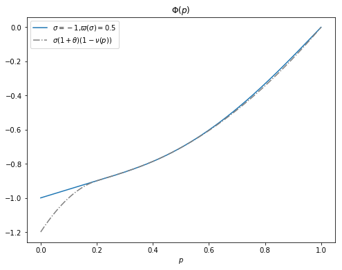

It can be seen from Figure 3 that is convex and different from when is near to 0 or 1. When is small, is linear which is due to the fact that is a good function. When is in the middle range, coincides with , which indicates that the derivative constraint is not likely tight, namely . This indeed can be observed from Figure 4. When is large, dominates , which corresponds to the tight case, namely . This can also be seen from Figure 4.
5 On the PO contracts
In this section we discuss some properties of the PO contracts.
5.1 PO contracts of deductible type
In this section we investigate under what conditions a deductible compensation is PO. Our first result reveals the classical assertion that all the PO contracts are of deductible type in the EU theory framework (see, e.g. [31]).
Proposition 5.1.
If there is no probability distortion, then all the PO contracts are of deductible type.
Proof.
Suppose there is no probability distortion, i.e., . Then (4.14) reduces to
| (5.1) |
Since is continuous and convex, is a continuous concave function on with boundary values and . Let
Then , on , and on . By (5.1), we obtain for . As is concave, there are two possible cases on :
- 1.
Either on , which trivially implies for .
- 2.
Or on , which by (5.1) also implies that for a.e. .
Therefore, in both cases, we have
By virtue of and (3.3), we obtain
Thanks to (3.12), we see the corresponding compensation
is of deductible type, where . In particular the compensation becomes the full coverage compensation if .
Remark 5.1.
When the probability weighting function is nontrivial, the following result answers the question completely by providing an equivalent condition.
Theorem 5.2.
The optimal solution to problem (2.7) corresponds to a deductible compensation with deductible if and only if
| (5.2) |
where
Moreover, the deductible satisfies .
Proof.
By (3.12), is the optimal solution to problem (2.7) if and only if
is the optimal solution to problem (3.10), which by Theorem 4.5 is also equivalent to
is a solution to (4.7) in . Thanks to (3.9), we have
By virtue of this, one can check is a solution to (4.7) holds true if and only if
But this is equivalent to (5.2) because
| (5.3) |
When , the condition (5.2) implies
The right hand side is clearly no more than 1, so .
Corollary 5.3.
If , then the full coverage compensation is not optimal for any RDU insured.
Proof.
By Theorem 5.2, we should have , so .
In particular, when has no mass at , namely , the condition in Corollary 5.3 is satisfied, therefore the full coverage compensation is not optimal for any RDU insured. On the other hand, by the proof of Proposition 5.1 and Remark 5.1, the full coverage compensation can be PO at least when and for . Therefore, the relative safety loading and the mass of at 0 play the critical role in determining the type of the PO contracts. Indeed, when the relative safety loading is small or has a large mass at 0, namely , the full coverage compensation can also be PO even if the probability weighting function is nontrivial. This will be shown in the following section.
Remark 5.2.
When , we have
Remark 5.3.
Clearly one can use our idea to find equivalent conditions for the optimal compensations being a special form such as the proportional coverage compensations. We leave this to the interested readers.
Remark 5.4.
Xu, Zhou and Zhuang [39] studied an optimal compensation problem, which is slight different from ours, but also under the RDU theory. Under certain assumptions (see Remark 2.2), they found that optimal compensation is of three-fold, that is
Their conditions are sufficient but not necessary, by our method, one can find the equivalent conditions for the above compensation being optimal to their problem.
When (5.2) is not satisfied, a PO contract may not be of deductible type. We are interested in which situation a moral-hazard-free contract is PO, that is, it is optimal for at least one RDU insured; in other words, economically speaking, when such a contract is acceptable in insurance market. This will be addressed in the following section.
5.2 When is a moral-hazard-free contract PO?
In this section, we consider the following reverse problem. For a given potential loss , a moral-hazard-free retention and a relative safety loading , is it possible to find at least one RDU insured such that the contract is optimal for her? Every RDU insured is characterized by her utility function , probability weighting function and wealth level . So the question can be mathematically stated as follows: for any given reasonable , can we find a triple such that is optimal to problem (2.7)?
When the relative safety loading is big or has a small mass at 0, namely , the answer is negative as we showed in Corollary 5.3 that it is impossible to find a RDU insured such that the full coverage contract is optimal for her. By contrast, when the relative safety loading is small or has a large mass at 0, namely , the following result gives an affirmative answer to the question.
Theorem 5.4.
Proof.
By Corollary 4.6, we only need to show that, for each good function , there exist infinite pairs such that is a solution to (4.14), where , and is the inverse function of .
Define
Since and , by continuity, we have and . Set any feasible on such that . By the definition of good function, we see is linear on . Since for , . Thus and for . By virtue of this,
So the ODE in (4.14) is satisfied for a.e. .
We now consider the problem on . Let
Since and , is absolutely continuous and strictly increasing. Moreover,
so . Because is continuous and non-decreasing and is strictly increasing on , there exists a utility function which is in with and such that
| the mapping is strictly increasing on . | (5.4) |
It then follows
Notice for , so
Because , the above equation implies the ODE in (4.14) is satisfied on . Since there are infinite many choices of that satisfies (5.4), the claim is proved.
Remark 5.5.
Remark 5.6.
The marginal case requires delicate analysis, we leave it to the interested readers.
6 PO contracts with non-monotone compensations or retentions
The incentive compatibility constraint is taken a priori into consideration in problem (2.6), so the PO contracts are free of ex ante moral hazard. One nature question is: what will the PO contracts look like if the incentive compatibility constraint is ignored in the problem formulation at beginning? We give complete answers to this question when the retentions or compensations are not necessary to be monotone. Since the analysis is similar to the case with incentive compatibility constraint, we just point out the main differences in the arguments and leave the details to the interest readers.
6.1 PO contracts with non-monotone compensations
If we only require the retentions to be monotone but put no constraint on the compensations, that is,
| (6.1) |
Then the corresponding set of compensations becomes
In this case the compensations in may not be monotone.
Theorem 6.1.
Proof.
The argument remains unchanged until (4.3). For any , since there is no upper bound limitation for in (6.1), so is for . Recall on , so the optimality condition (4.3) implies and
which can be equivalently expressed as
This leads to the following analog of (4.7),
By virtue of Lemma 4.4 and , the ODE in above can be rewritten as
It is easy to check and also satisfies the above ODE in place of . So is identical to on . In another words, with .
Remark 6.1.
Remark 6.2.
As we only have one side constraint for in this model, the related ODE becomes a single-obstacle problem. Furthermore, since the operator in the ODE is linear, we can solve it explicitly.
6.2 PO contracts with monotone retentions
If we only require the compensations to be monotone but put no constraint on the retentions, that is,
Then the corresponding set of retentions becomes
| (6.3) |
In this case the retentions in may not be non-decreasing.
Theorem 6.2.
If the set of retentions in problem (2.7) is replaced by (6.3), then a retention is optimal to problem (2.7) if and only if it can be written as
| (6.4) |
for some such that
| (6.5) |
Proof.
Remark 6.3.
Corollary 6.3.
If the probability weighting function is concave (such as no distortion case ), then the optimal retention given by (6.4) is moral-hazard-free.
Proof.
Remark 6.4.
The ODE (6.5) is still a single-obstacle problem as the previous model, but its operator is nonlinear in general so we cannot provide an explicit solution. When is an exponential utility, the operator, however, reduces to a linear one (see (4.11)). One can still show that after change of variable is the convex envelope of some known function. We encourage the interested reader to write down the details.
7 Concluding remarks
In this paper, we present a novel approach to computing all the PO moral-hazard-free insurance contracts under the RDU theory. Similar to [35, 37], the approach also works for problems under some other behavioral finance theories. For instance, one could use our method to consider the loss and gain parts in the cumulative prospect theory model, separately, and then combine them to get the optimal solution. Our method also allows us to find all the PO moral-hazard-free insurance contracts with general lower and/or upper bounds on the derivatives of the retentions and/or the compensations.
In our model, we considered the expected value premium principle for the insurer. It is possible to generalize our method to cope with models with other premium principles such as the variance premium principle and Wang’s premium principle for the insurer. In these cases, the problem becomes more challenging. We leave them for our future research.
Acknowledgments. The author is grateful to the Co-Editor Professor Jaksa Cvitanic and two anonymous referees for their constructive comments and suggestions which have helped to significantly improve the paper of the two previous versions, and to Mr. Jing Peng for help in calculating the numerical example in Section 4.2. The author is also grateful for comments from conference participants at The 12th AIMS Conference on Dynamical Systems, Differential Equations and Applications in Taipei, 2018 Conference in Memory of Professor Xunjing Li in Changchun, SCFM 2018 in Qingdao, 2018 International Conference on Mathematical Finance & Symposium on the Role of Mathematical Finance on FinTech Business in Daejeon, 2018 Stochastic Analysis, Stochastic Control and New Developments in Weihai, The 8th Annual Conference of Financial Engineering & Financial Risk Management Branch of OR Society of China in Xi’an, 2018 Advanced Methods in Mathematical Finance in Angers, The Sixth Asian Quantitative Finance Conference in Guangzhou, The First Conference on Actuarial Science and Applications in Shanghai.
References
- [1] Allais, M. (1953): Le comportement de l’homme rationnel devant le risque: critique des postulats et axiomes de l’ecole americaine, Econometrica, Vol. 21(4), pp. 503-546.
- [2] Arrow, K.J. (1963): Uncertainty and the welfare economics of medical care, The American Economic Review, Vol. 53(5), pp. 941-973.
- [3] Bernard, C., He, X.D., Yan, J.-A., and Zhou, X.Y. (2015): Optimal insurance design under rank-dependent expected utility, Mathematical Finance, Vol. 25, pp. 154-186.
- [4] Carlier, G., and Dana, R.-A. (2006): Law invariant concave utility functions and optimization problems with monotonicity and comonotonicity constraints, Statist. Decisions, Vol. 24(1), 127-152.
- [5] Carlier, G., and Dana, R.-A. (2008): Two-persons efficient risk-sharing and equilibria for concave law-invariant utilities, Economic Theory, Vol. 36(2), pp. 189-223.
- [6] Carlier, G., and Dana, R.-A. (2011): Optimal demand for contingent claims when agents have law invariant utilities, Mathematical Finance, Vol. 21(2), 169-201.
- [7] Chateauneuf, A., Dana, R.-A., and Tallon. J.-M. (2000): Optimal risk-sharing rules and equilibria with Choquet-expected-utility, Journal of Mathematical Economics, Vol. 34(2), pp. 191-214.
- [8] Dai, M., Xu, Z.Q., and Zhou, X.Y. (2010): Continuous–time Markowitz’s model with transaction costs, SIAM Journal on Financial Mathematics, Vol.1 (2010), 96-125.
- [9] Dai, M., and Yi, F.H. (2006): Finite-horizon optimal investment with transaction costs: A parabolic double obstacle problem, Journal of Differential Equations, Vol. 246(4), pp. 1445-1469.
- [10] Dana, R.-A., and Scarsini, M. (2007): Optimal risk sharing with background risk, Journal of Economic Theory, Vol. 133(1), pp. 152-176.
- [11] Ellsberg, D. (1961): Risk, ambiguity and the Savage axioms, Quarterly Journal of Economics, Vol. 75(4), pp. 643-669.
- [12] Friedman, M., and Savage, L.J. (1948): The utility analysis of choices involving risk, Journal of Political Economy, Vol. 56(4), pp. 279-304.
- [13] Ghossoub, M., (2019): Optimal insurance under rank-dependent expected utility, Insurance: Mathematics and Economics, Vol. 87, pp. 51-66.
- [14] Gollier, C., and Schlesinger, H. (1996): Arrow’s theorem on the optimality of deductibles: A stochastic dominance approach, Economic Theory, Vol. 7(2), pp. 359-363.
- [15] He, X. D., Jin, H., and Zhou, X. Y. (2015): Dynamic portfolio choice when risk is measured by Weighted VaR, Mathematics of Operations Research, Vol. 40(3), 773-796
- [16] He, X. D., and X. Y. Zhou (2011): Portfolio choice via quantiles, Mathematical Finance, Vol. 21, pp. 203-231.
- [17] Hou, D., and Z. Q. Xu (2016): A robust Markowitz mean–variance portfolio selection model with an intractable claim, SIAM Journal on Financial Mathematics, Vol.7, 124–151.
- [18] Huberman, G., Mayers, D., and Smith Jr, C.W. (1983): Optimal insurance policy indemnity schedules, The Bell Journal of Economics, Vol. 14(2), pp. 415-426.
- [19] Jin, H., S. Zhang, and X. Y. Zhou (2011): Behavioral portfolio selection with loss control, Acta Mathematica Sinica, Vol. 27, pp. 255-274.
- [20] Jin, H., and X. Y. Zhou (2008): Behavioral portfolio selection in continuous time, Mathematical Finance, Vol. 18, pp. 385-426
- [21] Kahneman, D., and A. Tversky (1979): Prospect theory: An analysis of decision under risk, Econometrica, Vol. 46, pp. 171-185
- [22] Lieberman, G.M. (1996): Second Order Parabolic Differential Equations, World Scientific.
- [23] Lopes, L. L. (1987): Between hope and fear: The psychology of risk, Advances in experimental social psychology, Vol. 20, pp.255-295
- [24] Mehra, R., and Prescott, E.C. (1985): The equity premium: A puzzle, Journal of Monetary Economics, Vol. 15(2), pp. 145-161
- [25] Picard, P. (2000): On the design of optimal insurance policies under manipulation of audit cost, International Economic Review, Vol. 41(4), pp. 1049-1071.
- [26] Prelec, D. (1998): The probability weighting function, Econometrica, Vol. 66, pp. 497-527
- [27] Quiggin (1982): A theory of anticipated utility, Journal of Economic and Behavioral Organization, Vol. 3(4), pp. 323-343
- [28] Raviv, A. (1979): The design of an optimal insurance policy, The American Economic Review, Vol. 69(1), pp. 84-96
- [29] Rüschendorf, L., and Vanduffel, S. (2020): On the construction of optimal payoffs, Decisions Econ Finan, Vol. 43, 129-153
- [30] Schied, A. (2004): On the Neyman–Pearson problem for law-invariant risk measures and robust utility functionals, Annals of Applied Probability, Vol. 14(3), 1398-1423
- [31] Spence, M., and Zeckhauser, R. (1971): Insurance, information, and individual action, The American Economic Review, Vol. 61, pp. 380-387
- [32] Tversky, A., and C. R. Fox (1995): Weighing risk and uncertainty, Psychological Review, Vol.102, pp. 269-283
- [33] Tversky, A., and D. Kahneman (1992): Advances in prospect theory: Cumulative representation of uncertainty, J. Risk Uncertainty, Vol. 5, pp. 297-323
- [34] Wei, P. (2018): Risk management with weighted VaR, Mathematical Finance, Vol. 28(4), 1020-1060
- [35] Xia, J. M., and X. Y. Zhou (2016): Arrow-Debreu equilibria for rank-dependent utilities, Mathematical Finance, Vol. 26, pp. 558-588
- [36] Xu, Z. Q. (2014): A new characterization of comonotonicity and its application in behavioral finance, J. Math. Anal. Appl., Vol. 418, pp. 612-625
- [37] Xu, Z. Q. (2016): A note on the quantile formulation, Mathematical Finance, Vol.26, No. 3, 589-601
- [38] Xu, Z. Q., and X. Y. Zhou (2013): Optimal stopping under probability distortion, Annals of Applied Probability, Vol. 23, pp. 251-282
- [39] Xu, Z. Q., X. Y. Zhou, and S. Zhuang (2019): Optimal insurance under rank-dependent utility and incentive compatibility, Mathematical Finance, Vol. 29(2), pp. 659-692
- [40] Yaari, M.E. (1987): The dual theory of choice under risk, Econometrica, Vol. 55(1), pp. 95-115