Self-reporting and screening: Data with current-status and censored observations

We study the estimation of failure time distribution where the failure times can be either observed directly, or be right-censored or left-censored. This type of survival data arises, for example, in estimation of time to the appearance of a medical condition where characteristic symptoms may or may not appear when the condition exists. Specific medical settings include relapse in childhood brain tumors, which may be observed due to clinical symptoms, or right-censored due to periodic screening with negative result (no tumor), or left-censored due to periodic screening with a positive result (Minn et al., 2001). Another medical setting is melanoma cancer, which is observed if self-detected, or is right censored due to a negative screening (no melanoma), or left-censored if it goes undetected until screening. Additional examples can be found in Whitehead (1989).

The motivating example for this work comes from estimating customer patience in service system which, as discussed by Mandelbaum and Zeltyn (2007), is a challenging problem. In our study, we focus on patients who wait for treatment in an emergency department (ED). Three categories of patients are observed. The first category consists of patients who get service and thus their patience time is right-censored by the waiting time. The second category comprises those who leave the system and announce it, and thus their patience time is observed while the waiting time is right-censored. The third category consists of patients who leave the system without announcing it; their absence is hence revealed only when they are called to service, which is after they have already left; formally, their patience time is left-censored.

Estimating the patience time is of importance as the decision of patients to leave the system before getting served might have a strong effect on their physical well-being. There has been considerable research on the reasons why patients leave an ED before being served; see Baker et al. (1991), Hunt et al. (2006), Bolandifar et al. (2014), and Batt and Terwiesch (2015). However, these and other authors have not proposed a model by which ED patience time - namely the duration that a potential patient is willing to wait for ED service - can be estimated, and this is our goal here.

We propose novel parametric and nonparametric estimators of the unknown survival function for this 3-type survival data. We then study their rates of convergence. The parametric estimator is based on both full and partial likelihoods. We provide condition under which the parametric estimator is a linear asymptotic normal (LAN) estimator and converges to a normal distribution in a root-$n$ rate. The nonparametric estimator is based on nonparametric kernel estimators for density functions and on a novel estimator of the cumulative probability function that has some similarities to the Nelson–Aalen estimator (e.g., Klein and Moeschberger, 2013, Chapter 4). We show that, under some regularity conditions, the nonparametric estimator point-wise converges to the normal distribution.

We perform a simulation study and compare the proposed parametric and nonparametric estimators. For the parametric model, we study both correct and misspecified models and show the different corresponding results. We show how the accuracy changes with sample size. We then carry out a case study that is based on data of patients waiting for treatment in an ED, in the U.S. in 2008. We analyzed separately different severity levels (15106 observations in the emergency group, 43600 in the urgent group, and 26541 in the semi-urgent group). We conclude with a comparison of the parametric and nonparametric estimators for the three different severity levels of this dataset.

Developing screening methods for medical conditions, such as breast and melanoma cancers, has a long history (Wilson et al., 1968; Zelen and Feinleib, 1969). In the classical setting, the medical condition either already exists at the time of screening and is thus left-censored, or does not exist, and is thus right-censored. The setting in which self-detection is possible, and thus the condition time is observed, has been surprisingly mostly ignored in the literature. For example, Minn et al. (2001) treat both self-detection times and screening times as event times, ignoring the censoring. The closest model to the one that we present here appears in Whitehead (1989). It is assumed there that the condition can be detected at screening or before screening due to symptoms. In both cases, the condition already exists at the time of detection. It is also assumed that screenings take place at a sequence of fixed time points. Whitehead (1989) recommends to ignore the extra knowledge gained due to self-reporting and to replace these times with the time of the next screening. The survival function is then estimated only at the discrete fixed screening times using standard techniques (Prentice and Gloeckler, 1978).

There has been considerable research effort, dedicated to modeling and analysis of customer (im)patience while waiting for service. Here we describe several papers that, together with references therein, provide what is required for a historical background and state-of-art perspective. First, we recommend the literature review (Section 3) in the recent Batt and Terwiesch (2015), accompanied by Gans et al. (2003): these survey patience-research from an operational/queueing view point (mainly Section 6.3.3 in the latter), while connecting it to the medical literature on LWBS (mainly Section 3 in the former); see also Aksin et al. (2007) who, relative to Gans et al. (2003), expand on managerial challenges. Next we mention Mandelbaum and Zeltyn (2013), which is an Explanatory Data Analysis of (im)patience in telephone call centers (that appears in a special issue that is devoted to models of queues abandonment). Finally, and the most related to the present study, are the following two studies. Brown et al. (2005) applies, in Section 5, the Kaplan–Meier estimator (Kaplan and Meier, 1958) to estimate the survival functions and consequently hazard rates, of both virtual waiting time and impatience; the data is that of a call center, in which times of abandonment are all recorded hence the data is right-censored. Then Wiler et al. (2013), which is also the source of our present ED data case study, estimate LWBS rates as a function of ED patient arrival rates, treatment times, and ED boarding times. There was no attempt in that work to estimate the patience-time distribution.

We conclude this brief survey with the observation that the estimation of customer (im)patience is relevant beyond screening, call centers, and EDs. For example, Nah (2004) studies tolerance of Web users (during information retrieval). Yom-Tov et al. (2018) analyzes chat services, in which customers abandon at any phase during chat-exchanges with a service center: one expects that such services give rise to the same options as in EDs: some customers receive service, others abandon without letting anyone know, and the rest announce their abandonment time.

In the standard setting of right-censored data one observes, for each patient, either the failure time or the censoring time. In terms of our motivating example, failure time is patience time while censoring time is the waiting time. Patience time is observed when patients leave the ED while informing the system of their departure; waiting time is observed when a patient is called for service. However, unlike in standard right-censored data and like in current status data, there are also patients who leave without informing; in this case their absence is observed only when they are called for service, and this latter time provides an upper bound for their patience time. In other words, the (virtual) waiting time is observed, and the only information on patience time is that it is less than this observed waiting time. Hence, in this case, the patience time is left-censored.

More formally, let $T$ be the patient’s failure time, i.e., the time until the patient loses patience. Let $W$ be the censoring time, i.e., the waiting time until the patient gets (or could have gotten) service. We assume that $T$ has a cumulative distribution function (cdf) $F$ and a probability density function (pdf) $f$, and that $W$ has cdf $G$ and pdf $g$. Let $\Delta$ be the indicator $\Delta\equiv 1{\{T<W\}}$; i.e., $\Delta=1$ if the patient loses patience before being called to service, and $\Delta=0$ otherwise.

Let $Y$ be the indicator that is $1$ for a patient who leaves and informs when leaving, and $0$ otherwise. Denote by $q(t)$ the conditional probability that a patient reports leaving given that the waiting time equals to $t$. In other words, $q(t)=pr(Y=1\mid{T=t})$. We assume that the waiting time $W$ and the patience time $T$ are independent. This assumption, which is common in the right-censored data literature (see, Klein and Moeschberger, 2013, Chapter 3, pages 65-66), seems appropriate in our case study, as we stratify by acuity levels. We also assume that announcement indicator $Y$ is independent of the waiting time $W$, as it seems reasonable that the decision of a patient to report when leaving does not depend on the waiting time. Summarizing, we assume that the pair $(Y,T)$ is independent of the waiting time $W$. When this assumption does not hold, different theoretical tools are needed for a valid estimation.

Let $U$ be the recorded time: $U\equiv{Y}{T}+(1-Y){W}$. The observed data consist of the triplets $(U_{i},Y_{i},\Delta_{i})$, $i=1,\ldots,n$, and there are three categories of patients:

$\mathcal{C}=1$:

The patient gets service, hence the waiting time is observed, which serves as a lower bound on the patience time; thus the patience time is right censored. Formally, $\Delta=0$, $Y=0$, and $U=W$.

$\mathcal{C}=2$:

The patient leaves without being treated and reports departure. The patience time is thus revealed: $Y=1$, $\Delta=1$, and $U=T$.

$\mathcal{C}=3$:

The patient leaves without reporting, hence virtual waiting time (the time that the patient would have waited had he stayed in the ED) is observed, which provides an upper bound for the patience time, thus the patience time is left-censored. Formally, $Y=0$, $\Delta=1$, and $U=W$.

See the proof in A.1.

For $i=1,2,3$, we introduce the following sub-stochastic distribution functions

From Lemma 1 above, we deduce that

Here, $\overline{F}(t)=1-F(t)$ and $\overline{G}(t)=1-G(t)$ are the survival functions of the patience time and the waiting time, respectively.

Define

Then $r_{i}$ is the density function of the observed time $U$ given $\mathcal{C}=i$. Our model assumes that all denominators are positive.

To summarise what is known and what is to be estimated, there are two unknown distributions in our setting, $G$ and $F$, and we aim to estimate them using both parametric and nonparametric techniques. For each patient, the waiting time is either observed or right censored. If the patient reports and then leaves, the waiting time is longer than the observed patience time. Hence, the waiting time is right-censored. Therefore, parametric and nonparametric estimation for the distribution of waiting time $W$ can be done by standard techniques for right-censored data. However, estimation of the distribution of patience time $T$, is more complicated and is discussed in Sections 4 and 5.

Assume now that the distributions of both the patience time and the waiting time belong to some parametric families. More formally, let $\mathcal{F}=\{f(\cdot;\theta),\theta\in\Theta\}$ where $\Theta\subseteq\mathbb{R}^{d}$, $\mathcal{G}=\{g(\cdot;\gamma),\gamma\in{\Gamma}\}$ where $\Gamma\subseteq\mathbb{R}^{p}$. We assume that the density of the patience time can be written as $f(t;\theta_{0})\in\mathcal{F}$. We also assume that the density of the waiting time can be written as $g(t;\gamma_{0})\in\mathcal{G}$. Write $h_{1}(t;\theta,\gamma)\equiv{g}(t;\gamma)\overline{F}(t;\theta)$, and similarly $h_{2}(t;\theta,\gamma)\equiv{q(t)}{f}(t;\theta)\overline{G}(t;\gamma)$ and $h_{3}(t;\theta,\gamma)\equiv{g}(t;\gamma)\int_{0}^{t}\left\{{}1-q(x)\right\}{}f(x;\theta)dx$.

The likelihood of the observed data $D=\{(U_{i},Y_{i},\Delta_{i}),i=1,\ldots,n\}$ can be written in terms of the functions $h_{1}$, $h_{2}$, and $h_{3}$, as follows:

Using the explicit representations of $h_{1}$, $h_{2}$, $h_{3}$, we obtain that $L(D;\theta,\gamma)$ is given by

The value of $\gamma$ that maximizes this likelihood is independent of $\theta$. Therefore, a maximum likelihood estimator (MLE) $\widehat{\gamma}_{n}$ to $\gamma_{0}$ can be constructed from this likelihood. However, maximizing the likelihood with respect to $\theta$ is difficult. Even if $\gamma$ is given or estimated, the maximizer of $\theta$ depends on the unknown function $q(t)$. Therefore, we consider the partial likelihood $L_{partial}(D;\theta;\gamma)$ of category $\mathcal{C}=1$,

The value of $\theta$ that maximizes this partial likelihood depends on $\gamma$. We plug the MLE $\widehat{\gamma}_{n}$ into this partial likelihood. In Theorem 1 below we show that, under standard regularity conditions, the maximizer $\widehat{\theta}_{n}$ of $L_{partial}(D;\theta;\widehat{\gamma}_{n})$ is a consistent and asymptotically normal estimator for $\theta_{0}$.

We need the following assumptions:

1. (A1)

   The derivative $\frac{\partial}{\partial{\theta}}{f(t;\theta)}$ is continuous in $t$ for each $\theta\in\Theta$, $\frac{\partial}{\partial{\gamma}}{g(t;\gamma)}$ is continuous in $t$ for each $\gamma\in\Gamma$.

2. (A2)

   For all $\theta\in\Theta$, $\arg\max_{\gamma\in\Gamma}{L(D;\theta,\gamma)}$ is unique, hence denote
   $\widehat{\gamma}(\theta)\equiv\arg\max_{\gamma\in\Gamma}{L(D;\theta,\gamma)}$. It is assumed as well that for each $\theta\in\Theta$, $\frac{\partial}{\partial\gamma}L\left\{D;\theta,\widehat{\gamma}(\theta)\right\}=0$.

3. (A3)

   For all $\gamma\in\Gamma$, $\arg\max_{\theta\in\Theta}{L_{partial}(D;\theta,\gamma)}$ is unique, hence denote
   $\widehat{\theta}(\gamma)\equiv\arg\max_{\theta\in\Theta}{L_{partial}(D;\theta,\gamma)}$. It is assumed as well that for each $\gamma\in\Gamma$, $\frac{\partial}{\partial\theta}L_{partial}\left\{D;\widehat{\theta}(\gamma),\gamma\right\}=0$.

The proof appears in Appendix A.1.

In this section we propose nonparametric estimators for the survival function of the patience time $\overline{F}$ and study its theoretical properties. For simplicity, we restrict the estimation to a segment $[0,\tau]$ for some $\tau>0$, such that the probability of $W$ and $T$ being larger than $\tau$ is positive. This is a standard condition in survival estimation (see Kosorok, 2008, Chapter 4.2). Note that for observations of Categories 1 and 3, the waiting-time is observed. For Category 2, only a lower bound of the waiting time is observed. Hence, the waiting time is either observed or right-censored. Therefore, estimating the waiting time distribution can be done by using standard survival analysis estimators such as the Kaplan–Meyer estimator (see Klein and Moeschberger, 2013, Chapter 4). On the other hand, estimating the distribution of the patience time is more challenging since we cannot distinguish between the density function $f$ and the unknown function $q$. Our goal is thus to estimate the distribution of the patience time F.

Assume that over all positive numbers, the waiting time density function $g$ is strictly positive. Recall that $h_{1}(t)=g(t)\overline{F}(t)$, $h_{3}(t)=g(t)\int_{0}^{t}{\left\{{}1-q(s)\right\}f(s)ds}$, where the functions $h_{1},h_{3}$ are defined as in (1). Therefore,

which is well defined as $g(t)>0$. Reordering the terms in (3), we get that

Hence,

From the definitions in (2), it follows that

Therefore, we propose to estimate F(t) by estimating the following terms:

(i) $pr(W\leq{T})$ and $pr(Y=0,T<W)$,

(ii) $r_{1}(t)$ and $r_{3}(t)$,

(iii) $A(t)\equiv\int_{0}^{t}{q(s)f(s)ds}$.

Estimating the expression in (i) can be done by the empirical estimators: $\widehat{pr}(T\leq{W})=n^{-1}\Sigma_{i=1}^{n}(1-\Delta_{i})$, $\widehat{pr}(Y=0,W<T)=n^{-1}\Sigma_{i=1}^{n}\Delta_{i}(1-Y_{i})$. These estimators converge, by the central limit theorem (CLT), to $pr(W\leq{T})$ and $pr(Y=0,T<W)$, respectively, at the rate of $n^{1/2}$.

Since $r_{1}$ and $r_{3}$ are density functions, they can be estimated using a kernel estimator (Tsybakov, 2008, Chapter 1.2). Let $\widehat{r}_{1}$ and $\widehat{r}_{3}$ be kernel estimators of $r_{1}$ and $r_{3}$, respectively. Assume that both $r_{1}$ and $r_{3}$ belong to a Sobolev function class of order $\beta$. Then for each $t>0$, both $\widehat{r}_{1}(t)$ and $\widehat{r}_{3}(t)$ converge at a rate of $n^{\beta/(2\beta+1)}$ (see Tsybakov, 2008, Chapter 1.7, for both the definition of a Sobolev class and the proof).

We now turn to estimate the term $A(t)={\int_{0}^{t}{q(s)f(s)ds}}$. A nonparametric estimator that we created for this term is defined and proven to be consistent in the following lemma.

The proof is given in Appendix A.3.

By plugging in the estimators

to the equation in (4), we get that

is an estimator of $F(t)$.

The proof appears in Appendix A.4.

We study the performance of both the parametric and nonparametric estimators that were proposed in Sections 4 and 5, respectively. Based on the setting of the case study discussed in Section 7, we consider two simulation settings. In the case study, both the exponential and Weibull distributions seem to fit well the waiting time and patience time distributions, respectively. The case study data also indicated that the mean of the waiting time $W$ is smaller then the patience time $T$. Thus, the two simulation settings consist of samples from exponential and Weibull distributions in which the waiting time has a smaller mean then the patience time mean. In the first setting, a sample was taken from the model in which the patience time $T$ follows an exponential distribution with rate $4$, and the waiting time $W$ follows an exponential distribution with rate $10$. In the second setting a sample was taken from a model in which the patience time $T$ follows a Weibull distribution with rate $4$ and shape $2$, and the waiting time $W$ follows an exponential distribution with rate $10$. In both settings, the unknown probability of announcement is $q(t)=\exp(-12t)$. Taking the probability of announcement to be the increasing function $q(t)=1-\exp(-12t)$ or the constant function $q(t)=0.5$ yields similar results which are omitted. Moreover, we experimented with additional numerical values. The behavior and conclusions, as reported here, remain consistent across these experiments.

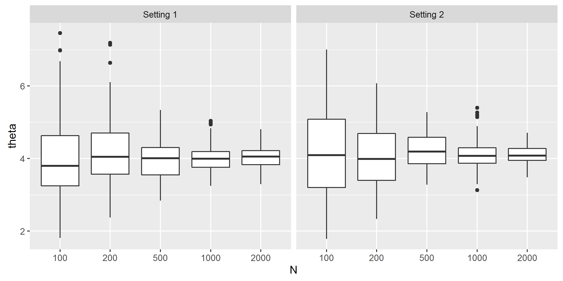
In each setting, we calculated the parametric estimator for the rate of $T$ for five different sample sizes ($N=100,200,500,1000,2000$). For each sample size, we repeated the simulation $100$ times. When using the parametric method, it was assumed that both $T$ and $W$ follow an exponential distribution with unknown parameters. Note that this assumption holds for the first setting but does not hold for the second one. In other words, the second setting is carried out under a misspecified model. The results are shown in Figure 1.

We compare $\widehat{\overline{F}}_{n}$, the estimator of the survival function of $T$, to the true survival function $\overline{F}_{0}$. For the parametric estimation, $\widehat{\overline{F}}_{n}(t)=\exp(-\hat{\theta}{t})$, while for the nonparametric estimator $\widehat{\overline{F}}_{n}(t)$ is given by (A.4). The comparison is done using mean square error (MSE), which is defined by

where $f_{0}$ is the density of $T$. The parametric and nonparametric survival function estimators are demonstrated in Figures 2 and 3. Figure 2 represents the results of the first setting in which $T\sim{Exp(4)}$ and $W\sim{Exp(10)}$. Figure 3 represents the results of the second setting in which $T\sim{Weibull(4,2)}$ and $W\sim{Exp(10)}$. Summaries of the MSE are given in Table 1. Not surprisingly, for Setting 1, since the parametric model is correct, the MSE is smaller for the parametric estimator. Similarly, since in Setting 2 the parametric model is incorrect, the MSE is smaller for the nonparametric estimator.

Retrospective data were collected from all patient presentations to triage at an urban, academic, adult-only emergency department (ED) with visits in calendar year 2008. This data was used for the analysis in Wiler et al. (2013). The data consist of the waiting time of patients arriving at emergency rooms. One of the categories defined in this data is acuity. Since our model assumes that all patients follow the same distribution, we calculated the estimators for each level of acuity separately. We focused on the following three levels of acuity: emergency, urgent, and semi-urgent. The emergency level consist of $15106$ patients, the urgent level consist of $43600$ patients, and the semi-urgent level consist of $26541$ patients.

The data consists of the triple variables $(U_{i},\Delta_{i},Y_{i})$ described in Section 3. At each acuity level, an observation is categorized to one of the three possible categories.

Parametric and nonparametric estimators for the survival of each acuity level were calculated. The results of these estimators are given in Figures 4 and 5. As can be seen in Figure 4, the nonparametric estimators of the patience time are stochastically ordered by levels of acuity. In other words, patients at the severe acuity level are less probable to loose patience than patients at the urgent level, who in turn are less prone to lose patience than patients at the semi-urgent level. The results for the parametric estimator seem unreasonable since one would expect that patients with more severe acuity level are more likely to loose patience, and loose it faster.

In this paper, we consider survival data that combine observed, right-censored, and left-censored data. The setting we analyzed was that of patients who wait for treatment in an emergency department, where some patients may leave without being seen. We proposed both parametric and nonparametric estimators for the distribution of the patience time. Using simulation, we showed that when the parametric model holds, the parametric estimator estimates the patience time well. However, when the model is misspecified, the nonparametric estimator behaved better. In our case study, we also observed that the nonparametric estimator performed better.

So far, no baseline covariates were given. Novel parametric and nonparametric estimators are needed for addressing settings that include baseline covariates.

Y. Ritov was partially supported by the Israeli Science Foundation (grant No. 1770/15).

Y. Goldberg was partially supported by the Israeli Science Foundation (grant No. 849/17).

References

- Aksin et al. [2007] Z. Aksin, M. Armony, and V. Mehrotra. The modern call center: A multi-disciplinary perspective on operations management research. Production and operations management, 16(6):665–688, 2007.
- Baker et al. [1991] D. W. Baker, C. D. Stevens, and R. H. Brook. Patients who leave a public hospital emergency department without being seen by a physician. Causes and consequences. JAMA, 266(8):1085–1090, 1991.
- Batt and Terwiesch [2015] R. J. Batt and C. Terwiesch. Waiting patiently: An empirical study of queue abandonment in an emergency department. Management Science, 61(1):39–59, 2015.
- Bolandifar et al. [2014] E. Bolandifar, N. DeHoratius, T. Olsen, and J. L. Wiler. Modeling the behavior of patients who leave the ED without being seen. Chicago Booth Research Paper, (12–14), 2014.
- Brown et al. [2005] L. Brown, N. Gans, A. Mandelbaum, A. Sakov, H. Shen, S. Zeltyn, and L. Zhao. Statistical analysis of a telephone call center: A queueing-science perspective. Journal of the American statistical association, 100(469):36–50, 2005.
- Gans et al. [2003] N. Gans, G. Koole, and A. Mandelbaum. Telephone call centers: Tutorial, review, and research prospects. Manufacturing & Service Operations Management, 5(2):79–141, 2003.
- Hunt et al. [2006] K. A. Hunt, E. J. Weber, J. A. Showstack, D. C. Colby, and M. L. Callaham. Characteristics of frequent users of emergency departments. Annals of Emergency Medicine, 48(1):1–8, 2006.
- Kaplan and Meier [1958] Edward L Kaplan and Paul Meier. Nonparametric estimation from incomplete observations. Journal of the American statistical association, 53(282):457–481, 1958.
- Klein and Moeschberger [2013] J. P. Klein and M. L. Moeschberger. Survival Analysis: Techniques for Censored and Truncated Data. Springer, New York, 2013.
- Kosorok [2008] M. R. Kosorok. Introduction to Empirical Processes and Semiparametric Inference. Springer, New York, 2008.
- Mandelbaum and Zeltyn [2007] A. Mandelbaum and S. Zeltyn. Service engineering in action: The Palm/Erlang-A queue, with applications to call centers. In Advances in Services Innovations, D. Spath and K. P. Fahnrich (eds.). Springer, New York,, pages 17–45, 2007.
- Mandelbaum and Zeltyn [2013] A. Mandelbaum and S. Zeltyn. Data-stories about (im) patient customers in tele-queues. Queueing Systems, 75(2-4):115–146, 2013.
- Minn et al. [2001] A Yuriko Minn, Brad H Pollock, Linda Garzarella, Gary V Dahl, Larry E Kun, Jonathan M Ducore, Atsuko Shibata, James Kepner, and Paul G Fisher. Surveillance neuroimaging to detect relapse in childhood brain tumors: a pediatric oncology group study. Journal of clinical oncology, 19(21):4135–4140, 2001.
- Nah [2004] F. Nah. A study on tolerable waiting time: how long are web users willing to wait? Behaviour & Information Technology, 23(3):153–163, 2004.
- Prentice and Gloeckler [1978] Ross L Prentice and Lynn A Gloeckler. Regression analysis of grouped survival data with application to breast cancer data. Biometrics, pages 57–67, 1978.
- Tsybakov [2008] A. B. Tsybakov. Introduction to Nonparametric Estimation. Springer Science & Business Media, New York, 2008.
- van der Vaart [2000] A. W. van der Vaart. Asymptotic Statistics. Cambridge University Press, Cambridge, 2000.
- Whitehead [1989] John Whitehead. The analysis of relapse clinical trials, with application to a comparison of two ulcer treatments. Statistics in medicine, 8(12):1439–1454, 1989.
- Wiler et al. [2013] J. L. Wiler, E. Bolandifar, R. T. Griffey, R. F. Poirier, and T. Olsen. An emergency department patient flow model based on queueing theory principles. Academic Emergency Medicine, 20(9):939–946, 2013.
- Wilson et al. [1968] James Maxwell Glover Wilson, Gunnar Jungner, World Health Organization, et al. Principles and practice of screening for disease. 1968.
- Yom-Tov et al. [2018] G. B. Yom-Tov, A. Rafaeli, S. Ashtar, D. Altman, M. Westphal, M. Natapov, and N. Barkay. Customer emotion in chat services: Automatic identification and new insights. Under review, 2018.
- Zelen and Feinleib [1969] Marvin Zelen and Manning Feinleib. On the theory of screening for chronic diseases. Biometrika, 56(3):601–614, 1969.