Thermodynamics of Restricted Boltzmann Machines and Related Learning Dynamics
Abstract
We investigate the thermodynamic properties of a Restricted Boltzmann Machine (RBM), a simple energy-based generative model used in the context of unsupervised learning. Assuming the information content of this model to be mainly reflected by the spectral properties of its weight matrix , we try to make a realistic analysis by averaging over an appropriate statistical ensemble of RBMs.
First, a phase diagram is derived. Otherwise similar to that of the Sherrington-Kirkpatrick (SK) model with ferromagnetic couplings, the RBM’s phase diagram presents a ferromagnetic phase which may or may not be of compositional type depending on the kurtosis of the distribution of the components of the singular vectors of .
Subsequently, the learning dynamics of the RBM is studied in the thermodynamic limit. A “typical” learning trajectory is shown to solve an effective dynamical equation, based on the aforementioned ensemble average and explicitly involving order parameters obtained from the thermodynamic analysis. In particular, this let us show how the evolution of the dominant singular values of , and thus of the unstable modes, is driven by the input data. At the beginning of the training, in which the RBM is found to operate in the linear regime, the unstable modes reflect the dominant covariance modes of the data. In the non-linear regime, instead, the selected modes interact and eventually impose a matching of the order parameters to their empirical counterparts estimated from the data.
Finally, we illustrate our considerations by performing experiments on both artificial and real data, showing in particular how the RBM operates in the ferromagnetic compositional phase.
1 Introduction
The Restricted Boltzmann Machine (RBM) [1] is an important machine learning tool used in many applications, by virtue of its ability to model complex probability distributions. It is a neural network which serves as a generative model, in the sense that it is able to approximate the probability distribution corresponding to the empirical distribution of any set of high-dimensional data points living in a discrete or real space of dimension . From the theoretical point of view, the RBM is of high interest as it is one of the simplest neural network generative models and the probability distribution that it defines presents a simple analytic form. Moreover, there are clear connections between RBMs and well known disordered systems in statistical physics. As an example, when data are composed by vectors with binary components the discrete RBM takes the form of an heterogeneous Ising model composed of one layer of visible units (the observable variables) connected to one layer of hidden units (the latent or hidden variables building up the dependencies between the visible ones), in which couplings and fields are obtained from the training data through a learning procedure. In order to build more powerful models, RBMs can be stacked to form “deep” architectures. In such a case, they can form a multi-layer generative model known as a Deep Boltzmann Machine (DBM) [2] or they can be stacked and trained layerwise as a pre-training procedure for neural networks [3]. The standard learning algorithms in use are the contrastive divergence [4] (CD) and the refined Persistence CD [5] (PCD), which are based on a quick Monte Carlo estimation of the response function of the RBM and are efficient and well documented [6]. Nevertheless, despite some interesting interpretations of CD in terms of non-equilibrium statistical physics [7], the learning of RBMs remains a set of obscure recipes from the statistical physics point of view: hyperparameters (like the size of the hidden layer) are supposed to be set empirically without any theoretical guidelines.
Historically, statistical physics played a central role in studying the theoretical foundations of neural networks. In particular, during the 1980s many works on the Hopfield model [8, 9, 10, 11] managed to define its learning capacity and to compute the number of independent patterns that it could store. It is worth noticing that, as RBMs are ultimately defined as a Boltzmann distribution with pairwise interactions on a bipartite graph, they can be studied in a way similar to that used for the Hopfield model. The analogy is even stronger since connections between the Hopfield model and RBMs have been made explicit when using Gaussian hidden variables [12], here the number of patterns of the Hopfield model corresponding to the number of hidden units. Motivated by a renewed excitement for neural networks, recent works actually propose to exploit the statistical physics formulation of the RBM to understand what is its learning capacity and how mean-field methods can be exploited to improve the model. In [13, 14, 15], mean-field based learning methods using TAP equations are developed. TAP solutions are usually expected to define a decomposition of the measure in terms of pure thermodynamical states and are useful both as an algorithm to compute the marginals of the variables of the model and to identify the pure states when they are yet unknown. For instance, in a sparse explicit Boltzmann machine (i.e. without latent variables) this implicit clustering can be done by means of belief propagation fixed points 11 1 a somewhat different form of the TAP equations with simple empirical learning rules [16]. In [17, 18], an analysis of the static properties of RBMs is done assuming a given weight matrix , in order to understand collective phenomena in the latent representation, i.e. the way latent variables organize themselves in a compositional phase [19, 20] to represent actual data. These analysis make use of the replica trick (or equivalent) making the common assumption that the components of the weight matrix are i.i.d.; despite the fact that this approach may give some insights into the retrieval phase, this approximation is problematic since, as far as a realistic RBM is concerned (an RBM learned on data), the learning mechanism introduces correlations within the weights of and then it seems rather crude to continue to assume the independence and hope to understand the realistic statistical properties of the model.
Concerning the learning procedure of neural networks, many recent statistical physics based analyses have been proposed, most of them within teacher-student setting [21]. This imposes a rather strong assumption on the data in the sense that it is assumed that these are generated from a model belonging to the parametric family of interest, hiding as a consequence the role played by the data themselves in the procedure. From the analysis of related linear models [22, 23], it is already a well established fact that a selection of the most important modes of the singular values decomposition (SVD) of the data is performed in the linear case. In fact in the simpler context of linear feed-forward models the learning dynamics can be fully characterized by means of the SVD of the data matrix [24], showing in particular the emergence of each mode by order of importance with respect to the corresponding singular values.
First steps to follow this guideline have been done in [25], in the context of a general RBM and to address the shortcomings of previous analyses, in particular concerning the assumptions over the weights distribution. To this end it has been proposed to characterize both the learned RBM and the learning process itself by means of the SVD spectrum of the weight matrix in order to single out the information content of the RBM. It is assumed that the SVD spectrum is split in a continuous bulk of singular vectors corresponding to noise and a set of outliers that represent the information content. By doing this it is possible to go beyond the usual unrealistic assumption of i.i.d. weights made for analyzing RBMs. Proceeding along this direction, in the present work we first present a thermodynamic analysis of RBMs under the more realistic assumptions over the weight matrix that we propose. Then, on the same basis, the learning dynamics of RBMs is studied by direct analysis of the dynamics of the SVD modes, both in the linear and non-linear regimes.
The paper is organized as follows: in Section 2 we introduce the RBM model and its associated learning procedures. Section 3 presents the static thermodynamical properties of the RBM with realistic hypothesis on its weights: a statistical ensemble of weight matrices is discussed in Section 3.1; mean-field equations in the replica-symmetric (RS) framework are given in Section 3.2 and the corresponding phase diagram is studied in Section 3.3 with a proper delimitation of the RS domain where the learning procedure is supposed to take place. The ferromagnetic phase is studied in great details in 3.4 by looking in particular at the conditions leading to a compositional phase. Section 4 is devoted to the learning dynamics. In Section 4.1, a deterministic learning equation is derived in the thermodynamic limit and a set of dynamical parameters is shown to emerge naturally from the SVD of the weight matrix. This equation is analyzed for linear RBMs in Section 4.2 in order to identify the unstable deformation modes of that result in the first emerging patterns at the beginning of the learning process; the non-linear regime is described in Section 4.3, on the basis of the thermodynamic analysis, by numerically solving the effective learning equations in simple cases. Our analysis is finally illustrated and validated in Section 5 by actual tests on the MNIST dataset.
2 The RBM and its associated learning procedure
An RBM is a Markov random field with pairwise interactions defined on a bipartite graph formed by two layers of non-interacting variables: the visible nodes and the hidden nodes representing respectively data configurations and latent representations (see Figure 1). The former noted correspond to explicit representations of the data while the latter noted are there to build arbitrary dependencies among the visible units. They play the role of an interacting field among visible nodes. Usually the nodes are binary-valued (of Boolean type or Bernoulli distributed) but Gaussian distributions or more broadly arbitrary distributions on real-valued bounded support are also used [26], ultimately making RBMs adapted to more heterogeneous data sets. Here to simplify we assume that visible and hidden nodes will be taken as binary variables (using values gives the advantage of working with symmetric equations hence avoiding to deal with the “hidden” biases on the variables that appear when considering binary variables). Like in the Hopfield model [8], which can actually be cast into an RBM [12], an energy function is defined for a configuration of nodes
| (1) |
and this is exploited to define a joint distribution between visible and hidden units, namely the Boltzmann distribution
| (2) |
where is the weight matrix and and are biases, or external fields on the variables. is the partition function of the system. The joint distribution between visible variables is then obtained by summing over hidden ones. In this context, learning the parameters of the RBM means that, given a dataset of samples composed of variables, we ought to infer values to , and such that new generated data obtained by sampling this distribution should be similar to the input data. The general method to infer the parameters is to maximize the log likelihood of the model, where the pdf (2) has first been summed over the hidden variables
| (3) |
Different learning methods have been set up and proven to work efficiently, in particular the contrastive divergence (CD) algorithm from Hinton [4] and more recently TAP based learning [13]. They all correspond to expressing the gradient ascent on the likelihood as
| (4) | ||||
| (5) | ||||
| (6) |
where is the learning rate. The main problem are the terms on the right hand side of (4-6). These are not tractable and the various methods basically differ in their way of estimating those terms (Monte-Carlo Markov chains, naive mean-field, TAP…). For an efficient learning the terms must also be approximated by making use of random mini-batches of data at each step.
3 Static thermodynamical properties of an RBM
3.1 Statistical ensemble of RBMs
When analyzing the thermodynamical properties of RBMs, it is common to assume that the weights are i.i.d. random variables, like for example in [20, 17, 18]. This generally leads to a Marchenko-Pastur (MP) distribution [27] of the singular values of , which is unrealistic.
In order to clarify our notation, let us recall the definition of the singular value decomposition (SVD). As a generalization of eigenmodes decomposition to rectangular matrices, the SVD for a RBM is given by
| (7) |
where is an orthogonal matrix whose columns are the left singular vectors , is an orthogonal matrix whose columns are the right singular vectors and is a diagonal matrix whose elements are the singular values . The separation into left and right singular vectors is due to the rectangular nature of the decomposed matrix, and the similarity with eigenmodes decomposition is revealed by the following SVD equations
In [25] it is argued that the MP distribution of SVD modes actually corresponds to the noise of the weight matrix, while the information content of the RBM is better expressed by the presence of SVD modes outside of this bulk. This leads us to write the weight matrix as
| (8) |
where the are isolated singular values (describing a rank matrix), the and are the dominant eigenvectors of the SVD decomposition and the are i.i.d. terms corresponding to noise, with . The and are two sets of respectively and -dimensional orthonormal vectors, which means that their components are respectively and , and . We assume to be the rank of and and for all . Note that in the limit and with fixed and , has a spectrum density composed of a Marchenko-Pastur bulk of eigenvalues and of set of discrete modes:
with
The interpretation for the noise term is given by the presence of an extensive number of modes at the bottom of the spectrum, along which the variables won’t be able to condense but that still contribute to the fluctuations. In the present form our model of RBM is similar to the Hopfield model and recent generalizations [28], the patterns being represented by the SVD modes outside of the bulk. The main difference, in addition to the bipartite structure of the graph, is the non-degeneracy of the singular values . The choice made here is to consider finite, giving which means that the thresholds (having the meaning of feature detectors) should be because feature is detected when an extensive number of spins is aligned with . In addition, this allows us to assume simple distributions for the components of and (for instance, considering them i.i.d.). Altogether, this defines the statistical ensemble of RBM to which we restrict our analysis of the learning procedure.
Another approach would be to consider extensive, thereby assuming that all modes can potentially condense even though they are associated to dominated singular values. In that case, the separation between the condensed modes and the rest should be made when order parameters are introduced and the noise would then correspond to uncondensed modes. If the number of condensed modes is assumed to be extensive, then we should instead consider an average over the orthogonal group which would lead to a slightly different mean-field theory [29, 30].
3.2 Replica symmetric Mean-field equation
Our analysis in the thermodynamic limit follows classical treatments using replicas, like [31, 9] for the Hopfield model or [17] for bipartite models. The starting point is to express the average over and of the log partition function in (2) with the help of the replica trick:
First the average over yields
After this averaging, 4 sets of order parameters and are introduced with the help of two distinct Hubbard-Stratonovich transformations. The first one corresponds to
The second one is aimed at extracting magnetization’s contributions correlated with the modes:
with
| (9) |
These variables represent the following quantities:
namely the correlations of the hidden [resp. visible] states with the left [resp. right] singular vectors and the Edward-Anderson (EA) order parameters measuring the correlation between replicas of hidden or visible states. and denote an average w.r.t. the rescaled components and of the SVD modes. The transformations involve pairs of complex integration variables because of the asymmetry introduced by the two-layers structure in contrast to fully connected models.
We obtain the following representation:
with and
| (10) | ||||
| (11) |
with
Since is an incomplete basis we also need to take care of the potential residual transverse parts and , such that the following decompositions hold:
| (13) | ||||
| (14) |
To keep things tractable, both and will be considered negligible in the sequel. Taking into account these components would lead to the addition of a random field to the effective RS field of the variables and eventually to a richer set of saddle point solutions. Note that the order of magnitude of and is at this stage an assumption. If and (or and ) were uncorrelated they would scale as . Moreover, regarding the ensemble average, we will consider and fixed in the sequel.
The thermodynamic properties are obtained by first making a saddle point approximation possible by letting first and taking the limit afterwards. We restrict here the discussion to RS saddle points [32]. The breakdown of RS can actually be determined by computing the so-called AT line [33] (see Appendix A). At this point we assume a non-broken replica symmetry. The set reduces then to a pair of spin glass parameters, i.e. and for all , while quenched magnetizations on the SVD directions are now represented by .
Taking the limit yields the following limit for the free energy:
| (15) |
Assuming a replica-symmetric phase, the saddle-point equations are given by
| (16) | ||||
| (17) |
where
and , with and denoting an average over the Gaussian variable and the rescaled components and of the SVD modes. We note that the equations are symmetric under the exchange , simultaneously with , and , given that and have the same distribution. In addition, for independently distributed and and vanishing fields (), solutions corresponding to non-degenerate magnetizations have symmetric counterparts: each pair of non-vanishing magnetizations can be negated independently as , generating new solutions. So to one solution presenting condensed modes, there correspond distinct solutions.
3.3 Phase Diagram
The fixed point equations (16, 17) can be solved numerically to tell us how the variables condensate on the SVD modes within each equilibrium state of the distribution and whether a spin-glass or a ferromagnetic phase is present. The important point here is that with finite and a non-degenerate spectrum the mode with highest singular value dominates the ferromagnetic phase.
In absence of bias () and once is interpreted as temperature and as ferromagnetic couplings, we get a phase diagram similar to that of the Sherrington-Kirkpatrick (SK) model with three distinct phases (see Figure 2)
- •
a paramagnetic phase () (P),
- •
a ferromagnetic phase () (F),
- •
a spin glass phase (; ) (SG).
In general, the lines separating the different phases correspond to second order phase transitions and can be obtained by a stability analysis of the Hessian of the free energy. They are related to unstable modes of the linearized mean-field equations and correspond to an eigenvalue of the Hessian becoming negative.
The (SG-P) line is obtained by looking at the Hessian in the sector:
from what results that the spin glass phase develops when 22 2 Note that in [17] a dependence is found. This dependence is hidden in our definition of giving times the variance of instead of as in their case.. This transition line is understood tacking directly into account the spectral properties of the weight matrix. Classically, this is done with the help of the linearized TAP equations and exploiting the Marchenko-Pastur distribution [32]. In our context, the linearized TAP equations read
given the variance of the weights in absence of dominant modes. Then we can show that the paramagnetic phase becomes unstable when the highest eigenvalue of the matrix on the rhs is equal to : if is a singular value of , the corresponding eigenvalues verify the relation
from which it is clear that the largest eigenvalue corresponds to the largest singular value . Owing to the Marchenko-Pastur distribution so verifies
is readily obtained for .
For the (F-SG) frontier we can look at the sector corresponding to the emergence of a single mode (written in the spin-glass phase):
From this it is clear that the first mode to become unstable is the mode with highest singular value and this occurs when and , solutions of (16,17), verify
As for the SK model, this line appears to be well below the de Almeida-Thouless (AT) line, which is the line above which the RS solution is stable (see Figure 2, and Appendix A for the computation of the AT line). This means that in principle a replica symmetry breaking treatment would be necessary to properly separate the two phases. However, we will leave aside this point as we are mainly interested in the practical aspects, namely the ability of the RBM to learn arbitrary data, and so we are mostly concerned with the ferromagnetic phase above the AT line.
For the (P-F) line we consider the same sector of the Hessian but now written in the paramagnetic phase, i.e. setting in the above equation, and this simply yields the emergence of the single mode for .
Note that all of this is independent on how the statistical average over and is performed. Instead, as we shall see later on, the way of averaging influences the nature of the ferromagnetic phase.
Regarding the stability of the RS solution, the computation of the AT line reported in Appendix A is similar to the classical one made for the SK model, though slightly more involved. In fact we were not able to fully characterize, in replica space, all the possible instabilities of the Hessian which would potentially lead to a breakdown of the replica symmetry. At least the one responsible for the ordinary SK model RS breakdown has a counterpart in the bipartite case that gives a necessary condition for the stability of the RS solution:
For the terms below the radical become identical and the condition reduces to the one of the SK model, except for the averages which are not present in the SK model. In Figure 2, is shown the influence on the phase diagram of the value of and of the type of average made on and .
3.4 Nature of the Ferromagnetic phase
Some subtleties arise when considering various ways of averaging over the components of the singular vectors. In [19, 20] is emphasized the importance for networks to be able to reproduce compositional states structured by combination of hidden variables. In our representation, we don’t have direct access to this property but, in some sense, to the dual one, which is given by states corresponding to combinations of modes. Their presence and their structure are rather sensitive to the way the average over and is performed. In this respect the case in which and have i.i.d. Gaussian components is very special: all fixed points associated to dominated modes can be shown to be unstable and fixed points associated to combinations of modes are not allowed. To see this, first notice that in such a case the magnetization’s part of the saddle point equations (16,17) read
| (18) | ||||
| (19) |
Since the role of the bias is mainly to introduce some asymmetry between otherwise degenerated fixed points obtained by sign reversal of at least one pair , let us analyze the situation without fields, i.e. by setting . We immediately see that as long as the singular values are non degenerate, only one single mode may condense at a time. Indeed if mode condenses we necessarily have
and this can be verified only by one mode at a time. Looking at the stability of the fixed points, we see that only the fixed point associated to the largest singular value is actually stable (details reported after the introduction of lemma 3.1).
For other distributions like uniform Bernoulli or Laplace, instead, stable fixed points associated to many different single modes or combinations of modes can exist and contribute to the thermodynamics. In order to analyze this question in more general terms we first rewrite the mean-field equations in a convenient way which require some preliminary remarks. We restrict the discussion to i.i.d. variables so that we can consider single variable distributions. Joint distributions will be distinguished from single variable distributions by the use of bold: , being the (finite) number of modes susceptible of condensing.
Given the distribution and assuming it to be even, we define a related distribution attached to mode :
| (20) |
This distribution has some useful properties.
Lemma 3.1.
Given that is centered with unit variance and kurtosis , is a centered probability distribution with variance
Proof.
Consider the moments of . For odd they vanish while for even they read:
i.e. the even moments of relate to moments of order of . The lemma then follows from the fact that has unit variance.
In this respect, the Gaussian averaging is special because we have and . Then the mean-field equations (16,17) corresponding to the magnetizations can be rewritten in a form similar to (18,19) by introducing the variables and :
| (21) | ||||
| (22) |
with
| (23) | ||||
| (24) |
where
This rewriting will prove very useful also in the next section when analyzing the learning dynamics.
Let us now assume, in absence of bias, a non-degenerate fixed point associated to some given mode with finite and . The fixed point equation imposes the relation
| (25) |
The stability of such a fixed point with respect to any other mode is related to the positive definiteness of the following block of the Hessian
with, in the present case
This reduces to
Therefore for the Gaussian averaging case, since , and given (25), we necessarily have
i.e. the Hessian has negative eigenvalues. This means that if the mode is dominated by another mode , the magnetization will develop until , while will vanish.
For the general case of i.i.d. variables, assuming and obey the same distribution , let and be the cumulative distributions associated respectively to and
Given the values of obtained from the fixed point associated to mode , we have the following property:
Proposition 3.2.
If
which in turn implies
with
Proof.
In other words if dominates on then there is a positive stability gap defined as
| (26) |
such that there is a non-empty range for higher values of for which the fixed point associated to mode corresponds to a local minimum of the free energy. Note that property (i) [resp. (ii)] is analogous (in the sense that it implies it) to having a larger [resp. smaller] variance than , i.e. [resp. ]. Therefore distributions with negative relative kurtosis () will tend to favor the presence of metastable states, while the situation will tend to be more complex for probabilities with positive relative kurtosis. Indeed, in the latter case the fixed point associated to the highest mode might not correspond to a stable state if lower modes in the range are present, and fixed points associated to combinations of modes have to be considered. Note that in contrary with the Gaussian case, this can happen because is different for each mode and therefore more flexibility is offered by equations (21,22) than from equations (18,19).
Let us give some examples. Denote by the relative kurtosis. As already said the Gaussian distribution is a special case with . In addition, for instance for corresponding to Bernoulli, Uniform or Laplace, we have the following properties illustrated in the inset of Figure 2:
- •
Bernoulli ():
then for , yielding a positive stability gap.
- •
Uniform ():
It can be verified that for , yielding again a positive stability gap.
- •
Laplace ():
Here we have for , yielding a negative stability gap.
These three examples fall either in condition (i) or (ii), with a stability gap that is either always positive or always negative, independently of . We can also provide examples for which the stability condition may vary with . Consider for instance a sparse Bernoulli distribution, with a sparsity parameter:
The relative kurtosis is in this case
Looking at and it is seen that both conditions and are not fulfilled, except for which corresponds to the plain Bernoulli case. As we see in the inset of Figure 2, for the stability gap is always negative, meaning that a unimodal ferromagnetic phase is not stable, and it is replaced by a compositional ferromagnetic phase at all temperatures. Instead, for and at sufficiently high temperature (low ) the single mode fixed point dominate the ferromagnetic phase.
Laplace distribution:
let us look at the properties of the phase diagram in the case of singular vectors’ components being Laplace i.i.d., case in which a negative stability gap is expected and it may lead to a compositional phase. For this we need the expression for a sum of Laplace variables to compute the averages involved in (16,17). For this purpose, we define the following distributions:
Their Laplace transform upon decomposing into partial fractions reads:
and
where
From these decompositions we immediately identify
This results in the following decomposition of the EA parameters:
| (27) | ||||
| (28) | ||||
| (29) |
with
and
This allows for an efficient resolution of the mean-field equations (16,17,21,22), which let us observe the appearance of a purely compositional phase in the ferromagnetic domain when the modes at the top of the spectrum get close enough. In order to characterize this phase, we consider the stability gap for which the range lies below the highest mode , such that the ferromagnetic states correspond to the condensation of distinct modes present in this interval, including the highest.
In addition, this will prove useful when analyzing the learning dynamics described in the next section.
4 Learning dynamics of the RBM
4.1 Learning dynamics in the thermodynamic limit
A mean field analysis of the learning dynamics has been proposed in [25], in the form of phenomenological equations obtained after averaging over some parameters of the RBM, i.e. by choosing a well defined statistical ensemble of RBMs and using self-averaging properties in the thermodynamic limit. Here we rederive these equations, we add some details and then explore their properties in the light of the preceding section. First we project the gradient ascent equations (4-6) onto the bases and defined by the SVD of . Discarding stochastic fluctuations usually inherent to the learning procedure and letting the learning rate , the continuous version of (4-6) can be recast as follows:
| (30) | ||||
| (31) | ||||
| (32) |
with and given in (9). We also have
where
By eliminating , and we get the following set of dynamical equations:
| (33) | ||||
| (34) | ||||
| (35) |
along with the infinitesimal rotation generators of the left and right singular vectors
| (36) | ||||
| (37) |
where
The dynamics of learning is now expressed in the reference frame defined by the singular vectors of . The skew-symmetric rotation generators of the basis vectors (induced by the dynamics) tell us how data rotate relatively to this frame. Given the initial conditions, these help us keeping track of the representation of data in this frame. Note that these equations become singular when some degeneracy occurs in because then the SVD is not uniquely defined. Except from the numerical point of view, where some regularizations might be needed, this does not constitute an issue. In fact only rotations among non-degenerate modes are meaningful, while the rest corresponds to gauge degrees of freedom.
At this point our set of dynamical equations (33-37) is written in a general form. Our goal is to find the typical trajectory of the RBM within a certain statistical ensemble. For this reason, we make the hypothesis that the learning dynamics is represented by a trajectory in the space , while the specific realization of , and in (8) can be considered irrelevant and only the way they are distributed is important. We are then allowed to perform an average over , and with respect to some simple distributions, as long as this average is correlated with the data. By this we mean that the components of any given sample are kept fixed while averaging. In the end, what really matters are the strength and the rotation of the SVD modes, respectively determined by and . As a simplification and also by lack of understanding of what intrinsically drives their evolution, the distributions of and will be considered stationary in the sequel. Concerning , we allow its variance to vary with time in order to give a minimal description of how the MP bulk evolves during the learning. The detailed dynamics of will be derived later in Section 4.3.
Using the same notation of Section 3.4 and in particular using the rescaling , the empirical terms take the form:
| (38) | ||||
| (39) |
where
Note that the last equation actually depends on the activation function (hyperbolic tangent in this case), and the term corresponds to and is obtained by central limit theorem from the independence of the . is the empirical counterpart of the EA parameters and already encountered in Section 3.4, and for simple i.i.d. distributions like Gaussian or Laplace it can be estimated easily. The main point here is that the empirical terms (38,39) define operators whose decomposition over the SVD modes of functionally depends only on and on the projection of the data over the SVD modes of . These terms are driving the dynamics in a precise way. The adaptation of the RBM to this driving force is given by the terms in (33,34,35), which can be estimated in the thermodynamic limit (see Section 4.3) as a function of , and alone, by means of the order parameters given in Section 3.2 and once the mean-field equations (16,17) have been solved. Of course, all of this is based on the hypothesis that the RBM stays in the RS domain during learning. Experimental evidence supports this hypothesis (see Section 5).
4.2 Linear instabilities
At the beginning of the learning, the elements of the weight matrix are usually small; therefore, we can analyze the linear behavior of the RBM in order to understand what happens. In particular, we will see that the dynamics of a non-linear RBM at the beginning of the learning can be understood by looking at the stability analysis of the learning process. The purpose of this analysis is to identify which “deformation modes” of the weight matrix are the most unstable, and how they are related to the input data. Additionally, a good feature of the linear case is that no averaging is needed, the dynamics being actually independent on the particular realization of the components and . Also, always relative to the linear case, no distinction has to be made between dominant modes and other modes to be treated as the noise component of equation (8), we can simply put all of the modes on the same footing.
Let us analyze the linear regime for an RBM with binary units. The derivation is done by rescaling all the weights and fields by a common “inverse temperature” and letting this go to zero in equation (4). In principle, the stability analysis would lead to assume both the weights and the magnetizations to be small. However, we can assume only the magnetizations to be small and consider a slightly more general case with no approximations. Such a case is analogous to a linear RBM whose magnetizations undergo Gaussian fluctuations, and it is derived by keeping up to quadratic terms of the magnetizations in the mean field free energy:
where the variances of respectively visible and hidden variables read ():
| (40) | ||||
| (41) |
We omitted the quadratic term in coming from the TAP contribution to the free energy, which is optional for our stability analysis. In absence of this term the modes evolve strictly independently, while taking it into account leads to a correction to individual variances which couples the modes.
Magnetizations of visible and hidden variables have now Gaussian fluctuations with covariance matrix
We can discard the biases of the data and the related fields ( with a proper centering of the variables, and we consider equation (33) directly involving the covariance matrix of the data expressed in the frame defined by the SVD modes of
From we get the other terms yielding the following equations:
Note that these equations are exact for a linear RBM, since they can be derived without any reference to the coordinates of and over which we average in the non-linear regime. These equations tell us that the learning dynamics drives the rotation of the vectors (and ) until they are aligned to the principal components of the data, i.e. until becomes diagonal. Calling the empirical variance of the data, the system reaches the following equilibrium values:
assuming fixed. From this we see that the RBM selects the strongest SVD modes of the data. The linear instabilities correspond to directions along which the variance of the data is above the threshold , and they determine the development of the unstable deformation modes of the weight matrix; during the learning process, these modes will eventually interact following the usual mechanism of non-linear pattern formation encountered for instance in reaction-diffusion processes [34]. Other possible deformations are damped to zero. The linear RBM will therefore learn all the principal components that passed the threshold (up to ). Note that this selection mechanism is already known to occur for linear auto-encoders [23] or other similar linear Boltzmann machines [22]. On Fig. 3 we can see the eigenvalues being learned one by one in a linear RBM.
If we take into account the expressions (40,41) for , we see that the system cannot reach a stable solution except for the case in which all the modes are below the threshold at the beginning. Otherwise the modes that are excited first will eventually grow like for a large time, and the excitation threshold will tend to zero for all modes.
In any case, by the definition of a multivariate Gaussian, this simple non-linear analysis describes a unimodal distribution. In order to properly understand the dynamics and the steady-state regime of a non-linear RBM, a well suited mean-field theory is required.

4.3 Non-linear regime
In the linear regime, some specific modes are selected and at some point they start to interact in a non-trivial manner. As seen explicitly in (39), the empirical terms in (4-6) involve higher order statistics of the data and then the Gaussian estimation with of the RBM response terms and is no longer valid when the interactions kick in. Schematically, the linear regime is valid as long as the RBM is found in the paramagnetic phase. But as soon as one mode passes the linear threshold, the system enters the ferromagnetic phase. Then the proper estimation of the response terms follows from the thermodynamic analysis performed in Section 3, and depends on the assumptions made on the statistical properties of the components of the singular vectors of the weight matrix. In the case of Gaussian i.i.d. components, given the analysis proposed in Section 3.4, we know that the mode with the highest singular value completely dominates the ferromagnetic phase: we expect one single ferromagnetic state characterized by magnetizations aligned to this mode only, while magnetizations correlated to other modes vanish. To be precise, this is the correct picture without fields () but we don’t expect this picture to drastically change in the case of non-vanishing fields. In fact, solving the mean-field equations in presence of the fields show the appearance of meta-stable states correlated with single dominated modes; however, the free energy difference with respect to the ground state, i.e. the state correlated with the mode with the highest singular value, is of order , which means that the contribution of those meta-stable states become rapidly negligible with large system size.
To draw a realistic picture of the learning process we now consider Laplace i.i.d. components for the SVD modes that, as seen in Section 3.4, allow the ferromagnetic phase to be of compositional type. The reason for this is that the Laplace distribution leads to less interference among modes than the Gaussian distribution, so that the modes will weakly interact in the mean-field equations. Solving equations (21,22,27,29) in absence of fields yields the following picture: one fixed point solution will typically have non-vanishing magnetizations for all such that , where is approximately the gap defined in (26). This solution is a degenerate ground state, all other solutions being obtained by independently reversing the signs of the condensed magnetizations . Hence for condensed modes we get a degeneracy of . When the fields are included, all these fixed points are displaced in the direction of the fields, and some of them may disappear. In the end we are left with a potentially large amount of nearly degenerate states able to cover the empirical distribution of the data, at least in some simple cases.

Coming back to the learning dynamics the terms corresponding to the response of the RBM in (4,6) are estimated in the thermodynamic limit by means of the previously defined order parameters:
Here denotes the thermodynamical average and the partition function is expressed, in the thermodynamic limit, as
The index runs over all the stable fixed point solutions of (16,17) weighted accordingly to the free energy given by (15). These are the dominant contributions as long as free energy differences are , and the internal fluctuations given by each fixed point are comparatively of order . In addition, the dynamics of the bulk can be characterized by empirically defining :
whose evolution is:
given the independence of (resp. ) and (resp. ).
Exploiting the self-averaging properties of both the empirical and the response terms with respect to , and yields
with
Summarizing, our equations take the suggestive form
| (42) | ||||
| (43) | ||||
| (44) | ||||
| (45) |
with taking the form of a difference between a data averaging and a thermodynamical averaging involving only order parameters. Note here that the variables, with respect to the other variables, evolve on a faster time scale. This is our final and main result, which might possibly help improving current learning algorithms of RBMs. From this, it is clear what the learning of an RBM is aimed at: the equations will converge once the dataset is clustered in such a way that each cluster is represented by a solution of the mean-field equations with magnetizations and EA parameters corresponding respectively to their empirical counterparts and representing cluster magnetization and variance. In particular, these clusters can somehow be regarded as the attractors in the context of feed-forward networks, defining a partition of the data. This can be seen by starting from random configurations and letting the system evolve using the TAP equations or a MCMC method. At the end the system will end up in one of those clusters (characterized by a fixed point of the mean-field equations). Note that this is the reason why the RBM needs to reach a ferromagnetic phase with many states to be able to match the empirical term in (4) and reach convergence.
Additionally, the log likelihood (3) can be estimated in the thermodynamic limit (after normalization by ).
As an example, for a multimodal data distribution with a finite number of clusters embedded in a high dimensional configuration space, the SVD modes of that will develop are the one pointing to the directions of the magnetizations defined by these clusters (which will be almost surely orthogonal, given the high dimensionality of the embedding space). In this simple case the RBM will evolve, as in the linear case, to a state in which the empirical term becomes diagonal, while the singular values will adjust to match the proper magnetization in each fixed point.
We have integrated equations (42,43,44,45,36,37) in simple cases by using the Laplace averaging of the components of the SVD modes and using for the EA parameters the expressions given in (27,29). Basically, the hidden distribution to be modeled is defined by
| (46) |
i.e. a multimodal distribution composed of clusters of independent variables, where the magnetization of each variable in cluster is given by . Each cluster is weighted by some probability . In addition we assume these magnetization vectors to be embedded in a low dimensional space of dimension . defines the rank of . The initial conditions for are such that the left singular vectors span this low dimensional space. An example of the typical dynamics obtained in the case at hand is shown in Figure 4. In contrast to the linear problem where singular values evolve independently, here we distinctively witness the interaction between singular values: a kind of pressure is exerted by lower modes on higher ones resulting in successive bumps in the dynamics of the top modes. The number of states is roughly multiplied by two each time a mode condenses and get close enough to the top modes. Concerning the dynamics of the fields, we don’t really observe convergence towards stable directions. Some (possibly numerical) instability is observed when many modes condense, with both the fields and the number of fixed point solutions becoming very noisy. It is also interesting to see how the magnetizations related to the states are distributed with respect to the dataset. On Figure 5 we see that the fixed points tend (as expected) to settle within dense regions of sample points. However, our coarse description shows some limitations for more complex situations, the number of adjustable parameters being too limited to be able to match arbitrary distributions of clusters. It is then appropriate to think about this behaviour in a mean sense; at least, it is able to reproduce a realistic learning dynamics of the singular values of the weight matrix.
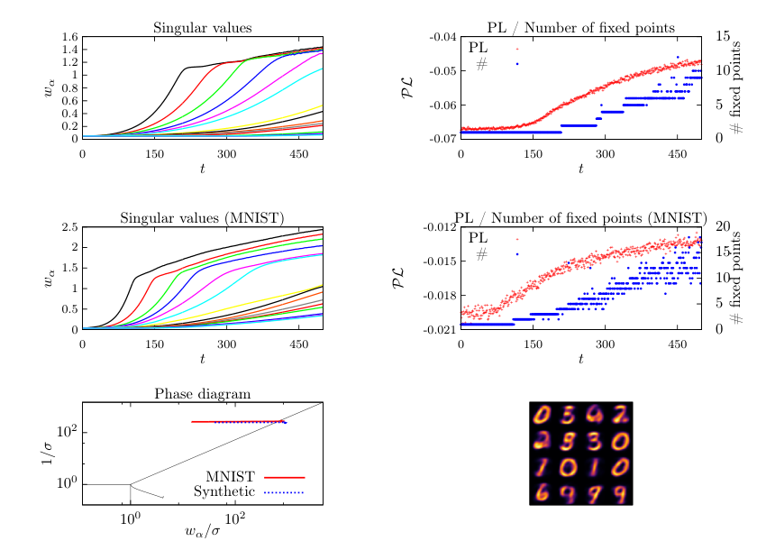
5 Numerical Experiments
Given the comprehensive theoretical analysis of the RBM model given in the previous sections, we are now able to provide a meaningful description of the learning dynamics for a RBM trained with k-steps contrastive divergence (CDk) [4]. The observations presented in this section will serve as a validation for the theoretical analysis. First, to provide a more direct comparison to section 4.3, we will look at the learning dynamics of an RBM trained on a set of simple synthetic data. Subsequently, we will test the model against real world data by training on the MNIST dataset.
5.1 Synthetic dataset
As a simple case, we trained the RBM over the same dataset defined in fig. 4, derived from the simple multimodal distribution in eq. 46 (see Appendix B for details). Thus we set , and we trained using samples with an effective dimension organized in separate clusters. The weights are initialized from a Gaussian distribution with standard deviation , while the hidden bias is initialized to and the visible bias is initialized with the empirical mean of the data
where is the empirical probability of activation for the hidden node.
Finally, the training set is divided into batches of size , 5 Gibbs sampling steps are used (CD5) and the learning rate is kept low in order to reduce noise, . The results of the analysis are shown in fig. 6. We see that the dynamics of the singular values obtained by direct integration of the mean-field equations (Fig. 4) are very well reproduced, the only difference being a slightly higher pressure on the strongest modes. The number of fixed point solutions also seems to follow the same trend but more noise is present, an indication of the fact that the RBM has a tendency to learn spurious fixed points during the training. The learning trajectory on the phase diagram is also of interest; we see that the RBM is initialized in the paramagnetic state as expected and the effect of the learning is to drive the model to the ferromagnetic phase. Once in the ferromagnetic phase, the trajectory slows down and the model is assessed near the critical line between paramagnetic and ferromagnetic states, where the estimate of the weights is most stable (according to [35]). Finally, in Fig. 8 we see how the RBM is able to generate a proper clustering of the data over the spectral modes. In particular, the TAP fixed points of the trained model are well distributed and able to cover the full data distribution, improving over the typical behaviour for Laplace distributed weights that emerged with our theoretical analysis (Fig. 5).

5.2 MNIST dataset
The MNIST dataset is composed by 70000 handwritten digits (60000 for training, 10000 for testing) of size pixels. Being highly multimodal, we expect this dataset to push the limits of our spectral analysis. For the training, the initialization of the model is the same one used for the synthetic data, 10000 training samples are used (taken at random from the dataset) and the values of the other hyperparameters are as follows: , , batch size , . With respect to the linear regime (described in section 4.2) we see in Fig. 9 how the RBM is able to learn the SVD of the dataset quite precisely at the beginning of the training, then the learning dynamics quickly enter the non-linear regime. Even in this highly multimodal scenario, our findings over simple synthetic data seem to be confirmed, as seen in Fig. 6. The high number of modes, however, determines an increase in the magnitude of the singular values of condensed modes and seems to destabilize a bit the learning, making the computation of fixed points less reliable. In fact, as a high number of modes are condensing, the model is not able to get rid of all the spurious fixed points. This problem can be mitigated by using an even smaller learning rate, at the cost of slowing down the training. Probably, using a variable learning rate could be a more practical solution (descreasing the learning rate from time to time to let the model eliminate unneeded fixed points). Concerning the (relative) kurtosis of the mode components distributions, we did not observe a very stable and systematic behavior. Either we see small fluctuations around zero, either some excursions occur and a finite value in the range is building up either for the or the components, coherently to the compositional phase interpretation given previously. The latter is the case for MNIST, as shown in Fig. 7. Additionally the transverse part of the fields, meaning orthogonal to the condensed modes, is usually not completely negligible, in contrary to what we assume in (13,14). This clearly constitutes a limitation of our analysis. These transverse components offer more flexibility for generating and selecting fixed points and interfere in some non-trivial way with the kurtosis property, which possibly explains why we don’t get a systematic behavior.


6 Discussion
Before drawing some perspectives, let us summarize the main outcomes of the present work:
- •
(i) thermodynamic properties of realistic RBMs: our analysis focused on a non-i.i.d. ensemble of weight matrices, whose derivation has been inspired by empirical observations obtained by training RBMs on real data.
- •
(ii) RS equations and compositional phase: we found a way of writing the RS equations for the RBM (in particular with equations (21,22,23,24)) which leads to a simple characterization of the ferromagnetic phase where the RBM is assumed to operate. Schematically, a negative relative kurtosis for the distribution of the singular vectors’ components favors the proliferation of metastable states, while a positive one tends to favor a compositional phase. In particular, we were able to precisely address a concrete case presenting the compositional phase by considering a Laplace distribution for the singular vectors’ components.
- •
(iii) a set of equations representing a typical learning dynamics that defines a trajectory in . The spectrum of the dominant singular values, represented by and expressing the information content of the RBM, is playing the main role. The bulk of dominated modes corresponding to noise sees its dynamics summarized by the evolution of . Rotations of dominant singular vectors during the learning process are given by while the projections of the biases along the main modes are given by and . These equations have been obtained by averaging over the components of left and right SVD vectors of the weight matrix, while keeping fixed the quantities considered to be relevant. This averaging actually corresponds to a standard self-averaging assumption in a RS phase.
- •
(iv) a clustering interpretation of the training process is obtained through equations (42,43,44,45) where it is explicitly shown the kind of matching that the RBM is trying to perform between the order parameters obtained from the fixed point solutions and their empirical counterparts in the non-linear regime. A natural clustering of the data can actually be defined by assigning to each sample the fixed point obtained after initializing the fixed point equations with a visible configuration corresponding to that same sample.
The main picture emerging from the present analysis is that of a set of clusters corresponding to the fixed points of the RBM, which try to uniformly cover the support of the dataset. A full understanding of the mechanism by which the RBM manages to properly cover the dataset is still lacking, even though the case of Laplace distributed singular vectors’ components gives some insights. By comparison, real RBMs have more flexibility than the simple “mean Laplace RBM” considered in Section 3.4 and they can produce a good covering of the data manifold. We were not yet able to precisely pinpoint the main ingredients for that mechanism, even though we suspect the transverse biases (orthogonal to the modes) of the hidden units to be the missing ingredient in our analysis.
From the theoretical point of view we would like to see how these results can be adapted to more complex models like DBM or generative models based on convolutional networks. In particular we would like to understand whether adding more layers can facilitate the covering of the dataset by fixed points. From the practical point of view these results might help to orientate the choice of the hyper-parameters used for training an RBM and to refine the criteria for assessing the quality of a learned RBM. For instance, the choice of the number of hidden variables is dictated by two considerations: the effective rank of , i.e. the number of relevant modes to be considered, and the level of interaction between these modes. Using less hidden variables gives more compact RBMs and reduces the rank of to its needed value, but it also leads to modes with stronger interactions, which means less flexibility for generating a good covering of fixed points.
Appendix A AT line
The stability of the RS solution to the mean-field equations is studied along the lines of [33] by looking at the Hessian of the replicated version of the free energy and identifying eigenmodes from symmetry arguments. Before taking the limit the free energy reads
with and given in (10,11). Assuming the small perturbations
around the saddle point , the perturbed free energy reads
where means “conjugate term” in the sense , …, where and the operators are given by
with
Conjugate quantities are obtained by replacing by , by , by , by and by . As for the SK model, the Hessian thereby defined can be diagonalized with the help of three similar sets of eigenmodes corresponding to different permutation symmetries in replica space.
The first set corresponds to replica symmetric modes defined by and solving the linear system
with eigenvalue solving a polynomial equation of degree corresponding to a vanishing determinant in the above system.
The second set corresponds to a broken replica symmetry where one replica is different from the others
This set has dimension . Its parameterization is obtained by imposing orthogonality with the previous one. The corresponding system reads
Finally the eigenmodes of the Hessian are made complete by considering a broken symmetry where two replicas and are different from the others, with the following parameterization dictated again by orthogonality constraints with the previous sets:
The dimension of this set is now , and it represents eigenvectors iff the following system of equations is satisfied
The corresponding eigenvalues read
with degeneracy . Finally the RS stability condition reads
which reduces to the same form of the AT line for the SK model when , except for the and averages that are specific to our model. As seen in Figure 2 the influence of is very limited.
Appendix B Synthetic dataset
The multimodal distribution modeling the N-dimensional synthetic data is
| (47) |
where is the number of clusters, is a weight and is a hidden field for cluster . The values for are taken at random and normalized, while to compute we take into account the magnetizations . Expanding over the spectral modes, we can set an effective dimension by constraining the sum to the range
| (48) |
Clusters’ magnetizations are drawn at random between and normalized with the factor
| (49) |
where is introduced to decrease the clusters’ polarizations (in our simulations, we used ). The spectral basis is obtained by drawing at random N-dimensional vectors and applying the Gram-Schmidt process (which can be safely employed as N is supposedly big and thus the initial vectors are nearly orthogonal). The hidden fields are then obtained from the magnetizations
| (50) |
and the samples are generated by choosing a cluster according to and setting the visible variables to according to
| (51) |
References
- [1] P. Smolensky. In Parallel Distributed Processing: Volume 1 by D. Rumelhart and J. McLelland, chapter 6: Information Processing in Dynamical Systems: Foundations of Harmony Theory. 194-281. MIT Press, 1986.
- [2] R. Salakhutdinov and G. Hinton. Deep Boltzmann machines. In Artificial Intelligence and Statistics, pages 448–455, 2009.
- [3] G.E. Hinton and R.R. Salakhutdinov. Reducing the dimensionality of data with neural networks. Science, 313(5786):504–507, 2006.
- [4] G. E. Hinton. Training products of experts by minimizing contrastive divergence. Neural computation, 14:1771–1800, 2002.
- [5] T. Tieleman. Training restricted Boltzmann machines using approximations to the likelihood gradient. In Proceedings of the 25th International Conference on Machine Learning, ICML ’08, pages 1064–1071, New York, NY, USA, 2008. ACM.
- [6] G.E. Hinton. A Practical Guide to Training Restricted Boltzmann Machines, pages 599–619. Springer Berlin Heidelberg, Berlin, Heidelberg, 2012.
- [7] D.S.P. Salazar. Nonequilibrium thermodynamics of restricted Boltzmann machines. Phys. Rev. E, 96:022131, 2017.
- [8] J. J. Hopfield. Neural networks and physical systems with emergent collective computational abilities. Proceedings of the National Academy of Sciences of the United States of America, 79(8):2554–2558, 1982.
- [9] D. J. Amit, H. Gutfreund, and H. Sompolinsky. Statistical mechanics of neural networks near saturation. Annals of Physics, 173(1):30–67, 1987.
- [10] E. Gardner. Maximum storage capacity in neural networks. EPL (Europhysics Letters), 4(4):481, 1987.
- [11] E. Gardner and B. Derrida. Optimal storage properties of neural network models. Journal of Physics A: Mathematical and General, 21(1):271, 1988.
- [12] B. Barra, A. Bernacchia, E. Santucci, and P. Contucci. On the equivalence of Hopfield networks and Boltzmann machines. Neural Networks, 34:1–9, 2012.
- [13] G. Marylou, E.W. Tramel, and F. Krzakala. Training restricted Boltzmann machines via the Thouless-Anderson-Palmer free energy. In Proceedings of the 28th International Conference on Neural Information Processing Systems, NIPS’15, pages 640–648, 2015.
- [14] H. Huang and T. Toyoizumi. Advanced mean-field theory of the restricted Boltzmann machine. Physical Review E, 91(5):050101, 2015.
- [15] C. Takahashi and M. Yasuda. Mean-field inference in gaussian restricted Boltzmann machine. Journal of the Physical Society of Japan, 85(3):034001, 2016.
- [16] C. Furtlehner, J.-M. Lasgouttes, and A. Auger. Learning multiple belief propagation fixed points for real time inference. Physica A: Statistical Mechanics and its Applications, 389(1):149–163, 2010.
- [17] A. Barra, G. Genovese, P. Sollich, and D. Tantari. Phase diagram of restricted Boltzmann machines and generalized Hopfield networks with arbitrary priors. arXiv:1702.05882, 2017.
- [18] H. Huang. Statistical mechanics of unsupervised feature learning in a restricted Boltzmann machine with binary synapses. Journal of Statistical Mechanics: Theory and Experiment, 2017(5):053302, 2017.
- [19] E. Agliari, A. Barra, A. Galluzzi, F. Guerra, and F. Moauro. Multitasking associative networks. Phys. Rev. Lett., 109:268101, 2012.
- [20] R. Monasson and J. Tubiana. Emergence of compositional representations in restricted Boltzmann machines. Phys. Rev. Let., 118:138301, 2017.
- [21] L. Zdeborová and F. Krzakala. Statistical physics of inference: thresholds and algorithms. Advances in Physics, 65(5):453–552, 2016.
- [22] M. E. Tipping and C. M. Bishop. Mixtures of probabilistic principal component analyzers. Neural Comput., 11(2):443–482, 1999.
- [23] H. Bourlard and Y. Kamp. Auto-association by multilayer perceptrons and singular value decomposition. Biological Cybernetics, 59(4):291–294, 1988.
- [24] A. M. Saxe, J. L. McClelland, and S. Ganguli. Exact solutions to the nonlinear dynamics of learning in deep linear neural networks. arXiv:1312.6120, 2014.
- [25] A. Decelle, G. Fissore, and C. Furtlehner. Spectral dynamics of learning in restricted Boltzmann machines. EPL, 119(6):60001, 2017.
- [26] E.W. Tramel, M. Gabrié, A. Manoel, F. Caltagirone, and F. Krzakala. A Deterministic and Generalized Framework for Unsupervised Learning with Restricted Boltzmann Machines. arXiv:1702.03260, 2017.
- [27] V. A. Marčenko and L. A. Pastur. Distribution of eigenvalues for some sets of random matrices. Mathematics of the USSR-Sbornik, 1(4):457, 1967.
- [28] M. Mézard. Mean-field message-passing equations in the Hopfield model and its generalizations. Phys. Rev. E, 95:022117, 2017.
- [29] G. Parisi and M. Potters. Mean-field equations for spin models with orthogonal interaction matrices. Journal of Physics A: Mathematical and General, 28(18):5267, 1995.
- [30] M. Opper and O. Winther. Adaptive and self-averaging Thouless-Anderson-Palmer mean field theory for probabilistic modeling. Physical Review E, 64:056131, 2001.
- [31] D. J. Amit, H. Gutfreund, and H. Sompolinsky. Spin-glass models of neural networks. Phys. Rev. A, 32:1007–1018, 1985.
- [32] M. Mézard, G. Parisi, and M. A. Virasoro. Spin Glass Theory and Beyond. World Scientific, Singapore, 1987.
- [33] J. R. L. Almeida and D. J. Thouless. Stability of the Sherrington-Kirkpatrick solution of a spin glass model. J.Phy. A:Math. Gen, 11(5):983–990, 1978.
- [34] P. C. Hohenberg and M. C. Cross. An introduction to pattern formation in nonequilibrium systems, pages 55–92. Springer Berlin Heidelberg, Berlin, Heidelberg, 1987.
- [35] I. Mastromatteo and M. Marsili. On the criticality of inferred models. Journal of Statistical Mechanics: Theory and Experiment, 2011(10):P10012, 2011.