Designer Spatial Control of Interactions in Ultracold Gases

Tunability of interactions in ultracold atomic gases has been achieved by exploiting magnetically controlled collisional (Feshbach) resonances [1], where the total energy of two colliding atoms in an energetically open channel is tuned into resonance with a bound dimer state in a closed channel. Optical field control offers a much richer palate, by creating designer interactions with high resolution in position, energy, momentum, and time. These techniques enable new paradigms. For example, energy resolution will provide better models of neutron matter by controlling the effective range [2, 6], while momentum resolution will permit non-zero momentum pairing in two component Fermi gases, i.e., synthetic FFLO states [4, 5]. The increased temporal resolution enables studies of non-equilibrium thermodynamics of strongly interacting gases on time scales faster than the Fermi time [6]. Spatial manipulation of interactions can be utilized to study controllable soliton emission [7], exotic quantum phases [8], long-living Bloch oscillations of matter waves [9], the physics of Hawking radiation from black holes [10], and scale-invariant dimer pairing [11]. However, optical techniques generally suffer from atom loss and heating due to spontaneous scattering, which severely limits their applicability [12, 13, 14, 15, 16, 17, 18, 19, 20].

In a major breakthrough for suppressing spontaneous scattering, Bauer et al., [18] used a bound-to-bound transition in the closed channel, which is far away from the atomic resonance. To further suppress atom loss, large detunings on the bound-bound transition were employed. The large detunings limited the tunability of the scattering length $a$ to $\Delta a\simeq 2\,a_{bg}$, where $a_{bg}$ is the background scattering length. In addition, interactions were tuned by changing the intensity of the laser light, which changes the net external potential experienced by the atoms. Recently, Clark and coworkers [20] avoided this problem by using a “magic” wavelength, tuned in between $D1$ and $D2$ lines of ¹³⁷Cs atoms, to suppress the atomic polarizability and hence the change in the external potential, but achieved a tunability of only $\simeq 0.2\,a_{bg}$. Further, this technique cannot be adopted universally, as it leads to excessive atom loss in atomic species such as ⁶Li, where the $D1$ and $D2$ lines are closely spaced.

Recently, we demonstrated new two-field optical techniques [2, 6], employing EIT [21] in the closed channel to control magnetic Feshbach resonances [1, 23], Fig. 1a. Our technique [1] tunes the scattering length near a two-photon resonance, where the loss is at a minimum and tunability of scattering length is at a maximum, in contrast to single-field optical methods [18, 20], where the maximum tunability in the scattering length is associated with maximum loss. Further, our method employs frequency tuning of a few MHz (small compared to the detuning $\approx 1.5$ THz from the atomic resonance), rather than intensity tuning, producing a negligible change in the net external potential experienced by the atoms. This eliminates the need for a “magic” wavelength [20] and makes our method universally applicable.

Here we report optical tuning of the scattering length in ⁶Li up to $\Delta a\simeq 12\,a_{bg}$, where $a_{bg}=62\,a_{0}$, with $a_{0}$ the bohr radius. Exploiting this wide tunability, we demonstrate spatial control of interactions by creating an interaction “sandwich”, where the central region of the atomic cloud is resonantly interacting $\Delta a>10\,a_{bg}$ and is surrounded by two weakly interacting regions $\Delta a\simeq 1\,a_{bg}$.

The basic level scheme of our technique is shown in Fig 1a. Optical fields $\nu_{1}$ (Rabi frequency $\Omega_{1}$ and detuning $\Delta_{1}$) and $\nu_{2}$ (Rabi frequency $\Omega_{1}$ and detuning $\Delta_{2}$), couple the ground molecular states of the singlet potential, $|g_{1}\rangle$ and $|g_{2}\rangle$, to the excited state $|e\rangle$, tuning the energy of $|g_{1}\rangle$ with suppressed optical scattering. The lowest two hyperfine states in ⁶Li, $|1\rangle$ and $|2\rangle$, have an energy-dependent narrow Feshbach resonance (width $\Delta B=0.1$ G) at $B_{res}=543.27$ G [24], where the atoms are predominantly in the spin triplet state $|T,k\rangle$, which tunes downward with magnetic field $B$ as $-2\mu_{B}\,B$, where $\mu_{B}\,$ is the Bohr magneton. The triplet continuum $|T,k\rangle$ is coupled to state $|g_{1}\rangle$ with a second order hyperfine coupling constant $V_{HF}$, which causes the narrow Feshbach resonance. For our experiments, we use $\Omega_{1}=0.5\,\gamma_{e}$, $\Omega_{2}=2.2\,\gamma_{e}$, where $\gamma_{e}=2\pi\times 11.8$ MHz is the decay rate of the excited molecular state and $\Delta_{1}=+\,2\pi\times 19$ MHz. We define the two-photon detuning $\delta=\Delta_{2}-\Delta_{1}$, which is varied by changing the frequency of the $\nu_{2}$ laser and holding the frequency of $\nu_{1}$ laser constant. $\delta\equiv 0$ is the two-photon resonance corresponding to minimum loss. For $\delta\equiv 0$, the state $|g_{1}\rangle$ also returns to its original unshifted position. The state $|g_{1}\rangle$ is below (above) its unshifted position for $\delta<0$ ($\delta>0$).

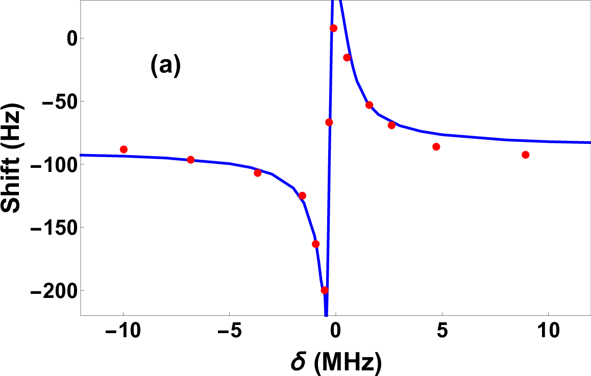
We first use radio frequency spectroscopy to demonstrate optical tuning of interactions as a function of the two-photon detuning $\delta$. A trapped cloud of ⁶Li atoms is initially prepared in a mixture of hyperfine states $|1\rangle$ and $|3\rangle$, Fig. 1b. We ramp the magnetic field to $B=B_{res}+0.010$ G. We then turn on both optical fields and apply an RF $\pi$ pulse (1.2 ms) that transfers atoms in state $|3\rangle$ to the initially empty state $|2\rangle$ [25]. The number of atoms remaining in state $|3\rangle$ is measured by absorption imaging as a function of the radio-frequency. Fig. 1b shows shifted (blue) and unshifted (magenta) RF spectra, obtained with and without atoms in state $|1\rangle$, respectively. The unshifted spectrum calibrates the magnetic field. Fig. 2a (red dots) shows the measured frequency shifts of the RF spectra, as a function frequency $\nu_{2}$, holding the frequency $\nu_{1}$ constant.

The observed frequency shifts are density dependent and arise from mean-field interactions [26, 27, 24] of atoms in states $|3\rangle$ and $|2\rangle$ with atoms in state $|1\rangle$, where $n_{1}(\mathbf{r})$ is the density. To understand the data, we calculate the local transition probability, which depends on the local mean field shift $\Delta\nu$. For two-body scattering, neglecting atom-atom correlations [4, 5],

where $m$ is the atom mass. Here, $\langle a^{opt}_{12}\rangle$ is the real part of the momentum-averaged, optically controlled, two-body scattering amplitude calculated from the continuum-dressed state model [1, 25] for the $|1\rangle-|2\rangle$ narrow Feshbach resonance. Note that $\langle a^{opt}_{12}\rangle$ generally depends on $\Omega_{1}$, $\Omega_{2}$, $\nu_{1}$, $\nu_{2}$, and the magnetic field $B$. The size of the $\nu_{2}$ beam is comparable to the axial size of the atom cloud ($z$ - axis) and hence the Rabi frequency $\Omega_{2}(z)$ is z-dependent, enabling spatial control. In Eq. 1, $a_{13}\approx-267\,a_{0}$ is the $|1\rangle-|3\rangle$ two-body scattering length near 543 G, far from the $|1\rangle-|3\rangle$ broad Feshbach resonance (width $\Delta B\approx 122$ G) at 690 G [30, 24]. Using the measured Rabi frequencies and RF pulse duration, we compute the probability for a transition from $|3\rangle$ to $|2\rangle$ and integrate over the phase space distribution of atoms in state $|3\rangle$ [25]. The solid blue curve in Fig. 2a is the predicted frequency shift, which is in excellent agreement with the measurements.

From the measured frequency shifts, we can also determine an average two-body scattering length $\bar{a}_{12}$ for the narrow Feshbach resonance, by assuming $\Delta\nu_{meas}=\frac{2\,\hbar}{m}\,\bar{n}_{1}\,(a_{13}-\bar{a}_{12})$ and using $\bar{n}_{1}$ as a fixed fit parameter for all of the data, Fig. 2b (red dots). Here, we determine $\bar{n}_{1}=1.5\times 10^{11}\,{\rm cm}^{-3}$ by fitting the theoretical model for $z=0$, Fig. 2b green curve, to the measured frequency shifts away from resonance, at $\delta\simeq-10$ MHz. The full solid green curve is the scattering length calculated from the continuum-dressed state model, from which the predicted shifts shown in Fig. 2a (solid blue curve) is generated.

Fig. 2b shows that our EIT method tunes the two-body scattering length between $+7\,a_{bg}$ (BEC side of resonance) and $-5\,a_{bg}$ (BCS side) by changing the frequency $\delta$ by just a few MHz, the same range as obtained by magnetic tuning without optical fields, Fig. 2b (Inset). In both cases, the tunability is primarily limited by the energy-dependance of the scattering length near the narrow Feshbach resonance, i.e., the large effective range. Furthermore, we note that for the time scale (1.2 ms) used in our optical control experiments, the atom loss due to spontaneous scattering is negligible.

Fig. 3 illustrates spatial control of interactions, using the two-photon detuning $\delta$ as a control parameter. After illuminating the atoms with the $\nu_{1}$ and $\nu_{2}$ beams, we apply an RF $\pi$ pulse (1.2 ms) that transfers atoms from state $|3\rangle$ to $|2\rangle$ in the presence of atoms in state $|1\rangle$. The frequency of the RF pulse is chosen to be resonant for $\delta=\pm 10$ MHz, where the entire cloud is weakly interacting. We image the atoms arriving in state $|2\rangle$ as a function of $\delta$, by varying $\nu_{2}$ and holding $\nu_{1}$ constant.

The measured 2D absorption images are shown in Fig. 3a. The corresponding 1D axial profiles are shown in Fig. 3c (blue). The transferred fraction of atoms in state $|2\rangle$ depends on the spatially varying, optically controlled $|1\rangle-|2\rangle$ scattering amplitude. Fig. 3d shows the two-body scattering length $a^{opt}_{12}(z)$ used to generate the predicted 1D spatial profiles (red curves in Fig. 3c) and the predicted 2D absorption images in Fig. 3b.

Excellent quantitative agreement is obtained between the measured (blue) and the calculated (red) 1D axial profiles, Fig. 3c. The asymmetry in the 1D profiles for $\delta=-0.64$ MHz and $\delta=-0.54$ MHz is due to the off-center position of the $\nu_{2}$ beam, which is taken into account in generating the calculated 1D profiles.

At $\delta=-0.64$ MHz, we create an interaction “sandwich,” where the central region of the atomic cloud is resonantly interacting with $a_{12}\approx 12\,a_{bg}$ and is enclosed by two weakly interacting regions with $a_{12}\approx 1\,a_{bg}$ (Fig. 3d). This is evident from the measured 2D profile in (Fig. 3a), where the transferred fraction of atoms in the central region of the cloud is heavily suppressed due to the large frequency shift arising from resonant interactions.

We see that a small frequency change from $\delta=-0.64$ MHz to $\delta=-0.43$ MHz, inverts the interaction “sandwich” by making the central region more weakly interacting than the wings of the atomic cloud, resulting in increased transfer near the center, Fig. 3a. We also can invert the sign of the interactions between the central and the outer regions of the cloud, Fig. 3d. For $\delta=-0.11$ MHz, the interactions in the central region become attractive with $a_{12}\approx-5\,a_{bg}$ and the interactions in the wings become repulsive with $a_{12}\approx 10\,a_{bg}$. As $\delta$ is tuned from below the two-photon resonance, $\delta=-3.26$ MHz, to above the two-photon resonance, $\delta=+0.75$ MHz, the interactions in the central region of the cloud changes sign from repulsive to attractive [25]. We see that a $\delta$ tuning range of just 4 MHz imprints widely different interaction “designs” on the atomic cloud.

Although spatially varying interactions based on optical techniques have been reported before, previous experiments either suffered from extremely short (10 $\mu$s) lifetimes [17] or limited optical tunability, $0.15\,a_{bg}$ [20]. Further, all-optical manipulation of spatial interaction profiles has not been previously demonstrated. The two-field EIT method demonstrated here provides a robust, frequency tunable method of spatially manipulating interactions in ultracold atoms and enables temporal control of local interactions, which can be used to study local non-equilibrium thermodynamics.

Our method has broad applications, creating new fields of study in ultracold gases. For example, one can imprint an interaction superlattice, where interactions between atoms at different lattice sites are independently controlled and manipulated with minimum scattering loss, permitting studies of “collisionally inhomogenous” systems [31]. Further, a momentum selective extension of our method has been suggested as a means for realizing synthetic Fulde-Ferrell superfluids, where resonant interactions and atom pairing occur at finite momentum, with suppressed optical loss [4, 5].

References

- [1] C. Chin, R. Grimm, P. Julienne, and E. Tiesinga, Rev. Mod. Phys 82, 1225 (2010).
- [2] H. Wu and J. E. Thomas, Phys. Rev. Lett. 108, 010401 (2012a).
- [3] H. Wu and J. E. Thomas, Phys. Rev. A 86, 063625 (2012b).
- [4] J. Jie and P. Zhang, Phys. Rev. A 95, 060701 (2017).
- [5] L. He, H. Hu, and X.-J. Liu, Phys. Rev. Lett. 120, 045302 (2018).
- [6] A. Bulgac and S. Yoon, Phys. Rev. Lett. 102, 085302 (2009).
- [7] M. I. Rodas-Verde, H. Michinel, and V. M. Pérez-García, Phys. Rev. Lett. 95, 153903 (2005).
- [8] X.-L. Deng, D. Porras, and J. I. Cirac, Phys. Rev. A 77, 033403 (2008).
- [9] M. Salerno, V. V. Konotop, and Y. V. Bludov, Phys. Rev. Lett. 101, 030405 (2008).
- [10] R. Balbinot, A. Fabbri, S. Fagnocchi, A. Recati, and I. Carusotto, Phys. Rev. A 78, 021603 (2008).
- [11] Y. Nishida and D. Lee, Phys. Rev. A 86, 032706 (2012).
- [12] P. O. Fedichev, Y. Kagan, G. V. Shlyapnikov, and T. M. Walraven, Phys. Rev. Lett. 77, 2913 (1996).
- [13] J. Bohn and P. Julienne, Phys. Rev. A 56, 1486 (1997).
- [14] F. Fatemi, K. Jones, and P. Lett, Phys. Rev. Lett. 85, 4462 (2000).
- [15] K. Enomoto, K. Kasa, M. Kitagawa, and Y. Takahashi, Phys. Rev. Lett. 101, 203201 (2008).
- [16] M. Theis, G. Thalhammer, K. Winkler, M. Hellwig, R. Grimm, and J. H. Denschlag, Phys. Rev. Lett. 93, 123001 (2004).
- [17] R. Yamazaki, S. Taie, S. Sugawa, and Y. Takahashi, Phys. Rev. Lett. 105, 050405 (2010).
- [18] D. M. Bauer, M. Lettner, C. Vo, G. Rempe, and S. Dürr, Nat. Phys. 5, 339 (2009).
- [19] M. Jag, M. Zaccanti, M. Cetina, R. S. Lous, F. Schreck, R. Grimm, D. S. Petrov, and J. Levinsen, Phys. Rev. Lett. 112, 075302 (2014).
- [20] L. W. Clark, L.-C. Ha, C.-Y. Xu, and C. Chin, Phys. Rev. Lett. 115, 155301 (2015).
- [21] S. E. Harris, Physics Today 50, 36 (1997).
- [22] A. Jagannathan, N. Arunkumar, J. A. Joseph, and J. E. Thomas, Phys. Rev. Lett. 116, 075301 (2016).
- [23] A. Jagannathan, Ph.D. thesis, Duke University (2016).
- [24] E. L. Hazlett, Y. Zhang, R. W. Stites, and K. M. O’Hara, Phys. Rev. Lett. 108, 045304 (2012).
- [25] See the Supplemental Material for a description of the experimental methods and our theoretical state model.
- [26] S. Gupta, Z. Hadzibabic, M. W. Zwierlein, C. A. Stan, K. Dieckmann, C. H. Schunck, E. G. M. van Kempen, B. J. Verhaar, and W. Ketterle, Science 300, 1723 (2003), ISSN 0036-8075.
- [27] C. A. Regal and D. S. Jin, Phys. Rev. Lett. 90, 230404 (2003).
- [28] G. Baym, C. J. Pethick, Z. Yu, and M. W. Zwierlein, Phys. Rev. Lett. 99, 190407 (2007).
- [29] M. Punk and W. Zwerger, Phys. Rev. Lett. 99, 170404 (2007).
- [30] M. Bartenstein, A. Altmeyer, S. Riedl, R. Geursen, S. Jochim, C. Chin, J. H. Denschlag, R. Grimm, A. Simoni, E. Tiesinga, et al., Phys. Rev. Lett. 94, 103201 (2005).
- [31] G. Theocharis, P. Schmelcher, P. G. Kevrekidis, and D. J. Frantzeskakis, Phys. Rev. A 72, 033614 (2005).
Appendix A Supplemental Material
A.1 Experiment
We prepare a 50-50 mixture of 6Li atoms in the two lowest hyperfine states and . After evaporatively cooling the atoms at 300 G in a CO2 optical trap, we re-raise the trap to 2% of maximum. The typical temperature is K and the Fermi temperature is K. The magnetic field is then ramped to 528 G, where the mixture is non-interacting. An RF sweep then transfers atoms from state to state , resulting in a mixture. The trap depth is raised to 5% of the maximum and the magnetic field is ramped to the field of interest, G, where we measure G for the narrow Feshbach resonance in 6Li. For our optical control experiments, Fig. 1a of the main text, two optical fields and couple the ground molecular states and to the excited molecular state of the singlet potential.
To measure frequency shifts in the RF spectra arising from mean field interactions, Fig. 1 of the main text, we initially apply the beam with Rabi frequency = 2.1 , where 11.8 MHz is the decay rate of the excited molecular state. The beam creates an non-negligible confinement in the long direction of the cloud. We wait 50 ms for the atoms to reach equilibrium in the combined potential created by the beam and the CO2 laser trap. The beam with Rabi frequency = 0.5 and detuning MHz is then applied. Concurrently, an RF pulse is applied for 1.2 ms, which transfers the atoms from state to state . The atoms in state are then imaged after a time of flight of 200 s, yielding the frequency shifted RF spectra (Fig. 1b Blue of the main text). For measuring the unshifted RF spectra (Fig. 1b Magenta of the main text) in the absence of mean-field interactions and to calibrate the magnetic field, we remove the atoms in state by a resonant imaging pulse and then perform RF spectroscopy for the bare - transition.
To demonstrate spatial control of interactions, Fig. 3 of the main text, we repeat the same procedure, and image the atoms arriving in state . The 1/e cloud radii are m (axial) and m (radial). The 1/e intensity radius of the beam and beam are m and m, respectively. The size of the beam is comparable to the axial size of the atom cloud and hence the Rabi frequency is z-dependent, enabling spatial control.
We choose the and states to be the and ground vibrational state of the singlet potential. We choose to be the excited vibrational state of the singlet potential. The beam couples the state to the with Rabi frequency , where is the intensity of the beam in . We determine by measuring the light induced shifts of the state in the absence of the beam [1]. The beam couples the state to the with Rabi frequency , where is the intensity of the beam. We determine by creating a Autler-Townes splitting of the excited state and measuring the absorption spectra for the transition - near the broad Feshbach resonance [1]. Our measurements of and are in good agreement with the theoretically calculated values and , which are based on the molecular potentials [2, 3].
A.2 Achieving spatial control of interactions using closed-channel EIT
The bias B-field is chosen to be G, such that without optical fields, the triplet state is below the unshifted energy , and the interaction is attractive, with . In the presence of optical fields, at the two-photon resonance, , the state remains at the unshifted position. As the value of is increased from to , the energy of state is optically tuned from below to the initial position above , thereby changing the two-body interaction from repulsive () back to attractive (), Fig. 2b of the main text.
As the energy shift of also depends on the spatially varying Rabi frequency , we achieve spatial control of interactions. Increasing creates a downward energy shift of for , Fig. 3, main text, first five rows, and an upward energy shift of for , Fig. 3, main text, last row.
A.3 Theory
We begin by finding the probability for an atom, initially in state at position with momentum , to make a radio frequency transition to state . This atom is immersed in a bath of perturbing atoms in state with 3D density and normalized momentum distribution . Our experiments are performed in the non-degenerate regime, where
- [1] A. Jagannathan, N. Arunkumar, J. A. Joseph, and J. E. Thomas, Phys. Rev. Lett. 116, 075301 (2016).
- [2] R. Côté, Ph.D. thesis, M. I. T. (1995).
- [3] R. Côté and A. Dalgarno, J. Mol. Spectr. 195, 236 (1999).
- [4] G. Baym, C. J. Pethick, Z. Yu, and M. W. Zwierlein, Phys. Rev. Lett. 99, 190407 (2007).
- [5] M. Punk and W. Zwerger, Phys. Rev. Lett. 99, 170404 (2007).
- [6] H. Wu and J. E. Thomas, Phys. Rev. A 86, 063625 (2012).