On the Unsolvability of Bosonic Quantum Fields
U.G. Aglietti
Dipartimento di Fisica, Università di Roma “La Sapienza”
Two general unsolvability arguments for interacting bosonic quantum field theories are presented, based on Dyson-Schwinger equations on the lattice and cardinality considerations. The first argument is related to the fact that, on a lattice of size , the system of lattice Dyson-Schwinger equations closes on a basis of ”primitive correlators” which is finite, but grows exponentially with . By properly defining the continuum limit, one finds for a countably-infinite basis of the primitive correlators. The second argument is that any conceivable exact analytic calculation of the primitive correlators involves, in the continuum limit, a linear system of coupled partial differential equations on an infinite number of unknown functions, namely the primitive correlators, evolving with respect to an infinite number of independent variables.
1 Introduction
”Hard” physics is often described by a Quantum Field Theory (QFT), or by some generalization of it. Originally created to describe the interaction of light with atoms and, more generally, to combine special relativity with ordinary quantum mechanics, QFT was formulated for the first time as Quantum Electrodynamics (QED), a local relativistic quantum field theory. Then it came the successful generalization to describe weak and strong interactions, finally giving rise to the well-known Standard Model (SM) of particle physics.
Euclidean versions of quantum field theories were systematically applied to describe second-order phase transitions in statistical mechanics. In the latter case, the problem was to calculate thermal fluctuations effects (temperature ) in an interacting many-body system, rather than quantum fluctuations as in high-energy physics (controlled by Planck’s fundamental constant ). It was also found, roughly speaking, that Euclidean theories were simpler than the original Minkowski ones and could actually be used for a rigorous mathematical formulation of some Minkowski models, via functional analysis and stochastic calculus [1]. Furthermore, non-relativistic quantum field theories were introduced to describe the excitation spectra of many-body systems in condensed matter physics (phonons, quantum liquids, etc.). In more recent years, field theories have been introduced to describe turbulence in fluid mechanics — an old classical-physics problem involving (infinitely) many strongly-interacting degrees of freedom.
It seems that the fate of a system with many fluctuating degrees of freedom, an-harmonically interacting with each other, is that of being described, sooner or later, by some version of a quantum field theory. Because of its generality, we may think that, in the near future, quantum field theory will invade engineers, biologists and geologic models. Remarkably enough, chaotic models are currently under attention to describe complex legislature systems and maybe QFT could be an alternative method.
The understanding within Quantum Chromodynamics (QCD), the QFT of strong interactions, of the observed striking properties of this fundamental force — such as color confinement, mass gap generation, spontaneous chiral symmetry breaking, string effects, etc. — turned out to be an extraordinarily difficult task. Standard perturbative expansion in the interaction coupling was not working and it seemed it was necessary to exactly solve the theory to succeed — or at least that it was necessary to find a different kind of expansion.
Despite the ever-increasing range of applications, with different attempts by many great scientists in the decades, no ”realistic” quantum field theory — such as for example QED in four space-time dimensions — has ever been exactly solved. Furthermore, interacting quantum field theories are defined operationally, i.e. are introduced by constructing some truncated formal expansion around the free theory. That is in sharp contrast with mathematical tradition, where models are defined through (after) some abstract existence theorem. In QCD, for example, one calculates perturbative expansions in some small coupling, such as the strong coupling constant or , with the number of quark colors. Non-perturbative QCD computations on an (euclidean) space-time lattice can be viewed as some sort of expansions in , where is the size of the lattice (the number of points) the number of degrees of freedom of the system.
According to a qualitative argument given by G. Preparata [2], interacting quantum field theories will never be exactly solved because of the threshold structure of the correlation functions. By pushing the perturbative expansion to progressively higher orders, intermediate states with an arbitrarily large number of particles are created, producing an infinite sequence of singularities in the exact correlators. All available higher-order pertubative calculations fully confirm this argument. Actually, reality seems to surpass imagination in QFT. Let’s just to give a few examples. The analytic structure of four-point functions tremendously complicates in going from one loop to two loops [3]. Anomalous thresholds already appear in one-loop three-point functions and additional singularities — not possessing any threshold interpretation — do appear in the evolution equations of massive two-point and three-point functions at two loops [4, 5].
In this paper we present a quite different argument with respect to the Preparata one, in favor of unsolvability of bosonic theories, based on lattice regularization [6], Dyson-Schwinger (DS) equations [7, 8] and general cardinality considerations. As well known, DS equations never close in the formal continuum, as an -point correlator is always expressed, for any , in terms of higher-order correlators , multiplied by some positive power of the interaction coupling , . The first-principle use of the DS equations mainly involves the systematic generation of Feynman diagrams (), together with techniques to approximately resum the perturbative series to all orders in .
The first point of our analysis is that, unlike in the continuum, DS equations do close on a lattice, of whatever size (i.e. number of points) . This is, in some sense, a good new. It also explains why it was hopeless to try to close the DS system in the formal continuum, where one takes from the very beginning. The bad new is that DS equations close exponentially, rather than power-like, with the lattice size . In the case of a theory, for example, we find by explicit computation that the number of correlators which need to be known, let’s call them the primitive ones11 1 The primitive correlators might equally well be called irreducible correlators (or even master correlators). , in terms of which all correlators can be expressed, is
| (1) |
That it is a huge growth with . If we consider for example a lattice in a four-dimensional space-time with points along each direction — well below current Monte-Carlo simulations — the number of primitive correlators to evaluate is of order
| (2) |
More generally, on a lattice of size ,
| (3) |
where is the maximal anharmonicity (or non linearity) of the theory, assumed to be finite, defined by
| (4) |
For a cubic interaction, for example,
| (5) |
we have
| (6) |
and, at lattice size ,
| (7) |
Being exponential, that is also a huge growth with , comparable to the previous one:
| (8) |
For a gaussian theory, having
| (9) |
eq.(3) gives a number of primitive correlators of order one for any , as uniformly in :
| (10) |
as it should. In general, eventual symmetries of the lattice theory relate primitive correlators to each other, so their total number is diminished. In the case of a scalar theory, however, lattice symmetries produce a mild, power-like suppression of the above exponential growth with , implying that the behavior of the theory in the continuum limit is not affected by the lattice symmetries. We believe that this situation is the ”normal” or ”generic” one, in the usual mathematical sense. Of course, one can also imagine exceptionally symmetric theories, possessing so many symmetries — once regularized on some lattice — so as to kill the exponential growth above. However, we have not been able to find a physically-sensible model exhibiting such mechanism.
If we take the direct limit in the above formulas, we conclude that the number of primitive correlators in theory has the cardinality of the continuum, as
| (11) |
It exists however the possibility of defining the continuum limit in a weaker sense, which is physically the right choice, in which the number of primitive correlators is countable.
According to eq.(3), in the limit , a strong discontinuity manifests itself in going from a free theory to any interacting theory. While in the free theory the number of primitive correlators always remains finite and of order one, in a generic interacting theory we obtain, with any definition of the continuum limit, an infinite number of primitive correlators; Intermediate cardinalities, namely those of big finite sets, do not appear.
Let us remark that we do not address existence problems in quantum field theories, but only analytic solvability issues — once existence has been proved or it is assumed. Indeed our arguments — as we are going to show in detail — do not even depend on the dimension of the space-time where the quantum fields live, which is instead a crucial parameter in existence proofs, as it controls the density of states at high energy. In particular, we do not study the invariance of the observable, low-energy physics under an unbounded increase of the ultraviolet cutoff on the energies,
| (12) |
where is the linear dimension of the lattice. The above one is the well-known Renormalization-Group (RG) problem. In this respect, our arguments are meta arguments.
The relevant phenomena we intend to show, can already be understood by looking at a quantum anharmonic oscillator, i.e. at a theory in space-time dimension (which certainly exists!22 2 The existence of the scalar theory in the continuum limit has been proved for and , where the coupling constant has a positive mass dimension and the number of primitively divergent diagrams is finite (super-renormalizable cases). ). In this case, the space-dimension vanishes,
| (13) |
and the field is actually a particle coordinate,
| (14) |
The couplings of the fields at different times (coming from the discretization of the time-derivative term in the continuum action), together with the anharmonic fluctuations, are already responsible for all the effects we wish to describe33 3 If often happens that a system exactly solvable in classical mechanics is also solvable in the quantum theory. Well-known cases are the harmonic oscillator and the Kepler problem (the hydrogen atom). Such correspondence is violated in this case: while the free anharmonic oscillator is integrable by quadrature in classical physics (elliptic functions are obtained), being an autonomous one-degree of freedom system, the quantum case is not.
The paper is organized as follows. Since our arguments do not involve explicit perturbative computations and are, by necessity, rather implicit, we devote the next four sections, i.e. sect. 2 to sect. 5, to an elementary discussion of the anharmonic oscillator in the relevant continuum and lattice spaces. That also gives us the possibility of discussing the relation of the symmetries in the different spaces. These sections can be skipped by a reader familiar with quantum field theory on a lattice. In sect. 6 we consider the continuum limit, i.e. the limit of vanishing lattice spacing, of the lattice theory. In sect. 7 we derive the Dyson-Schwinger equations for the anharmonic oscillator on the lattice — hereafter Lattice Dyson-Schwinger (LDS) equations — and we solve them in sect. 8 by introducing the primitive correlator basis. In sects. 9 and 10 we present an algebraic and geometric formulation of the resolution process of the LDS equations respectively. In sect. 11 we discuss the effects on the reduction to primitive correlators of the Ward identities of the lattice theory. In sect. 12 we discuss the reduction to primitive correlators in the continuum limit . In sect. 13 we present a general method to evaluate the primitive correlators by means of systems of ordinary or partial differential equations. In sect. 14 we derive the form of the system of partial differential equations on the primitive correlators basis in the continuum limit . In sects. 15 to 17 we discuss generalizations of the results obtained for the anharmonic oscillator, to space-time dimension , i.e. to true scalar QFT’s, and to theories involving interacting bosons with non-zero spin. Finally in sect. 18 we draw our conclusions and discuss possible developments.
2 Euclidean Anharmonic Oscillator on the Real Line
Let’s first consider a quantum anharmonic oscillator in the continuum, with the euclidean time ranging on the entire real line,
| (15) |
As well known, the euclidean times are related to the (purely imaginary) Minkowski times by the relation
| (16) |
In general, the correlation functions to exactly compute, read in configuration space
| (17) |
where , the times are not necessarily distinct44 4 Correlators involving local composite operators of the form , , can be obtained by taking some of the times equal. Operators containing time derivatives, such as , , , etc., can be obtained by taking time derivatives on both sides of eq.(17) and then identifying some of the times. and we have dropped, to have a lighter notation, the ” ”subscript . To compute correlators, one needs:
- 1.
An (euclidean) action, which we take as
(18) where and are the bare mass (frequency) and the bare coupling. Note that field histories , , which do not vanish for have infinite action;
- 2.
A path measure, which we take as a formal infinite product of Lebesgue measures on the real line55 5 In the Euclidean case, the functional measure (19) with the free (harmonic oscillator) action, is the standard Ornstein-Uhlenbeck measure [1].
(20)
2.1 Symmetries
In this section we consider the symmetries of the euclidean oscillator on the real line. We study this problem in detail because we will encounter ”complications” of these symmetries when we will define the oscillator on a circle, on an infinite lattice immersed in the real line and on a finite lattice immersed in a circle. By looking at the action and at the integration measure, one finds that the theory has the following symmetries:
- 1.
Change of sign of the field ,
(21) - 2.
Symmetries related to the time :
- (a)
Continuous time translations, , . The symmetry is formally described by the group defined as the set
(22) with the group operation, in additive notation, given by
(23) is a one-dimensional, abelian group, isomorphic to the real line equipped with the ordinary sum,
(24) Its action on the times reads
(25) - (b)
Reflections of the time about any point of the time axis.
This case is more complicated than the previous one, so it is convenient to consider first the action of the related symmetry group on the times . The reflection about the point of a time is defined as
(26) The point goes into itself,
(27) as it should. For , we obtain the usual time-reversal operation,
(28) As expected, the square of any reflection is the identity:
(29) Let’s now compose two different reflections:
(30) The composition of two reflections is then a translation. The group therefore is not commutative, as
(31)
Formally, the complete group of the symmetries related to the time can be described as a semi-direct product of the group of the translations and the order-two group generated by the time-reversal .
- (a)
2.2 Breaking of Symmetries
The symmetries discussed in the previous section can be explicitly broken by modifying the action as below.
- 1.
Change of sign of the field, . The symmetry can be broken by adding to the action the following odd functional in
(32) with and are constants. The total action is then
(33) - 2.
Translation and reflection of time. The symmetry can be broken by generalizing the action as
(34) where are given functions of time.
Both symmetries above can be broken by adding to the action in eq.(34) the functional
| (35) |
with and are given functions of .
2.3 Free Propagator
The euclidean propagator of the harmonic oscillator () reads in momentum (energy) space
| (36) |
In configuration (time) space, the propagator is given by (see fig.1):
| (37) |
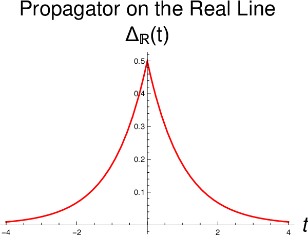
It exponentially decays with with the characteristic time (or life-time)
| (38) |
Let us remark that, since the time ranges in the entire real line, by going to very large times,
| (39) |
one can arbitrarily decorrelate the system, as the exponential can become infinitesimal,
| (40) |
We will see that this possibility does not hold anymore when we define the theory on a circle.
2.4 Renormalization
It is not possible to exactly resum the correlators to all orders in , because one does not know exactly, for general , the coefficient of [9]. One has then to resort to perturbation theory in . The most singular diagram is the tadpole one (a one-loop diagram involving a single propagator), which is ultraviolet finite:
| (41) |
That implies that the renormalization of any parameter of the field normalization constant is finite:
| (42) |
With the canonical normalization of the field which we have chosen, .
Note that a power infrared divergence occurs in the above tadpole for , related to the fact that, in the massless limit, the motion of the particle becomes a free one.
2.5 Analytic continuation to Minkowski space
By means of analytic continuation according to eq.(16), the euclidean correlators become, in Minkowski space, the -ordered products of the field operators averaged over the vacuum state:
| (43) |
Because of eq.(16), the Minkowski correlators are boundary values of the Euclidean correlators for complex times.
We can obtain the propagator in Minkowski momentum (energy) space by means of the following complex rotation66 6 Note the change of sign in the rotation angle with respect to the relation between the corresponding times.:
| (44) |
with the Minkowski (physical) energy. It holds:
| (45) |
We can interpret the above formula as a relativistic propagator in which the energy is replaced by the rest particle mass ,
| (46) |
The latter is a static approximation for both the particle and the antiparticle states.
3 Euclidean Anharmonic Oscillator on a Circle
Since we want to define the theory on a finite lattice with periodic boundary conditions, let us first consider the simpler case of a quantum anharmonic oscillator on a circle, i.e. let us compactify the real line to a circle ,
| (47) |
As regards to topology, we are making a one-point compactification, by adding one point at infinity. As physics is concerned, by going from the real line to the circle, we are basically introducing an explicit time scale in the theory, namely the length of the circle . The parameter plays the role of the ”largest possible time”, in the sense that any time living in is subjected to the limitation
| (48) |
That implies, as we are going to explicitly show, that the exponential decay of the propagator
| (49) |
cannot be observed for any time , namely up to infinitesimal values, unlike the case on the real line. The inverse of the circle length,
| (50) |
is to be considered as an infrared cutoff to the energies :
| (51) |
In this case, unlike the theory on where both time and energy are continuous variables, time is still continuous, while energy is discrete because of the finite size of the circle. The circle is defined, as usual, as a closed segment with its end-points identified
| (52) |
with fixed
| (53) |
is therefore our euclidean time domain. Note that the condition above (endpoint identification) looses its meaning in the limit of an infinite ,
| (54) |
This observation will become relevant when we consider infinite lattices. As well known in mathematics77 7 That is the dual characterization or functional characterization of the circle. , we can forget end-point identification, i.e. take
| (55) |
but restrict to functions coinciding on the end-points
| (56) |
The correlation functions to exactly compute read:
| (57) |
where we have dropped the ”” subscript . The euclidean action has the expression
| (58) |
and the measure reads
| (59) |
3.1 Symmetries
The theory has a global symmetry, related to continuous angle rotations (the subgroup) and discrete reflections of about any diameter88 8 It is a ”compact remnant” of the symmetry of the theory in (see previous section).. If we represent the circle in the plane as
| (60) |
then the action of the group reads
| (61) |
while the reflection for example about the axis is given by
| (62) |
3.2 Free Propagator
The free propagator in momentum (energy) space is obtained from the propagator on the real line by replacing the continuous energies with the allowed discrete energies :
| (63) |
where
| (64) |
Note that the discrete energies are evenly spaced:
| (65) |
The propagator in configuration (time) space is given by the following Fourier series (see fig.2):
| (66) | |||||
Note that it is a periodic function of the time with period ,
| (67) |
as it should.

Let us make a few observations:
- 1.
Since the coefficients of the Fourier series above behave asymptotically as
(68) the function has a discontinuous first derivative at , as can also be seen directly by differentiating with respect to time the first and the last member in eq.(66);
- 2.
In the formal limit , the energy spacing and one recovers the euclidean propagator on the real line:
(69) where
(70) In practice, the propagator on is close to the one on if the sum over the discrete energies , , is a good approximation of the integral over the continuous energies . For that to be true, the denominator on the last member of eq.(66) must not vary much when
(71) This occurs if
(72) Furthermore, also the oscillating exponential at the numerator on the last member of eq.(66) must vary little under the variation (71). That implies its argument must be much less than one, i.e. that it must hold
(73) - 3.
The propagator on roughly decays exponentially with the lifetime for half of the circle length (see fig.2):
(74) The maximal decorrelation, i.e. the smallest possible value of the exponential, is therefore
(75) By requiring to be close to the theory on , we therefore obtain again the relation
(76) If the condition above is not satisfied, finite volume effects are substantial and the theory on the circle has no resemblance to the one in the continuum.
4 Anharmonic Oscillator on an Infinite Lattice
Compared to the theory on the real line, the theory on a lattice of infinite spatial extent contains an additional scale, namely the lattice spacing . Unlike the length ”” of the circle of the previous section, the lattice spacing ”” has to be considered as the ”shortest possible time” in the theory,
| (77) |
Its inverse
| (78) |
plays the role of an ultraviolet cutoff on the energies :
| (79) |
Since the propagator decays by the factor
| (80) |
when we move away from the origin by one lattice spacing, i.e. by the smallest possible distance, in order to be close to the exponential decay on the real line, , , the above factor has to be close to one, so it must be
| (81) |
The doubly-infinite lattice immersed in is written
| (82) |
The theory on the lattice has ”specular” properties with respect to the theory on the circle : time is discrete, while energy is continuous, because the lattice has infinite spatial extent, so there is no infrared cutoff.
4.1 Symmetries
The theory on the lattice has a discrete symmetry group generated by the translation of the time by one lattice spacing,
| (83) |
and the reflection about the point ,
| (84) |
is the crystallographic group of an infinite one-dimensional lattice with a single lattice spacing .

4.2 Free Propagator
The free propagator on the doubly-infinite lattice reads:
| (85) |
Since the r.h.s. of the above equation is a periodic function of the energy with period , the latter is typically restricted to the first Brillouin zone,
| (86) |
In the continuous limit, i.e. in the limit of zero lattice spacing, , one recovers the euclidean propagator on the real line ,
| (87) |
with the energy now ranging in the entire real line,
| (88) |
In configuration (time) space, the propagator reads
| (89) |
where we have defined the effective mass and the effective pole residue:
| (90) |
with
| (91) |
The following remarks are in order.
- 1.
On the lattice , the only ”allowed” times are integer multiples of the lattice spacing,
(92) so that the argument of the exponent on the last member of eq.(89) contains the modulus of the discrete times,
(93) - 2.
The effective mass and the effective pole-residue of the propagator on , unlike the corresponding quantities and in the continuum, do depend on the lattice spacing and have corrections.
(94) As already discussed, the theory has indeed an ultraviolet cutoff provided by (or ), the inverse of the lattice spacing, but no infrared cutoff, because the lattice has an infinite spatial extent. Note that the above corrections are very small.
5 Anharmonic Oscillator on a Circular Lattice
To define an anharmonic oscillator on a finite lattice of size immersed in the circle ,
| (95) |
we discretize the euclidean time , with and the lattice spacing, and define the scalar field at each lattice point as
| (96) |
We will call the lattice a ”circular lattice” when boundary conditions become relevant. The time derivative of the field is discretized as a nearest neighborhood interaction,
| (97) |
By omitting a trivial normalization, the correlators to compute read
| (98) |
where we have introduced the following compact notation:
- 1.
The string of fields at the lattice points,
(99) - 2.
The multi-index
(100) with components, since we are dealing with a bosonic theory, in the range
(101) - 3.
The product of the string of fields with the chosen exponents
(102) - 4.
The integration measure given by an ordinary product of Lebesgue measures on ,
(103) We are indeed dealing with an ordinary multiple integral;
- 5.
The generalized lattice action
(104) where the last coupling involves, because of periodicity, the field
(105) We have introduced a different coupling in each term of to have more freedom in writing evolution equations (see later). In reality, as well known, a given discretization of the time derivative in the continuum action, together with the choice of , unambiguously fixes the couplings and .
Let us end this section with a few remarks.
- 1.
Because of ultraviolet finiteness (finite tadpole), as well as infrared finiteness (), we can assume the bare parameters and entering to be constant in varying the lattice spacing . In other words, the Renormalization Group flow is trivial: we remain in the same physical (low-energy) theory by varying while keeping the bare couplings above fixed;
- 2.
We consider the correlator as a function of the multi-index , i.e. as a discrete function of the exponents of the fields at all lattice points. Unlike classical field theory, where one looks at the lattice fields individually, in the quantum case a ”global” information is needed, involving the simultaneous knowledge of the exponents of the fields at all points. The quantum case is therefore radically more ”correlated” than the classical one, already at the level of formulation.
- 3.
By looking at the expression of one finds that, since the indices can be varied independently from each other at each lattice point, from zero to infinity, we have to compute
(106) independent correlation functions, where is the set of the integers, zero included,
(107) The number of kinematically-independent correlators to compute on a finite lattice of whatever size , is therefore countable
(108) - 4.
As already discussed, to solve a quantum field theory means to know all the correlators ’s, which are average values of monomials in the fields ,
(109) Now, a polynomial in the ’s is a finite linear combination of the monomials above,
(110) where are arbitrary coefficients. Therefore, we may also say that to solve a quantum field theory means to know the expectation values of any polynomial in the ’s,
(111) It is clear that this second formulation of the theory is completely equivalent to the first one.
5.1 Free Propagator
In this section, we derive the free propagator of the theory on the circular lattice . Compared to the theory on the real line, the theory on contains two additional scales, namely the lattice spacing and the length of the embedding circle . These two scales are related to each other by the size of the lattice, i.e. by the number of its points, by the relation
| (112) |
Combining the results of the previous two sections, we derive that the times of the theory on are subjected to the double limitation
| (113) |
If we consider instead the energies , the limitations are ”reversed” and read
| (114) |
In order to have a match of the range of the discrete energies with the range of the continuum energies in the infinite lattice, which we have taken in the first Brillouin zone (86), let us write the points of in a symmetric way, as
| (115) |
where is the integer part of , defined in such a way that the remainder is always positive (e.g. ). The propagator in the energy space is given by
| (116) |
with the integer in the range
| (117) |
In the last member of the above equation, we have simply replaced, in the propagator on the infinite lattice , the allowed, discrete energies in place of the continuous energies ,
| (118) |
The propagator on the circular lattice is obtained via the Discrete Fourier Transform (DFT) of the previous one (see figs.4 and 5):
| (119) | |||||

Let us now discuss the relation of the above propagator with the propagators derived in the previous sections.
- 1.
Continuum limit, i.e. limit of zero lattice spacing, at finite volume, i.e. at finite and fixed ,
(120) In this case, the lattice size diverges, as
(121) The energy spacing does not go to zero, but it is constant in the above limit. The propagator on in the energy space has the limit
(122) with
(123) constant, with the integer now taking any integer value
(124) The exponent is naturally written as
(125) where . Since const., the propagator , on the second member of eq.(119), tends to the propagator on the circle (see fig.4):
(126) As already discussed, the propagator on the last member of the above equation tends to the propagator in the real line for ;
- 2.
Limit of infinite volume, i.e. of infinite time , at fixed lattice spacing ,
(127) The lattice size diverges in this limits as,
(128) Since
(129) we recover the propagator on the infinite lattice (see fig.5):
(130) In turn, the above propagator tends, in the limit of vanishing lattice spacing, as we have seen above, to the propagator on the real line:
(131)

The pattern of the limits considered above can be summarized by the following diagram:
| (132) |
Let us end this section with a few comments.
- 1.
All dimensionfull parameters have disappeared from the propagator in eq.(119), as is adimensional and the length of the circle does not explicitly appear;
- 2.
As already discussed, since the circular lattice is finite, the theory has both an infrared cutoff and an ultraviolet cutoff on the lengths. In order to make finite-volume effects small, one has to take
(133) while, in order to render finite lattice-spacing effects small, one has to take
(134) At a given lattice size , one has to compromise between the two requests, a possibility being given by the ”symmetric choice”
(135) giving
(136) - 3.
According to convenience, we have indexed the lattice points in different ways,
(137) or
(138) Since the circular lattice is clearly invariant under rotations of , we can add to any index an integer multiple of ,
(139) without changing the lattice point. That is equivalent to say that we can identify the above integers
(140) It is therefore natural to think to the circular-lattice indices as elements of the quotient ring
(141) i.e. to take
(142)
5.2 Symmetries
In this section we consider the classical and quantum symmetries of the anharmonic oscillator defined on the circular lattice of size . In general, by regularizing the theory on a lattice, the symmetries of the original continuum theory are, roughly speaking, drastically reduced. One goes from continuous groups, having the cardinality of the continuum, such as the orthogonal group , to finite groups.
5.2.1 Classical Case
Symmetries of the classical field theory are given, as well known, by the invariance group of the action. In the general case, the lattice action,
| (143) |
has not any linear symmetry. Relevant symmetries emerge in the following two particular cases:
- 1.
The coefficients of the terms involving odd powers of the fields vanish:
(144) In this case, the action is even under change of sign of all the fields,
(145) The symmetry group is then the group with two elements
(146) - 2.
The coefficients do not depend on the index , i.e. on the lattice point,
(147) so that the action reads:
(148) For , all the above sums are invariant under the symmetric group acting on the set of all the lattice points . For , the third sum on the r.h.s. of the above equation, having as coefficient, is invariant under the dihedral group , while the other sums are still invariant under . The group , defined for any , is the group of the symmetries of a regular polygon with sides, often called -gone for brevity [10] (see fig. 6 for the case , an equilater triangle, and fig. 7 for , a square).

Figure 6: Equilateral triangle (in black), i.e. regular polygon with vertices (or sides), together with its three symmetry axes (in red). The latter pass through the center of the triangle and anyone of its vertices. An equilater triangle is invariant under rotations about of integer multiples of the angle . Presented in terms of generators and relations, the dihedral group reads:
(149) 
Figure 7: Square (in black), i.e. regular polygon with vertices (or sides), together with its four symmetry axes. Two of them (in blue) coincide with the diagonals, i.e. pass through opposite vertices, while the other two (in red) pass through the midpoints of opposite sides. The square is invariant under rotations about its center of integer multiples of a right angle (). The subgroups of can be obtained as follows.
- (a)
By dropping the generator ”” from the above formula, we obtain the subgroup , the cyclic group of order ,
(150) A regular -gone can be inscribed into a unit circle centered in zero in the complex plane :
(151) By putting one vertex on the positive axis, let’s call it , the vertices of form the set
(152) where we have identified with its vertices. The group can be written as
(153) It holds
(154) The action of the cyclic group on consists in rotating it rigidly by integer multiples of the angle . Such an action is induced on the set of the vertices of :
(155) It is intended that indices are defined modulo ;
- (b)
By dropping instead the generator ””, we obtain the order-two subgroup
(156) which represents a reflection of the -gone about one of its symmetry axes;
- (c)
Given the reflection above ””, other reflections are obtained as
(157) The elements on the r.h.s. of the above relation indeed have order two:
(158) Geometrically, for odd, the reflections are about lines passing through the center of the polygon and one of its vertices (see fig.6). For even, there are reflections with respect to axes passing through opposite vertices and reflections with respect to axes passing through the midpoints of opposite sides (see fig.7).
From the above calculations, it follows that is a group of order , i.e. it contains elements. For any , it clearly holds
(159) Since for ,
(160) it follows that in this case these groups coincide:
(161) Since, for ,
(162) it follows instead the dihedral group is a proper subgroup of the symmetric group,
(163) Roughly speaking, we may say that the dihedral group is the ”discrete remnant” of the orthogonal symmetry group of the continuous theory on . To be more specific, we may say that:
- (a)
The cyclic group is the ”discrete remnant” of the special orthogonal group because, while in the continuous case we can rotate a circle around its center by any real angle, in the discrete case we can rotate an -gone only by integer multiples of ;
- (b)
The reflections in are the discrete remnant of the reflections about any diameter of .
Because of eq.(159), we conclude that the action in eq.(148) has for any the symmetry group
(164) Explicitly,
(165) where by we denote the action of the group element on the lattice point.
Random Field
We may ask ourself what happens to the action in eq.(148) if we set to zero all the coupling between different fields, i.e. if we take
(166) In this case there is no more correlation between fields at different points and the theory describes a random field. For , the term under consideration explicitly reads
(167) and is symmetric under exchange of the indices and , like all the other terms in ; the symmetry group is . For , the term proportional to is
(168) and has again the same symmetry of the other terms in . For , one has a polynomial in the ’s given by
(169) which is invariant only under and not under . That occurs because is not a symmetric polynomial, as it does not contains the monomials
(170) A similar phenomenon to the latter one also holds for any . The conclusion is that, if we take
(171) then the action becomes invariant under the full symmetric group,
(172) which is a much larger group than the dihedral one for .
- (a)
- 3.
Both symmetries above. The action in this case reads
(173) The theory then has both a and a symmetry. Since acts on the values of all the fields , , without touching the indices, while acts on the indices of the fields, without touching their values, these two groups commute with each other and the resulting symmetry is given by their direct product:
(174)
5.2.2 Quantum Case
In looking at the symmetries at the quantum level, we have also to look at the integration measure
| (175) |
The measure above is invariant under:
- 1.
Change of sign of all the fields,
(176) because the jacobian of the transformation has modulus equal to one;
- 2.
Action under the symmetric group , because
(177) The differentials of the fields indeed commute with each other.
As a consequence, the classical symmetries go over into the corresponding quantum symmetries or, in other words, there is no anomaly. Let us then reconsider the classical symmetries of the previous section, which now take the form of Ward identities relating different correlators among each other.
- 1.
Symmetry. It implies that all the correlators with an odd sum of all the exponents identically vanish:
(178) - 2.
Symmetry. It implies on correlation functions that:
(179) For a given , let us now consider lattice indices (which exist and are uniquely defined) such that:
(180) so that
(181) It follows that
(182) Let us define
(183) Since takes values in the whole group as we vary in all , the above equation is rewritten as
(184) It expresses the action of the symmetry on the correlators.
Let us define the sum of all the exponents (indices) of a given correlator
(185) Since
(186) the symmetry group relates correlators with the same weight. In other words, is an invariant, as it commutes with the action of . That implies, for example, that a 2-point correlator with (i.e. a propagator) will never mix with a 4-point function of the elementary fields, having .
As already discussed, the action of , the cyclic group of order , on a lattice point reads
(187) Invariance under implies
(188) where is any integer. As usual, it is intended that indices in the last equation are defined modulo .
In general, we will call equations of the above form Lattice Symmetry Equations (LSE). We will use the above symmetries in the next sections. The idea is that, as far as the counting of independent correlators is concerned, we go from individual correlators to orbits of correlators.
6 Continuum Limit of the Theory on
Suppose we want to describe hadron dynamics by means of an euclidean space-time lattice. Since the typical dimension of a hadron, such as a proton or a meson, is of the order of one Fermi,
| (189) |
we expect that a box of a linear dimension of, let’s say, ten Fermi’s should be reasonably good,
| (190) |
Let’s then imagine to fix to the above value. The lattice spacing is given by
| (191) |
where is the lattice size. The continuum limit is defined as the limit of vanishing lattice spacing 99 9 If the theory contains for example a particle with mass , as in our case, that physically means to send to zero the adimensional quantity , (192) If only massless particles are involved, then one may require for example (193) where is the lowest non-zero energy.,
| (194) |
According to eq.(191), it implies that the lattice size diverges:
| (195) |
Actually, while increasing , one can also increase in order to render finite-volume effects vanishing small, so long as the lattice spacing still goes to zero. Let us make a few observations.
- 1.
Taking the continuum limit while keeping the lattice size fixed implies
(196) i.e. one goes to the continuum, but in an infinitesimal box, which is not what physics usually requires;
- 2.
The limit of infinite lattice size does not necessarily implies the continuum limit. Indeed, one can take the limit while keeping constant, implying that one is taking the dimension of the box growing exactly as .
To solve the theory means to obtain analytical expression of the correlators
| (197) |
where the lattice action is given by the following series:
| (198) |
We have used an explicit notation in order to stress the difference with respect to the finite case. While for any finite lattice size, , there is only one possibility in defining what we mean by analytic solution, in the continuum limit there are instead two different possibilities, which we call the strong limit and the weak limit.
- 1.
Strong Limit. That is the first possibility that comes to mind. One considers all the possible values of the multi-index
(199) which can be thought of as a map from the ring of the integers to the natural numbers:
(200) where the set of the natural numbers is defined as including the zero,
(201) According to this definition of solution of the theory, the knowledge of correlators such as for example the one with for any ,
(202) is then required. The cardinality of the correlators to evaluate is then
(203) which is the cardinality of the continuum. Along this route, we find an intractable theory. However, at this point, physics comes to our help: we know that only correlators with a finite number of points --- though arbitrarily large --- are needed:1010 10 For example, at the Large Hadron Collider (LHC), presently operating at the European Center for Nuclear Physics (CERN) at a Center-of-Mass energy of 13 , processes with up to partons in the final state are studied.
(204) Indeed, if we consider scattering processes of particles with a mass at any given energy , then the number of particles in the initial state, , and in the final state, , is subjected to the upper kinematic bound
(205) The above bound is empty in the case massless particles (), such as photons or gluons, are involved in the process. In such cases, as well known, if infrared divergences are present, one is forced to consider correlators with an arbitrarily large number of particles, yet still finite. To summarize, as far as physics is concerned, correlators with an infinite number of points are not relevant. This observation offers us the possibility to define a simpler continuum limit.
- 2.
Weak Limit. A much simpler theory, with the same physical content as the above one, is obtained if we require the (infinite) sum of all the occupation numbers to be finite:
(206) We then require all the infinite occupation numbers , , to be zero, except for a finite number of them.1111 11 It’s like to have an infinite number of distinguishable boxes, but only a finite number of balls to put inside them. Only finitely many boxes are not empty. In other words, the ’s become definitively zero going in the positive direction, , as well as going in the negative direction, . That is to say that we restrict to maps
(207) which are definitively zero. Let us denote the set of such maps with the symbol
(208) Correlators such as the one considered in the previous point, with for any ,
(209) are then excluded from the definition of solution of the theory.
As already discussed, for finite lattice sizes, , the theory can also be formulated in terms of average values of polynomials in the ’s, :
(210) In the continuum case, we may also say that solving the theory means to know the average value of an arbitrary polynomial in the infinitely many variables ,
(211) where the dots at the beginning and at the end of the string denote that there is neither a first variable nor a last variable.
Going back to correlators, we can assign to each two characteristic numbers:
- (a)
The sum of all the indices,
(212) The vacuum correlator, having all its indices equal to zero,
(213) for example, has
(214) Correlators with one non-zero index at any point ,
(215) have
(216) and so on. We will see that the above integer number will play an important role when we will discuss the dynamics in the continuum limit;
- (b)
The number specifying how many indices are not zero, but strictly positive. Given
(217) let us define
(218) For any correlator , it clearly holds
(219) Correlators with one non-zero index at any point ,
(220) for example, have . Note that, since the non-zero index can be put at any place, it follows that
(221) since the direct product of a finite family of countable sets is countable. is the set of strictly positive integers,
(222) Correlators with exactly two strictly-positive indices
(223) have . For the first index we can take any position , while for the second index we can take any position with . The cardinality of the correlators with is therefore given by
(224) Since each correlator has a well-defined value of , the set of all ’s can be written in the form:
(225) where the union is disjoint, i.e. it involves pair-wise disjoint sets.
Since the union of a countable family of countable sets is countable, we conclude that the set of all correlators is countable in the weak limit:
(226) That has to be compared with the strong-limit case, in which the correlators have instead the cardinality of the continuum. Therefore, by requiring the indices or to be finite for any , we reduce the cardinality of the correlator set from to .
- (a)
The difference between the strong and the weak limits can be easily understood by means of the following simple example. The weak limit is the analog of the vector space of all the polynomials in one indeterminate , let’s say on the real field,
| (227) |
The latter is an infinite-dimensional space, having as algebraic (or Hamel) basis, for example, the countable set of all the monomials
| (228) |
The vector spaces of all the polynomials with degree up to ,
| (229) |
form a strictly-increasing sequence (filtration) of finite-dimensional vector spaces
| (230) |
whose union is the space under consideration:
| (231) |
The strong limit is the analog of the vector space of all the formal power series:
| (232) |
The latter is a much bigger vector space,
| (233) |
which cannot be invaded by sequences of finite-dimensional spaces, with an uncountable algebraic basis.
6.1 Symmetries
We expect the lattice theory to acquire, in the continuum limit , symmetries described by finite or infinite discrete groups.
- 1.
Symmetry. The invariance of the theory under change of sign of the fields on a finite lattice of size ,
(234) simply becomes, in the limit :
(235) - 2.
Symmetry. The ”limit” of the dihedral group can be simply defined by removing the condition (which becomes meaningless) from the definition:
(236) An infinite abelian subgroup of is the free group generated by the element :
(237) As well known, the above group is isomorphic to the additive group of the ring of the integers,
(238) By acting on the reflection as
(239) one generates a countable number of reflections. It is straightforward to check that the symmetric lattice action
(240) is invariant under , so let us just sketch the proof. The action above is invariant under any shift of the index
(241) i.e. it is invariant under . If we identify the symmetry ”” with the reflection about the lattice point ,
(242) then is invariant under such transformation. Since we have already proved the invariance of the action under the group , it follows that is also invariant under the action of , , and then under the complete dihedral group .
If we set to zero the coupling in the action in eq.(240), then the theory becomes invariant under the symmetric group , the symmetric group acting on the infinite set of the natural numbers,
(243)
7 Dyson-Schwinger Equations on the Lattice
Linear relations between the correlators ’s are obtained by means of the Lattice Dyson-Schwinger (LDS) equations:
| (244) |
By explicitating the derivatives, one obtains
| (245) |
with or, more explicitly,
| (246) |
In a more compact notation,
| (247) |
Going back to the index notation, one obtains the set of equations:
| (248) | |||||
with
| (249) |
The term on the first line above vanishes for . The shifted indices have been put inside curly brackets for clarity purposes. Let’s make a few comments.
- 1.
If we had discretized the time derivative of the field by using also next-to-nearest differences, also a term of the form
(250) would have appeared in the LDS equation above;
- 2.
In a theory with a cubic interaction, such as for example a theory,1212 12 It is well known that the theory does not exist because the cubic potential is unbounded from below for any real , so the functional integral is divergent. By giving up unitarity, we can formally overcome this difficulty by taking purely imaginary. the last term of the LDS equation would have the index replaced by . If the theory under study involves different interactions, the sum of the corresponding contributions does appear.
If we define the observables of the quantum field theory by means of average values of polynomials in the ’s,
| (251) |
with
| (252) |
then the lattice Dyson-Schwinger equations are written as
| (253) |
In a more compact notation,
| (254) |
where is any polynomial in the ’s.
7.1 Examples
To get some intuition concerning the LDS systems, let us see a few examples on small lattices:
- 1.
For there is the LDS equation
(255) Being there only one field, one can only study self-correlations of the single field with itself. In the gaussian case,
(256) the LDS equation becomes a simple two-step, two-term equation
(257) - 2.
For one has the two LDS equations:
(258) This is, in some sense, the lowest-order non-trivial case, involving correlations at two different points. The gaussian theory corresponds to
(259)
8 Solution of Lattice Dyson-Schwinger (LDS) Equations
In general, in order to solve a model, one has to combine all the information available. In our case, a theory on a lattice, one has to combine together the Lattice Dyson-Schwinger Equations (LDS) with the Lattice Symmetry Equations (LSE). However, in order to understand the general ”philosophy” of our study, let’s neglect the symmetry equations to begin with — they will be included later.
We have one LDS equation for each lattice point and for each possible choice of the index . So, by substituting all possible numerical values for all the indices, we get a huge linear homogeneous system on all the correlators ’s. In physical language, the quantum equations of motion produce linear relations between the kinematically independent correlators. There is an infinite number of unknown correlators ’s and an infinite number of equations, so the solution of the system is, a priori, not trivial at all. Since the system is homogeneous in the correlators, one has to arbitrarily decide which correlators are to be considered as known — i.e. to be put on the right hand sides of the final solutions — and which are to be considered as unknown — and then kept on the left hand sides. It is somewhat natural to solve the above system by expressing correlators with large values of the indices in terms of correlators with smaller values of the indices. This idea can be formalized by defining a recursive weight, defined individually for each correlator, which involves, for example, the sum of all the indices in ,
| (260) |
The correlator with the lowest possible recursive weight, for example, is the vacuum amplitude , having weight zero:
| (261) |
The propagators,
| (262) |
have and so on. The terms on the symbolic LDS eq.(248), in the same order in which they are written, have the following weights:
| (263) |
where is the symbolic sum of all the ’s:
| (264) |
Note that all weights above differ from each other by an even number (zero,two and four), because the action is even in .1313 13 If we were to add to terms linear or cubic in the ’s, then odd differences between the ’s would appear. The parity of would not be respected in correlator decomposition.
The term with the highest weight is then the last one in eq.(248), the quartic one, which represents the interaction in our model. In the interacting case , eq.(248) is a 4-step recurrence equation. As expected from experience, there are three regimes in which equation (248) drastically differ, the first two being infinitely simpler than the third one.
- 1.
Random Field,
(265) in which the LDS equations loose the couplings between different lattice points. The fields at various lattice points fluctuate independently on each other, in non-gaussian way for . As a consequence, there is not any wave propagation and correlations at different points;
- 2.
Gaussian or Free Theory,
(266) in which the action become quadratic in the fields and the LDS equations reduce to 2-step recurrence equations — note the discontinuity. We recover in this case the standard gaussian theory (Wick theorem);
- 3.
Fully-interacting Theory,
(267) in which both propagating and anharmonic effects are fully retained. This is our main concern.
8.1 Random Field
The LDS equations reduce in this case to the following ones.
| (268) | |||||
In the non-gaussian (anharmonic) case
| (269) |
the solution reads:
| (270) |
The shifted index (we have not changed the symbol) has the restriction , while the other indices have the usual range:
| (271) |
The first term on the r.h.s. vanishes for . It is a lucky circumstance that there is only one correlator with maximal weight , so it has not been necessary to take linear combinations of different LDS equations.
8.1.1 Random Gaussian Field
In the Gaussian case the LDS equations reduce to two-terms equations
| (272) | |||||
The solutions read:
| (273) |
For the r.h.s. of the above equation vanishes.
8.2 Gaussian Theory
In this case, the -th (symbolic) LDS equation contains three correlators,
| (274) |
having the same (maximal) weight,
| (275) |
and one correlator,
| (276) |
with a weight smaller by two units,
| (277) |
The LDS equations are then naturally written in this case as
| (278) |
with . Note that we have slightly simplified the notation:
| (279) |
By varying the index equation in the entire range , we obtain linearly independent equations, which can be solved for the correlators, each one having one index increased by one unit, namely:
| (280) |
The known terms are linear combinations of all the correlators with one index lowered by one unit, namely:
| (281) |
The solutions are then of the form
| (282) |
The coefficients can be explicitly calculated by inverting the tri-diagonal matrix
| (283) |
We are indeed solving the Poisson equation with a mass term added, on a one-dimensional lattice immersed in a circle, with known terms given by lower-weight correlators.
For computer applications, it is natural to have the l.h.s. of the equations (282) to contain unshifted indices. By means of the shift
| (284) |
the solution (282) is rewritten as
| (285) | |||||
where we now have the restriction on the indices
| (286) |
By using the above set of equations, one is able to express an arbitrary correlator , with , as a linear combination, with known coefficients, of correlators with . By means of an iteration, one can express in terms of correlators with and so on. By iterating this procedure up to the boundary values for the indices, one can then reduce any correlator to a combination of correlators with weight
| (287) |
namely the vacuum correlator ()
| (288) |
and the tadpoles ()
| (289) |
In a symmetrical theory for , such as our reference theory, odd correlators vanish, so that all correlators can be expressed as a multiple of the vacuum correlator,
| (290) |
where is a known function depending, in addition to the indices, also on the couplings and of the model.
8.2.1 Examples
Let us consider in this section a few examples of reduction of Gaussian correlators.
- 1.
Propagator. By that we mean the correlators1414 14 We assume that and may coincide (), giving rise in this case to the correlator with , . with
(291) which can be expressed in terms of the vacuum correlator only,
(292) in just one step;
- 2.
Explicit Solution at . Let us discuss the explicit solutions of LDS equations in the free (or gaussian) case for . By solving the two symbolic equations (258) with respect to the two higher-weight corrrelators, we obtain, after trivial shifts of the indices:
(293) Let us make a few comments.
- (a)
The singularity for
(294) originates from a massless zero mode;
- (b)
By replacing the numerical values
(295) one obtains the reduction of the propagator to the vacuum amplitude
(296) - (c)
For , the couplings between different indices disappear.
- (a)
8.3 Fully-interacting Case
In the fully-interacting case,
| (297) |
we solve eq.(248), as explained, in terms of the last amplitude on the rhs of (248). It is then natural to make the shift on the -th index only
| (298) |
The symbolic solution of the LDS equation reads:
| (299) | |||
The shifted index (we have not changed the symbol) has the restriction , while the other indices have the usual range:
| (300) |
If more than one correlator with maximal weight had occurred in the LDS equations, it would have been necessary to take linear combinations of them. Let us comment upon the various terms on the r.h.s. of the reduction equation.
- I term:
It reduces the current occupation number by four units;
(301) Since it does not touch any index with , it is ”diagonal” in index space. It is the only term with a coefficient depending on and it vanishes for ;
- II term:
It reduces the current occupation number by two units:
(302) It is also a diagonal term, in the sense specified at the previous point;
- III term:
It decreases the current index by three units and at the same time it increases by one unit the index to the left of ,
(303) It is non diagonal in index space and will be called a Left Mover (LM), as it transfers part of the value of to ;
- IV term:
It is the last one and it acts analogously to the previous one,
(304) It will be called a Right Mover (RM).
The fundamental point is that, by repeatedly using the above equation, for different indices and for different values of the occupation numbers , one can reduce an arbitrary correlator to a (finite) linear combination, with known coefficients, of correlators having all indices less than or equal to two:
| (305) |
where we have defined the multi-index
| (306) |
We call the correlators which appear on the right hand sides of the complete reductions primitive correlators and we have denoted them by ,
| (307) |
The irreducible correlator with the highest weight has all its indices equal to two and
| (308) |
where is the lattice size. Let us make a few remarks:
- 1.
Many different reduction paths are possible in index () space. Since the final result is well defined, it follows by consistency that they are all equivalent;
- 2.
Each time the equation above is used an over-all factor
(309) enters the decomposition. Large (but finite) inverse powers of the couplings then enter the decomposition of any correlator;
- 3.
In general, correlators with many large indices, i.e. with a high weight , involve a massive reduction process before primitive correlators are finally reached. Let us remark however that the number of reduction steps is finite in any case, because at each step we generate correlators with weight reduced at least by two units. However, it may happen that also correlators with relatively small weights may undergo a long reduction process, with a large number of primitive correlators appearing in the final formula. We will see explicit examples of these phenomena in a moment.
8.3.1 Examples
In this section we present some simple explicit examples of solutions of LDS equations.
- 1.
Long Reduction Chain. A long reduction chain is obtained by considering for example the correlator
(310) having one index equal to zero, the adjacent one to the right equal to three, with all the other indices equal to two. Since only the first index is greater than two,
(311) the first reduction step necessarily involves eq.(299) for . Let analyze in turn the generated terms on the r.h.s.:
- I term:
It vanishes, as already noted;
- II term:
It produces a primitive corrrelator,
(312) because it just shifts
(313) by keeping the remaining indices unchanged;
- III term,
the : it also produces the primitive correlator
(314) It reduces to zero the index equal to three,
(315) and at the same time increases by one unit the index to the left
(316) Index increase is ”potentially dangerous”, in the sense that it produces in general reducible correlators, but this is not the case because we have chosen an initial small value of .
- IV term,
the RM: it produces a reducible correlator,
(317) That is because, as in the previous case, the current index has been reduced below the critical value ,
(318) but the index to the right, , was initially set to two , so by increasing it by one unit we go above the critical value:
(319)

Figure 8: Effects of the operators for , in order, on the string of indices . The peak corresponding to moves to the right by leaving behind him trailing zeros. In summary, with the first reduction step, we have produced three (non zero) correlators: two primitive correlators and one reducible correlator. The second reduction step then only involves
(320) Since , one needs the LDS equation with . The analysis is similar to the previous one: only the RM produces a reducible correlator, because it makes the transition
(321) At this point, the mechanism should be clear: when an index equal to two is to the right of an index equal to three, then the RM increases it, producing a reducible correlator. By considering the RM only (see fig.8),
(322) Since to the right of the index equal to three there are only indices equal to two, by iterating, one finds that the index “three” propagates through all the lattice, by leaving zeroes behind him. A sort of ”wave peak” propagates along the whole lattice, resembling those games with sequences of Lego elements falling progressively on each other. This example can be generalized, in the sense that basically nothing changes, by taking
(323) It is remarkable that we are not solving some wave equation, but we are building up the r.h.s. of an equation. The complexity inherent in solving a wave equation is transferred, in some sense, to the equation itself. The variables seem to represent a current coupling to a pair of neighboring fields and — a generalization of the well-known Schwinger current coupled to the local field .
- I term:
- 2.
Propagation on both directions of the lattice. Let us consider a correlator with all its indices equal to two, with the exception of one index equal to three, such as
(324) In this case, more symmetrical than the previous one, both LM and RM generate recursions chains along all the lattice;
- 3.
Cutting a Long Reduction Chain. The reduction of example 1 propagates an index equal to three on the whole lattice, because in any reduction step, an index equal to three only finds indices equal to two to its right. To ”break” such a propagation, one just needs to insert an index equal to zero or equal to one ”along the way” of the path of the index equal to three,
(325) where is some selected lattice point. The above correlator has a reduction chain to primitive correlators which stops at because
(326)
8.4 Generalizations
By a similar analysis, in a model with a cubic interaction, such as for example a theory, one would be able to shift any index to
| (327) |
The number of primitive correlators on a lattice of size would then be
| (328) |
again with the power of the continuum in the strong limit . With a general interaction Lagrangian with maximal anharmonicity , by solving with respect to the highest weight term, having the shifted index
| (329) |
one would be able to shift inside the range
| (330) |
9 Operator Algebra of LDS Equations
In operator language, the solution of the symbolic LDS equation can be written as:
| (331) |
where the operator is defined as the following sum of linear operators:
| (332) |
having the expressions
| (333) | |||||
| (334) | |||||
| (335) | |||||
| (336) |
The operators on the r.h.s. of the above equations, in turn, are defined as follows:
- •
is the state occupation-number operator i.e., when applied to a correlator , it returns the occupation number of the state, namely ,
(337) In more compact notation, by writing only the relevant indices,
(338) - •
is the raising/lowering operator of the occupation number for the state, i.e. the operator raises/lowers the index by one unit:
(339) with . More briefly,
(340) Even more briefly,
(341) Powers are defined in straightforward way:
(342) so that
(343) and so on (, , etc.). The zero power is the identity operator,
(344) with
(345)
The main properties of these operators are given in the following.
- •
and commute for any lattice indices and and any powers and :
(346) - •
and , , do not commute with each other, as well known from elementary quantum mechanics:
(347) For , for example:
(348) Commutativity holds instead for different indices
(349)
9.1 Examples
Let’s then see a few examples of application of the above rules.
- 1.
It follows from eq.(346) that the operators , and entering commute with each other even for different indices:
(350) - 2.
According to eq.(347), the operator can also be written with the occupation-number operator acting after :
(351) - 3.
The square of the operator reads:
(352) It vanishes for ;
- 4.
The commutation rules of with the other operators entering read:
(353) - 5.
Since commutes with ,
(354) This formula can be used, for instance, to understand the form of the reduction of a correlator having all indices equal to zero, except one index equal to a large value, let’s say :
(355) The indices and increase their value from zero up to , i.e. up to the integer part of one-third of the initial large index value. If or , one has then to apply or respectively, which in turn increase neighboring indices of and up to the integer part of one-third of their values. In total, some sort of diffusive behavior manifests itself, with the initial peak value of spreading out, with ”some loss”, in a neighborhood of the lattice point ;
- 6.
Since also commutes with and , the simple generalization of the above formula holds:
(356) where the dummy indices are non-negative, , and ;
- 7.
The calculation of the general power of the operator is not easy because the operator does not commute with , and . By defining
(357) the most explicit formula we could find is simply
(358) with . One has then to use the commutation rules in eq.(353);
- 8.
As regards the composition of operators entering the ’s for different indices, for , the following formula holds:
(359) - 9.
Concerning the product of RM operators with adjacent indices, the following expression is found:
(360) This formula simply accounts for the form of the long reduction chain considered in an example in a previous section;
- 10.
Since the reduction of any correlator to primitive correlators is well defined, i.e. it does not depend on the reduction path, by consistency it must be true that
(361) The above result can also be checked by explicit calculation;
- 11.
The individual operators entering commute with the operators entering if the indices differ at least by two units, i.e. .
10 Geometry of LDS equations
The rules to solve the LDS equations can be formulated in the following geometric setting, giving rise to a discrete geometry, of high dimension for .
We introduce the index space or -space
| (362) |
The space is an -dimensional lattice space, infinite on one side of each of its dimensions (see fig. 9 for and fig. 10 for ). An arbitrary correlator is represented in this space by a point ,
| (363) |
Since one can make linear combinations of the correlators ’s, has the structure of a vector space.


A norm for a vector can be defined as
| (364) |
As well known, the above norm induces in the following homogeneous and translation-invariant metric:
| (365) |
where
| (366) |
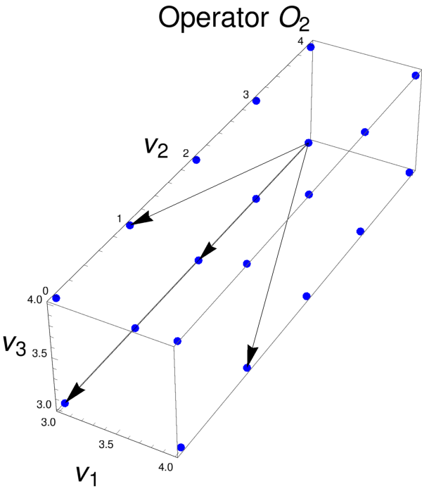
The set of all primitive correlators is represented in the space by a hypercube of edge size equal to two, with one vertex at the origin:
| (367) |
All the vertices of belong to some coordinate hyperplane
| (368) |
with the exception of the highest-weight correlator
| (369) |
We may also write
| (370) |
Note that, for example,
| (371) |
while the ”distance”, as far as the reduction to primitive correlators is concerned, is clearly larger in the second case compared to the first one. To describe the difference between the above cases, it is convenient to introduce a second norm on :
| (372) |
The inequality holds
| (373) |
The induced distance from the one-norm reads
| (374) |
With the new distance,
| (375) |
while
| (376) |
We may also define the distance of a generic correlator , identified by the point , from the hypercube :
| (377) |
Such a distance clearly vanishes if is a primitive correlator.
10.1 Reduction to Primitive Correlators
Let us now discuss the reduction of an arbitrary correlator to primitive correlators. This reduction involves paths along a tree in the space , with the trunk beginning at and with all the branches ending inside . As already observed, there is no a canonically-defined path, but many equivalent paths.
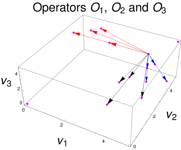
The four operators , , and entering the operator solving the LDS equation can be represented to the following four vectors in the space respectively:
| (378) |
where only the relevant vector components have been written (see figs. 11 and 12). To apply the operator to a correlator is equivalent to adding to each one of the above vectors:
| (379) |
Four points in the space out of one point are then generated. If some of the above points fall within the cube , they are not transformed any more.
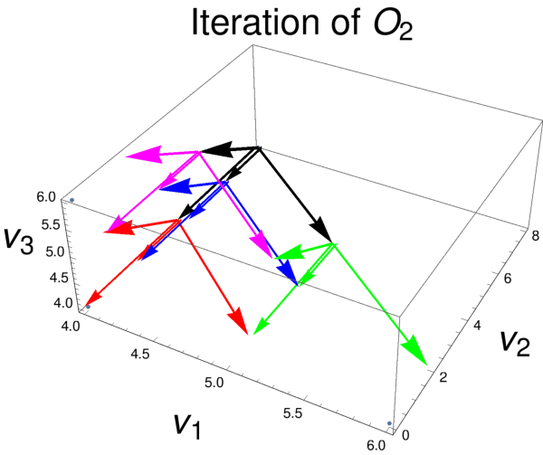
Next, we iterate the above procedure, by applying the operator with the new index , to each one of the four points above (see figs. 13 and 14).
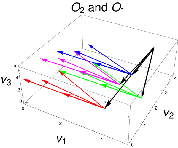
Any index is in principle good, so long as for the current term, because LDS equations with different indices commute with each other and each one of them reduces the weight . In general, each of the four points above generates four terms on his own, so that, after two reduction steps, we have in general points. By iterating the process times, one obtains up to points. The iteration process above can be described as the branching of a quaternary tree. The root of the tree, the trunk, is placed in the initial point . At each step, each branch produces four new secondary branches and so on. The branching terminates when all the current branches fall inside the cube . The branching is in general quite heavy on the computational side, because of the exponential increase described.
The generation of long reduction chains for correlators with an index equal to three adjacent to a long sequence of indices equal to two, such as for example
| (380) |
can be viewed geometrically as follows. The one-distance of the above correlator from the hypercube of the primitive correlators is only one,
| (381) |
With the first reduction, with , we get closer to along the second direction, as
| (382) |
but we become more distant to in the neighboring directions, as
| (383) |
We then have to reduce the distance along the above directions, by applying the LDS equations for and . In general, by getting closer to , by three units, in the direction,
| (384) |
we become more distant, by one unit, in the neighboring directions,
| (385) |
This phenomenon is represented in fig. 15 for . In general, if the lattice size is large, there are many different directions one can take in the space , so that one can move quite a lot in the course of the reduction process of a correlator having even with a small one-distance from , before reaching primitive correlators.

10.2 Evolution Equations for Primitive Correlators
The derivation of a primitive correlator with respect to can also be viewed geometrically in the space . With the derivation, the point in corresponding to is translated by the vector
| (386) |
i.e.
| (387) |
Now, a primitive correlator is represented by a point lying inside . If the shifted point lies again inside , then the derivation has produced another primitive correlator and we have a one-term differential equation. Otherwise, the derivation has produced a reducible correlator. If a primitive correlator lying on the boundary of is derived with respect to , independent correlators with a long reduction chain are in general generated.
11 Inclusion of Lattice Symmetry Equations
Let us now discuss the effects of Lattice Symmetry Equations on the reduction of kinematically-independent correlators to primitive correlators , i.e. to dynamically-independent correlators. Such a reduction has been made in the previous section by disregarding the symmetries of the theory. It is clear that reduce, in general, the number of primitive (i.e. non zero and independent) correlators existing at a given lattice size .
In general, if the theory at lattice size has a symmetry described by a finite group , then the number of primitive correlators satisfies the lower bound
| (388) |
where is the order of , i.e. the number of its elements. The inequality above follows from the fact that any orbit of primitive correlators under contains at most (distinct) elements.
Let us now consider in detail the symmetries of the anharmonic oscillator on a circular lattice considered before.
- 1.
Even Lattice Action,
(389) Since, as already discussed, correlators with odd weight are zero, the number of primitive correlators is roughly reduced by a factor two,
(390) In this simple case, the combination of the LDS equations with the LSE is rather trivial, as they are basically independent. The LDS equations indeed involve corrrelators all having the same parity of the index , i.e. all the correlators entering a given equation all have even or odd ;
- 2.
Lattice Action invariant under the dihedral group ,
(391) This case is more complicated than the previous one, because now combining together the restrictions coming from both the LDS equations and LSE is not trivial.
Since is a finite group with
(392) according to the general inequality (388), it holds
(393) At most, a mild, power-like suppression in the number of primitive correlators is then obtained,
(394) with and .
The basic exponential growth with the lattice size in the number of primitive correlators, which we have found in QFT, can be compared with the situation in classical field theory (which can be considered the limit of QFT for ). Indeed, one can put on the lattice also a classical field theory. If we consider for example a classical scalar field in space-time dimension , discretized on a space lattice of size , the state of the system at a given time is represented by the values of the fields at the lattice points , ,
| (395) |
If we deal for instance with a Cauchy problem, one has typically to integrate evolution equations of second order in of the form:
| (396) |
Each one of the real numbers above, , can be well approximated by, let’ say, a binary expansion with digits with .1515 15 As well known, convergence is exponentially fast in the number of the digits, as the relative error is ; By adding one digit, one doubles the accuracy. Now, if we double the lattice size, i.e. if we go from to , the number of state variables and of evolution equations simply doubles, i.e. there is a linear (power-like) growth with , in contrast to the exponential growth which we have found in the quantum case. The quantum field theory case is therefore intrinsically much more complicated than the classical field theory case.
12 Reduction to Primitive Correlators for
In the weak limit , the index space becomes an infinite-dimensional discrete space,
| (397) |
However, the reduction of an arbitrary correlator
| (398) |
to a linear combination of primitive correlators
| (399) |
is always finite, i.e. it involves a finite number of step in any case. That is because we require the sum of all the indices to be finite,
| (400) |
and, at any reduction step, the above sum is decreased at least by two units. Since, at each reduction step, the number of correlators involved grows at most by a factor four, it follows that the number of primitive correlators appearing in the final decomposition of any is finite. The following remarks are in order.
- 1.
While always finite, an arbitrarily large number of indices in can be different from zero while, at finite lattice size , such a number is obviously limited by ;
- 2.
In the case of the strong continuum limit, since condition (400) is not imposed, the sum of the indices is generally infinite, so that the reduction to primitive correlators involves an infinite number of steps.
12.1 Imposing Lattice Symmetry Equations
By combining the LSE with the LDS equations, two scenarios are in principle possible in the weak limit :
- 1.
Normally-Symmetric Case — or more simply Normal Case. There can be many , but the reduction of the dimensions of at finite lattice sizes , after imposing the , is not so strong to be able to reduce the cardinality of the basis in the limit , which remains the countable one
(401) In this case, the addition of to equations does not play, as far as the reduction to primitive correlators is concerned, any critical role. There is not any ”collapse” of the cardinality of from the countable one to a finite one and the theory is classified as unsolvable;
- 2.
Exceptionally-Symmetric Case — or simply Exceptional Case. There are so many LSE — independent on each other, as well as on the LDS equations — that the cardinality of the primitive correlator basis is diminished from the countable one to a finite one:
(402) That implies that all the primitive correlators of the theory can be expressed in terms of a finite number of them. In other words, after imposing the Ward identities of the theory, only a finite number of independent primitive correlators is found, as in the case of the Gaussian theory. In such an ”infinitely symmetric” case, there is a ”collapse” in the size of the primitive correlators basis and, according to our philosophy, the theory is classified as solvable.
12.1.1 Examples
In this section we consider a few examples of systems with different symmetries.
- 1.
Anharmonic Oscillator on an infinite lattice with symmetry group , the dihedral group of infinite order defined previously. That is the continuum limit of our reference model. The infinitely-many primitive correlators with ,
(403) can be reduced to the two primitive correlators
(404) by means of the shift of the indices , . The symmetry is then very ”efficient” in this case, as it reduces an infinite set of primitive correlators to a finite one. However, the primitive correlators with ,
(405) can only be reduced to primitive correlators of the form
(406) by means of the shift of the indices , . If the indices and are different from each other, one can use the reflection symmetry to render for example , but no further reduction is possible. In the latter case, the symmetry is not so efficient: the number of primitive correlators after the reduction is still infinite. The conclusion is that, in the limit , the number of primitive correlators of the anharmonic oscillator is countably-infinite so the model, according to our definition, is a normally-symmetric one and therefore is unsolvable;
- 2.
Scalar theory for invariant under , the full symmetric group acting on . The action reads:
(407) The latter can also be written as
(408) In a plane, we can have up to three points at the same distance from each other, by putting them at the vertices of an equilater triangle. If we construct a lattice theory on such a triangle, the field at each site interacts in the same way with the fields in the other two lattice points. In the ordinary, 3-dimensional space, we can defined a lattice theory on a regular tetrahedron, and so on. Therefore, the theory above can be naturally constructed in a infinite-dimensional ambient space.
Since, as already discussed, the integration measure
(409) is invariant under , also the quantum theory has the full group as its symmetry group. Any primitive correlator has a string of indices equal to an infinite sequence of zero’s, one’s and two’s. By using the symmetry group , one can reduce any primitive correlator , with , to primitive correlators with the first indices , , , equal to two, the next indices , , , equal to one, with , and all the remaining indices identically zero:
(410) For any given , there are therefore independent primitive correlators. Since the variable can take any integer value,
(411) the theory, despite its large symmetry group , has an infinite set of primitive correlators, so it is classified as unsolvable. Actually, we tried to explicitly solve this model, but we did not succeed, so it seems, at least relative to this example, that our classification scheme is practically relevant;
- 3.
Symmetric Random Field, i.e. the scalar theory for for . As we have seen, this model is invariant under . There is only one independent primitive correlator. Therefore, according to our definition, the model is solvable; it is also solvable in practice.
It would be interesting to investigate the connection between known solvable models, regularized on various lattices, and the cardinality of the corresponding primitive correlator bases. Let us remark that, in our scheme, solvability is just defined by looking at the cardinality of the primitive basis.
13 Evaluation of Primitive Correlators
After the reduction of correlators to primitive correlators — a purely algebraic step — one has to evaluate all the primitive correlators — the ”analytic part” of quantum field theory. The most efficient way to accomplish this task involves the following steps:
- 1.
Generate evolution (differential) equations for the ’s with respect to some parameter entering the action, such as or ;
- 2.
Impose initial values for the primitive correlators, at which the latter can be exactly evaluated;
- 3.
Integrate the Cauchy problem specified at the two previous steps.
13.1 Initial Conditions
By looking at the integral expression of a correlator, eq.(98), one easily convinces himself that initial conditions for the parameter flow can only by provided in the following two cases:
- 1.
Gaussian (or Free) Theory,
(412) The free theory is solved by means of the Discrete Fourier Transform (DFT). Standard perturbation theory is then made by expanding the exponential of minus the euclidean action in powers of the ;
- 2.
Random Field,
(413)
In the first case above, one obtains differential equations with irregular singular points at , because of well-known vacuum instability, so the second possibility is the only viable one1616 16 To tame the factorial divergence of the perturbative expansion produced by vacuum instability, one can make the Borel transform of the primitive correlators with respect to , and then write evolution equations in the Borel variables . This strategy gives rise to a theory similar to the one obtained by direct derivation with respect to the ’s. .
13.2 System of Ordinary Differential Equations
Let us consider, for simplicity’s sake, the symmetric theory, with weight
| (414) |
We have put a bar over the couplings to indicate that we are interested in the theory with that specific choice of the parameters. Now, let us consider as a variable, by introducing the action
| (415) |
We want to evolve the primitive correlators from up to the chosen :
| (416) |
Since the derivation of the weight in eq.(414) with respect to brings down the sum
| (417) |
the derivative of the primitive correlator reads:
| (418) |
Since the weight of is increased by two units upon derivation with respect to , reducible correlators are in general generated on the r.h.s. of the above equation. By reducing each correlator on the r.h.s., to a linear combination of primitive correlators, as shown in previous section, we generate a linear system of coupled Ordinary Differential Equations (ODE’s) with variable coefficients of order :
| (419) |
There is one for each primitive correlator.
13.3 System of Partial Differential Equations
In this section we describe an alternative form of the evolution equations, consisting of a system of partial differential equations, which will turn out to be the only possibility in the continuum limit .
We introduce a different variable for each term in the above action, which then becomes:
| (420) |
where we have defined the -dimensional vector
| (421) |
We consider the ’s as independent variables, to evolve from the initial point
| (422) |
up to the final point
| (423) |
In addition to the multi-index , the primitive correlators are now also functions of the vector :
| (424) |
According to the chain rule,
| (425) |
We therefore have to evaluate the partial derivatives of each primitive correlator with respect to each one of the ’s:
| (426) |
By reducing the r.h.s. of the above equation to a linear combination of primitive correlators, we obtain a linear system of coupled Partial Differential Equations on the primitive correlators in the independent variables :
| (427) |
Note that, in this case, there are Partial Differential Equations for each primitive correlator.
13.4 Commuting flows
Since the ’s constitute a set of independent variables on each other, one has commuting flows. The consequence of such commutativity can be expressed in differential form by requiring mixed partial derivatives to be equal
| (428) |
By explicitating the derivatives, using the flow equations and taking into account that ’s with different ’s, are linearly independent on each other, one obtains the following compatibility conditions
| (429) |
where
| (430) |
13.5 Classification
It is natural to classify the evolution equations above according to the number of terms appearing on their r.h.s.:
- 1.
One-Term Equations. These are the simplest equations, on primitive correlators having all indices
(431) namely:
(432) Note that, in particular, the above equations have a structure independent on the lattice size . They are trivially integrate by quadrature;
- 2.
Many-Term Equations. These are the PDE’s on primitive correlators having at least one index equal to two. If we consider for example the highest-weight primitive correlator — having all its indices equal to two — by differentiating one obtains
(433) The reduction of the correlator on the r.h.s. of the above equation involves the ”waves” propagating along the whole lattice discussed in the previous section.
13.6 Rigidity
In this section we discuss a property of the exact theory that we have decided to call ”rigidity” — namely the fact that, unlike approximate solutions, the exact knowledge of any primitive correlator requires the knowledge of all of them. In order to exhibit this phenomenon in an easy way, let us consider the evaluation of the simplest (i.e. lowest weight) primitive correlator, namely the vacuum one
| (434) |
The latter obeys the system of PDE’s
| (435) |
The above equations are integrated by quadrature, but they involve known terms on their r.h.s., having , which need to be determined. The latter primitive correlators obey differential equations of the form
| (436) |
where the dots denote zero indices, and similar equations for . Also the latter PDE’s are solved by quadrature, but require the knowledge of the primitive correlators on their r.h.s.’s. By writing evolution equations for the primitive correlators, one brings into the system correlators with , i.e. with six indices equal to one, four indices equal to one and one index equal to two, … By iterating this process in order to close the system, one finds that all the indices initially set to zero by our choice (vacuum correlator), are progressively filled in with one’s and then with two’s. In general, all the primitive correlator basis explicitly enters the evaluation of any individual correlator.
13.7 Examples
In this section we provide a pair of explicit examples of systems of evolution equations for small lattices.
- 1.
Lattice with one point [11],
(437) There are two (non-zero by definition) primitive correlators,
(438) Since there are no correlations between different points in this case,
(439) there is no a parameter with respect to which we can differentiate. We can however evolve with respect of one of the two parameters entering :
- (a)
-Evolution. The system of evolution equations reads:
(440) Initial conditions can be assigned at (). The following remarks are in order.
- i.
The number of primitive correlators is in agreement with the general formula:
(441) - ii.
As discussed in the general classification:
equation above is a one-term equation, whose derivation did not use any LDS equation;
equation required a single use of the LDS equation, as it involves coefficients with ;
- i.
- (b)
-Evolution. The system of (two) differential equations in explicitly reads:
(442) The basic observation here is that the coefficients on the rhs’s are proportional to , like in the previous case, but now we are evolving with respect to itself. The point is therefore singular and we cannot assign initial conditions there. That can be seen more explicitly by deriving a second-order equation for from the above system:
(443) Since the first derivative of has a coefficient containing a double pole in for (i.e. in the massive case), the latter is a irregular singular point1717 17 A regular singular point of a second-order ordinary differential equation in , say , is a singularity in the equation such that the solution can be written in a neighborhood of the origin as the product of a simple function (logarithm, real power, etc.), singular at , times a convergent power series in . For that to occur, the coefficient of the first derivative, , must contain at most a simple pole at , while the second derivative , must contain at most a double pole. An irregular singular point is a singularity of the equation which is not a regular singular point. The singularity in this case is so strong that it is not anymore possible to write the solution in the factorized form described above. .
- (a)
- 2.
Lattice with two points,
(444) This is, as already observed, the simplest non-trivial case, because of the occurrence of correlations at different points:
The primitive correlators
(445) have to satisfy the conditions
(446) the last condition coming from the symmetry. Explicitly:
(447) The ’ obey the following system of ordinary linear differential equations:
(448) The following remarks are in order.
- (a)
The number of primitive correlators is in agreement with the general formula
(449) - (b)
As discussed in the general classification:
- •
and eqs. are one-terms equation, not requiring any LDS equations;
- •
and equations have required a single use of the LDS equations;
- •
equation has required a double use of LDS;
- •
- (c)
Exchanging with is equivalent to exchange the couplings with and with . In the case of a symmetric Lagrangian,
(450) it holds
(451) so there are only four primitive correlators and the system above reduces to a fourth-order one.
- (a)
13.8 General Comment
The method discussed above allows in principle the exact (numerical, but ”deterministic”) solution of an arbitrary local quantum field theory at any finite lattice spacing summarized by the following steps:
- 1.
Reduction of any correlator to a (finite) linear combination of primitive correlators , with known coefficients;
- 2.
Evaluation of all the primitive correlators by solving partial differential equations in the couplings, with initial conditions given by explicit analytic formulas.
However, due to the exponential increase with of the order of the system to be solved, the method is not practical at all: one has to stop in any case at very small . In order to solve for example a theory on a lattice of size — a lattice size well below current Monte-Carlo simulation ones — one should indeed solve
| (452) |
differential equations. That is actually the path of thought that lead us to define as unsolvable a theory with an exponential growth with the lattice size in the number of its primitive correlators, giving rise in the weak limit to a countably-infinite set of primitive correlators.
14 Evaluation of Primitive Correlators for
By definition, to solve a theory in the weak limit means to know all its correlators,
| (453) |
having a finite sum of all the occupation numbers ,
| (454) |
In the case of the anharmonic oscillator on an infinite lattice, a primitive correlator is a correlator with all its finitely-many non-zero indices , , less than or equal to two:
| (455) |
Note that the weight and the index for a primitive correlator , though always finite, can become arbitrarily large. This situation is to be compared with the finite-dimensional case (finite ), where a primitive correlator
| (456) |
has the weight bounded from above by , and the index bounded by , with the lattice size,
| (457) |
Since the recursion weight is finite, the reduction to primitive correlators involves a finite number of steps. We want to know ”how many” primitive correlators are there in the case of the anharmonic oscillator on an infinite lattice. The set of all ’s can be written as the following disjoint union:
| (458) |
By a similar computation to the one made in the case of the independent correlators , it can be shown that the set of primitive correlators is countable.
Our aim is to calculate the primitive correlators for the action
| (459) |
where we have put a bar over all the parameters to indicate that we are interested to the theory with those specific values of the couplings. By thinking to as a variable, let us write the weight in the functional integral as
| (460) |
The first idea that comes to the mind is to write evolution equations for the primitive correlators with respect to :
| (461) |
To solve the theory, we integrate all the above equations from (initial condition provided by the random field) up to :
| (462) |
The problem is that this way one brings down from the exponent in eq.(460) an infinite number of terms, namely the series
| (463) |
As a consequence, the differential equation (461) contains an infinite number of terms on its r.h.s., even before the reduction to primitive correlators has been made:
| (464) |
Now, as well known, unless some notion of convergence is provided, an infinite sum such as the above one, does not make any sense. Instead of introducing ad ad-hoc metric or, more generally, topology in the vector space of the correlators, it is more convenient to follow a ”localization” strategy: we replace the single ordinary differential equation (461) with an infinite set of partial differential equations, each one containing a finite number of terms. To this aim, let us consider the following generalized action, depending on the infinite set of variables , :
| (465) |
where we have defined the doubly-infinite vector
| (466) |
The dots ””, both at the beginning and at the end of the string of the ’s, indicate that there is neither a first component nor a last component in . Also the primitive correlators, computed with the above generalized action, depend on all the ’s:
| (467) |
According to a (formal) infinite-dimensional generalization of the chain rule,
| (468) |
In order to write evolution equations with a finite number of terms on the r.h.s., we differentiate with respect to any given :
| (469) |
It holds indeed:
| (470) |
and, as we have shown above, the reduction of the correlator on the r.h.s always involves a finite number of steps, so that a finite number of primitive correlators appears in the final, i.e. complete, decomposition. We then evolve each primitive correlator with respect to any variables and at the end we set , for all . Note that, for each primitive correlator , we have a countable number of commuting flows, one for each variable, .
Let us end this section with a few comments.
- 1.
Since the generation of an evolution equation for a primitive correlator in the continuum limit may involve an arbitrarily large number of reduction steps, arbitrarily big powers of do appear in the coefficients
(471) These terms are related to the order-three branch point of the exact interacting theory in the free point [12];
- 2.
15 Lattice Scalar Theory in
Let us briefly discuss the generalization of the above theory to a ”true” quantum field, in space dimension , i.e. in space-time dimension . In the continuum, the theory is formulated in a (flat) torus , the direct product of two circles:
| (472) |
The symmetry group contains the direct product of the symmetry groups of the space factors, namely . To understand whether the inclusion is proper or not is beyond the aim of this paper.

We regularize the theory by means of a two-dimensional square lattice immersed in (see fig.16). The symmetry group is a two-dimensional generalization of the dihedral group found in , having as subgroup the direct product of the symmetry groups of the space factors, . The correlators to evaluate in this case read
| (473) |
where:
- 1.
The generalized euclidean action is defined as
(474) - 2.
The multi-index of two-subscript indices can be written as
(475) - 3.
The integration measure is the standard Lebesgue product measure in ,
(476)
We have defined the index set
| (477) |
Let us make a general remark. In space-time dimension , if we assume a single lattice spacing , there is only one kind of lattice. It is not so in . We have assumed for simplicity’s sake a square lattice, but one can also use a lattice composed of equilater triangles or regular exagons.

As we have seen, with a square lattice each lattice point has four nearest neighborhood, while, on a triangular lattice, has six nearest neighborhood and with an hexagonal lattice has only three. The corresponding LDS equations are therefore of different form for each kind of lattice. Furthermore, the symmetry groups of the triangular and hexagonal lattices are different from the symmetry group of the square lattice, as well as from each other. In principle different conclusions can be reached, depending on the lattice regularization chosen. It is beyond the scope of this paper to analyze different lattice regularizations and compare the results. On physical ground, however, we believe that the results could differ at finite , but should become independent on the chosen regularization when . That is because for , so one looks at fields defined on lattice points always at distances much greater than the lattice spacing,
| (478) |
As a consequence, regularization effects should be small for and vanish exactly in the limit .
15.1 Solution of LDS Equations
By writing only the shifted indices, the symbolic solutions of the LDS equations read:
| (479) | |||||
By solving the above system as in the one-dimensional case, one obtains a basis of primitive correlators on a lattice of points. Discrete symmetries of the two-dimensional lattice are expected to produce an power-suppression, so that the total number of primitive correlates is
| (480) |
As in the case of the an harmonic oscillator, the basis of primitive correlates has the cardinality of the integers in the weak limit .
15.2 Evolution Equations for Primitive Correlates
One has two families of two-indices couplings to evolve on:
| (481) |
Roughly speaking, with the first set of equations one evolves ”horizontally”, while the second set one evolves ”vertically”. By evolving for example first with respect to the ’s and later with respect to the ’s, one is building up the torus drawing one parallel at a time.
15.3 Continuum Limit
The continuum limit is taken in weak sense, exactly as in the case of the an harmonic oscillator, i.e. .
16 Lattice Scalar Theory in
The generalization to space-time dimensions is trivial, as it is actually rather trivial already the extension from to sketched in the previous section. In general, on a (hyper-)cubic lattice in space-time dimensions, each point has nearest neighbors, with corresponding terms in the action
| (482) | |||||
The LDS equations are still solved with respect to the unique higher-weight term representing the quartic interaction.
17 Further Generalizations
The results derived in the previous sections for the theory can be generalized to arbitrary interacting bosonic theories, i.e. to theories involving interacting particles with general integral spin, such as photons, gluons, intermediate vector bosons, etc. Admittedly, in the case of gauge theories, because of the geometrical structure, the technical implementation can be rather laborious: one has to regularize the theory on a lattice by means of links and plaquettes, write the corresponding Dyson-Schwinger equations [16] and so on. However, the general idea is that the arguments given above apply to any bosonic degree of freedom, i.e. to any physical polarization state.
18 Conclusions
We have considered euclidean scalar field theories on lattices immersed in tori of different space-time dimensions , with . By writing the corresponding Dyson-Schwinger equations — called Lattice Dyson-Schwinger (LDS) equations for brevity — we have found that they close exponentially with the lattice size . All the correlators of the theory can be explicitly expressed, in purely algebraic way, in terms of a basis of correlators, which we have called primitive correlators:
| (483) |
In the weak continuum limit implying,
| (484) |
a countable basis of primitive correlators is obtained:
| (485) |
In general, a bosonic quantum field theory having an infinite number of primitive correlators, after all Dyson-Schwinger equations and Ward identities have been used, is defined as unsolvable.
Any conceivable exact analytic calculation of the set of primitive correlators involves a linear system of coupled partial differential equations on the ’s with respect to a countable set of independent variables
Let us remark that our results are restricted to theories involving interacting bosons. We do not know yet whether our arguments can be extended to purely fermionic theories, or they do not. In the latter case, as well known, the occupation numbers of the fermionic fields are restricted to be less than one,
| (486) |
so that, roughly speaking, a much smaller set of independent correlators enters the game. Furthermore, unlike bosonic theories, fermionic theories with finitely-many degrees of freedom — described in the functional-integral formalism by finite-dimensional Grassman algebras [17] — are purely algebraic theories. However, as discussed earlier, cardinal numbers, which are at the root of our considerations, do not need to change under such circumstances.
The implications of our study are the following. If our arguments are correct, no interacting bosonic quantum field theory — including the anharmonic oscillator — will ever be exactly solved. Taking exactly into account anharmonic interactions prevents indeed from any exact solution, as the system becomes so correlated that couplings among its parts explode, in the cardinality sense explained above. Conversely, if one day somebody will exactly solve the anharmonic oscillator, our arguments will be falsified and hope will raise again to exactly solve interacting quantum field theories (in space-time dimension ).
We also conjecture that only those bosonic field theories which can be exactly transformed to Gaussian ones (via regular change of variables in the functional integral) or possess an exceptionally large symmetry, can be possibly solved. The relation between the two above possibilities may also be worth investigating.
Let us end by saying that the exact solution of any truly-interacting bosonic quantum field theory — if it exists — lies at a transcendental distance from any regularized approximant.
Acknowledgments
I wish to express particular thanks to Prof. M. Testa for various discussions. I also acknowledge discussions with Prof. G. Parisi.
References
- [1] Standard references are: B. Simon, Functional Integration and Quantum Physics — Second Edition, AMS Chelsea Publishing, Providence, Rhode Island (2005); The Euclidean (Quantum) Field Theory, Princeton University Press, Princeton, New Jersey (1974); A. Glimm and A. Jaffe, Quantum Physics — A Functional Integral Point of View, Springer-Verlag New-York, Inc (1981);
- [2] G. Preparata, oral tradition;
- [3] T. Gehrmann and E. Remiddi, Nucl. Phys. B 601 (2001) 248; Nucl. Phys. B 601 (2001) 287;
- [4] E. Remiddi and L. Tancredi, Nucl. Phys. B 907, 400 (2016);
- [5] U. Aglietti, R. Bonciani, L. Grassi and E. Remiddi, Nucl. Phys. B 789 (2008) 45.
- [6] For an introduction to quantum field theory on the lattice, see for example: I. Montvay, G. Munster, Quantum Fields on a Lattice, Cambridge University Press, Cambridge (1994);
- [7] F. Dyson, Phys. Rev. 75: 1736 (1949); J. Schwinger, PNAS. 37: 452–459 (1951);
- [8] For an introduction of the Dyson-Schwinger equations in the continuum, see for example: Claude Itzykson and Jean-Bernard Zuber, Quantum Field Theory, McGraw-Hill (1980);
- [9] C. M. Bender and T. T. Wu, Phys. Rev. D 7 (1973) 1620; Phys. Rev. D 8 (1973) 3346;
- [10] See for example: J.P. Serre, Linear Representations of Finite Groups, Springer-Verlag New-York, Inc (1977);
- [11] G. Guralnik and Z. Guralnik, Annals Phys. 325, 2486 (2010) doi:10.1016/j.aop.2010.06.001 [arXiv:0710.1256 [hep-th]].
- [12] See for example: J. Zinn-Justin, Quantum Field Theory and Critical Phenomena, Oxford University Press Inc, New York (1996);
- [13] P. Butera, R. Cabassi, M. Comi and G. Marchesini, Comput. Phys. Commun. 44 (1987) 143.
- [14] R. Benzi, G. Martinelli and G. Parisi, Nucl. Phys. B 135 (1978) 429.
- [15] C. M. Bender, F. Cooper, G. S. Guralnik and D. H. Sharp, Phys. Rev. D 19 (1979) 1865.
- [16] Y. M. Makeenko and A. A. Migdal, Phys. Lett. 88B (1979) 135 Erratum: [Phys. Lett. 89B (1980) 437]; Nucl. Phys. B 188 (1981) 269 [Sov. J. Nucl. Phys. 32 (1980) 431] [Yad. Fiz. 32 (1980) 838];
- [17] Berezin, The Method of Second Quantization, Academic Press Inc. (1966).