跳到论文正文
W Papers独立论文阅读器 arXiv:1803.01533 论文正文 计算阅读时间 · 0%
引用这篇论文根据当前论文元数据生成,正式投稿前建议核对。


License: arXiv.org perpetual non-exclusive license
arXiv:1803.01533v1 [math.PR] 05 Mar 2018
11footnotetext: Ecole Polytechnique Fédérale de Lausanne. thomas.mountford@epfl.ch22footnotetext: University of Groningen. p.l.barrios.pantoja@rug.nl, d.rodrigues.valesin@rug.nl

The asymmetric multitype contact process

Thomas Mountford    Pedro Luis Barrios Pantoja    Daniel Valesin
October 17, 2017
Abstract

In the multitype contact process, vertices of a graph can be empty or occupied by a type 1 or a type 2 individual; an individual of type ii dies with rate 1 and sends a descendant to a neighboring empty site with rate λi\lambda_{i}. We study this process on ℤd{\mathbb{Z}}^{d} with λ1>λ2\lambda_{1}>\lambda_{2} and λ1\lambda_{1} larger than the critical value of the (one-type) contact process. We prove that, if there is at least one type 1 individual in the initial configuration, then type 1 has a positive probability of never going extinct. Conditionally on this event, type 1 takes over a ball of radius growing linearly in time. We also completely characterize the set of stationary distributions of the process and prove that the process started from any initial configuration converges to a convex combination of distributions in this set.

1 Introduction

The multitype contact process is an interacting particle system introduced by Neuhauser in [11] as a variant of Harris’ contact process ([6]) and a model for biological competition between species occupying space. The model on the dd-dimensional lattice ℤd{\mathbb{Z}}^{d} is defined as the continuous-time Markov process (ξt)t≥0(\xi_{t})_{t\geq 0} on {0,1,2}ℤd\{0,1,2\}^{{\mathbb{Z}}^{d}} with infinitesimal pregenerator

ℒf(ξ)=∑x∈ℤd(f(ξ0→x)−f(ξ))+∑i∈{1,2}λi∑x,y∈(ℤd)2:0<‖x−y‖≤R𝟙{ξ⁡(x)=0,ξ⁡(y)=i}⋅(f(ξi→x)−f(ξ)),\mathcal{L}f(\xi)=\sum_{x\in{\mathbb{Z}}^{d}}(f(\xi^{0\to x})-f(\xi))+\sum_{i\in\{1,2\}}\lambda_{i}\sum_{\begin{subarray}{c}x,y\in({\mathbb{Z}}^{d})^{2}:\\ 0<\|x-y\|\leq R\end{subarray}}\mathds{1}_{\{\xi(x)=0,\;\xi(y)=i\}}\cdot(f(\xi^{i\to x})-f(\xi)), (1.1)

where

ξi→x​(y)={i,if ​y=x;ξ⁡(y),otherwise,i∈{0,1,2},\xi^{i\to x}(y)=\begin{cases}i,&\text{if }y=x;\\ \xi(y),&\text{otherwise,}\end{cases}\qquad i\in\{0,1,2\},

The parameters λ1,λ2≥0\lambda_{1},\lambda_{2}\geq 0 are called the birth rates, R∈ℕR\in{\mathbb{N}} is called the range, ∥⋅∥\|\cdot\| is the ℓ1\ell^{1} norm on ℤd{\mathbb{Z}}^{d}, 𝟙\mathds{1} denotes the indicator function and f:{0,1,2}ℤd→ℝf:\{0,1,2\}^{{\mathbb{Z}}^{d}}\to\mathbb{R} is a local function.

Let us give the biological interpretation of the process and explain the dynamics in words. Each site x∈ℤdx\in{\mathbb{Z}}^{d} is a spatial location, which at any time tt can be empty (ξt​(x)=0\xi_{t}(x)=0) or occupied by an individual of type (or species) 1 or 2 (ξt​(x)=1\xi_{t}(x)=1 or 22). Individuals die with rate 1, leaving their site empty; additionally, an individual of type i∈{1,2}i\in\{1,2\} at site xx attempts to create a descendant in each site yy with 0<‖x−y‖≤R0<\|x-y\|\leq R with rate λi\lambda_{i}; such a birth is only allowed if site yy is empty. It should be noted that, although here we take a single “death rate” equal to 1 and a single range equal to RR, one could also define the model so that these parameters depend on the species.

Evidently, the multitype contact process has the feature that the “all zero” configuration is absorbing, as are both the sets of configurations

𝒜1={ξ:ξ⁡(x)≠2​∀x},𝒜2={ξ:ξ⁡(x)≠1​∀x}.\mathscr{A}_{1}=\{\xi:\xi(x)\neq 2\;\forall x\},\qquad\mathscr{A}_{2}=\{\xi:\xi(x)\neq 1\;\forall x\}. (1.2)

The process started from ξ0∈𝒜1\xi_{0}\in\mathscr{A}_{1} is Harris’ (one-type) contact process with interactions of range RR and rate λ1\lambda_{1}. (Similarly, in the process started from ξ0∈𝒜2\xi_{0}\in\mathscr{A}_{2}, the 2’s evolve as the 1’s would evolve in a contact process with range RR and rate λ2\lambda_{2}).

Whenever we want to emphasize that we are referring to the one-type, and not multitype, contact process, we will denote it by (ζt)t≥0(\zeta_{t})_{t\geq 0}. The contact process has been introduced in [6]; see [8] and [9] for a comprehensive exposition, and for all facts about the one-type contact process which we mention without giving an explicit reference. For the exposition in this introduction, the critical rate of the one-type contact process will be relevant; this is defined as follows. Let ℙd,λ,R{\mathbb{P}}_{d,\lambda,R} be a probability measure under which the contact process (ζt)t≥0(\zeta_{t})_{t\geq 0} on ℤd{\mathbb{Z}}^{d} with rate λ\lambda and range RR is defined. Note that the function λ↦ℙd,λ,R[∃t:ζt=0¯]\lambda\mapsto{\mathbb{P}}_{d,\lambda,R}\left[\exists t:\zeta_{t}=\underline{0}\right] is non-increasing and let

λc=λc(d,R)=sup{λ:ℙd,λ,R[∃t:ζt≡0¯]=1}.\lambda_{c}=\lambda_{c}(d,R)=\sup\left\{\lambda:\;{\mathbb{P}}_{d,\lambda,R}\left[\exists t:\zeta_{t}\equiv\underline{0}\right]=1\right\}.

As is well known, λc​(d,R)∈(0,∞)\lambda_{c}(d,R)\in(0,\infty) for every dd and RR, and ℙd,λc,R[∃t:ζt≡0¯]=1{\mathbb{P}}_{d,\lambda_{c},R}\left[\exists t:\zeta_{t}\equiv\underline{0}\right]=1. The set of (extremal) stationary distributions of the contact process consists of two measures: δ0¯\delta_{\underline{0}} (the unit mass on the “all zero” configuration) and μ¯\bar{\mu}, the limiting distribution, as time is taken to infinity, of the process started from the “all one” configuration. In case λ≤λc\lambda\leq\lambda_{c}, these two measures are equal; otherwise, μ¯\bar{\mu} is a measure supported on configurations containing infinitely many 1’s. The complete convergence theorem for the contact process is the statement that, for any initial configuration ζ0∈{0,1}ℤd\zeta_{0}\in\{0,1\}^{{\mathbb{Z}}^{d}},

ζt→(d)t→∞ℙ[∃t:ζt=0¯]⋅δ0¯+ℙ[∄t:ζt=0¯]⋅μ¯.\zeta_{t}\xrightarrow[\text{(d)}]{t\to\infty}{\mathbb{P}}[\exists t:\zeta_{t}=\underline{0}]\cdot\delta_{\underline{0}}+{\mathbb{P}}[\nexists t:\zeta_{t}=\underline{0}]\cdot\bar{\mu}.

In the multitype contact process (ξt)(\xi_{t}), we say that the 1’s survive if the event

𝒮1={∄t:ξt∈𝒜2}\mathcal{S}_{1}=\left\{\nexists t:\;\xi_{t}\in\mathscr{A}_{2}\right\} (1.3)

occurs; otherwise we say that the 1’s go extinct. In studying extinction and survival, we must eliminate two trivial cases. First: in case there are infinitely many 1’s in the initial configuration, it is easy to see that they survive almost surely. Second: if there are finitely many 1’s in the initial configuration and λ1≤λc​(d,R)\lambda_{1}\leq\lambda_{c}(d,R), then it is easy to see that the 1’s almost surely go extinct (as then their evolution is stochastically dominated by that of a one-type contact process which almost surely reaches the “all zero” configuration). The references [1] and [13] treat the multitype contact process for d=1d=1 and the symmetric setting λ1=λ2\lambda_{1}=\lambda_{2}, and establish conditions for survival or extinction of one of the types (say, the 1’s). Having eliminated the trivial cases above, we are left with the situation in which λ1=λ2>λc​(d=1,R)\lambda_{1}=\lambda_{2}>\lambda_{c}(d=1,R) and ξ0\xi_{0} only has finitely many 1’s (so that the 1’s are confined to an interval [−m,m][-m,m]). It then turns out that the 1’s almost surely go extinct if and only if they are surrounded by infinitely many 2’s in both directions (that is, if ξ0​(x)=2\xi_{0}(x)=2 for infinitely many x<−mx<-m and infinitely many x>mx>m). This result has been proved in [1] for R=1R=1, and in [13] through different methods and for any RR.

In this paper, we turn to the case of distinct rates and study survival of the type with larger rate (that is, we assume that λ1>λ2\lambda_{1}>\lambda_{2} and study survival of the 1’s). Our main result holds for any dimension and range.

Theorem 1.1.

Let d≥1d\geq 1, R∈ℕR\in{\mathbb{N}} and assume that λ1>λ2\lambda_{1}>\lambda_{2} and λ1>λc​(d,R)\lambda_{1}>\lambda_{c}(d,R).

  1. 1.

    If ξ0\xi_{0} is a configuration containing at least one type 1 individual, then the event 𝒮1\mathcal{S}_{1} that the 1’s survive has positive probability.

  2. 2.

    There exists α>0\alpha>0 such that the following holds. If ξ0​(0)=1\xi_{0}(0)=1 and ξ0​(x)≠1\xi_{0}(x)\neq 1 for all x≠0x\neq 0, then conditioned on 𝒮1\mathcal{S}_{1}, almost surely there exists t0≥0t_{0}\geq 0 such that

    ξt​(x)∈{0,1}​ for all ​t≥t0​ and ​x​ with ​‖x‖≤α​t.\xi_{t}(x)\in\{0,1\}\text{ for all }t\geq t_{0}\text{ and }x\text{ with }\|x\|\leq\alpha t. (1.4)

Note the contrast (at least in dimension one) with the result of [1] and [13] mentioned above. For instance, if λ1>λ2\lambda_{1}>\lambda_{2}, λ1>λc\lambda_{1}>\lambda_{c}, ξ0​(0)=1\xi_{0}(0)=1 and ξ0​(x)=2\xi_{0}(x)=2 for all x≠0x\neq 0, then the 1’s almost surely go extinct in the symmetric case λ1=λ2\lambda_{1}=\lambda_{2} and survive with positive probability if λ1>λ2\lambda_{1}>\lambda_{2}.

Given a choice of the parameters d,λ1,λ2,Rd,\lambda_{1},\lambda_{2},R, let μ¯1\bar{\mu}_{1} and μ¯2\bar{\mu}_{2} be the limiting distributions for the process started from the “all 1’s” and “all 2’s” configurations, respectively. Evidently, for i=1,2i=1,2, μ¯i\bar{\mu}_{i} is supported on 𝒜i\mathscr{A}_{i} and μ¯i≠δ0¯\bar{\mu}_{i}\neq\delta_{\underline{0}} if and only if λi>λc​(d,R)\lambda_{i}>\lambda_{c}(d,R). Also define the event

𝒮2={∄t:ξt∈𝒜1}.\mathcal{S}_{2}=\{\nexists t:\xi_{t}\in\mathscr{A}_{1}\}.

We prove a complete convergence theorem for the asymmetric multitype contact process:

Theorem 1.2.

Assume that λ1>λ2\lambda_{1}>\lambda_{2}. For any ξ0∈{0,1,2}ℤd\xi_{0}\in\{0,1,2\}^{{\mathbb{Z}}^{d}},

ξt→(d)t→∞ℙ⁡(𝒮1)⋅μ¯1+ℙ⁡(𝒮1c∩𝒮2)⋅μ¯2+ℙ⁡((𝒮1∪𝒮2)c)⋅δ0¯.\xi_{t}\xrightarrow[(d)]{t\to\infty}{\mathbb{P}}(\mathcal{S}_{1})\cdot\bar{\mu}_{1}+{\mathbb{P}}(\mathcal{S}_{1}^{c}\cap\mathcal{S}_{2})\cdot\bar{\mu}_{2}+{\mathbb{P}}((\mathcal{S}_{1}\cup\mathcal{S}_{2})^{c})\cdot\delta_{\underline{0}}. (1.5)

In particular, the set of extremal stationary distributions of the process is equal to {δ0¯,μ¯1,μ¯2}\{\delta_{\underline{0}},\bar{\mu}_{1},\bar{\mu}_{2}\}.

Note that the statement of the theorem includes the three situations: λ2<λ1≤λc\lambda_{2}<\lambda_{1}\leq\lambda_{c} (in which μ¯1=μ¯2=δ0¯\bar{\mu}_{1}=\bar{\mu}_{2}=\delta_{\underline{0}}), λ2≤λc<λ1\lambda_{2}\leq\lambda_{c}<\lambda_{1} (in which μ¯2=δ0¯\bar{\mu}_{2}=\delta_{\underline{0}}, μ¯1≠δ0¯\bar{\mu}_{1}\neq\delta_{\underline{0}}) and λc<λ2<λ1\lambda_{c}<\lambda_{2}<\lambda_{1} (in which μ¯1≠δ0¯\bar{\mu}_{1}\neq\delta_{\underline{0}} and μ¯2≠δ0¯\bar{\mu}_{2}\neq\delta_{\underline{0}}).

In [11], the following weaker result is proved: if λ1>λ2>λc\lambda_{1}>\lambda_{2}>\lambda_{c}, and if ξ0\xi_{0} is a random configuration whose distribution is translation invariant and contains 1’s, then ξt\xi_{t} converges in distribution to μ¯1\bar{\mu}_{1}. Note that under these assumptions, ξ0\xi_{0} contains infinitely many 1’s almost surely, so that ℙ⁡(𝒮1)=1{\mathbb{P}}(\mathcal{S}_{1})=1, so this is indeed a particular case of Theorem 1.2.

Let us explain the organization of the paper. Here is a scheme showing our main intermediate results and the dependence between them:

Proposition 6.3Lemma 4.9Proposition 4.4Proposition 4.3Proposition 3.2Theorem 1.1Theorem 1.2

The order in which we arrange these results is somewhat convoluted:

  • •

    In Section 2, we introduce basic facts and definitions about the one-type and multitype contact process and their graphical constructions.

  • •

    In Section 3, we state Proposition 3.2 and show how it is used (together with some other intermediate lemmas) to prove Theorems 1.1 and 1.2.

  • •

    In Section 4, we state Proposition 4.3, which is a modified version of Proposition 3.2. We then state Proposition 4.4 and Lemma 4.9 and, using these two results, we prove Proposition 4.3.

  • •

    In Section 5 and the first part of the Appendix, we prove Proposition 4.4.

  • •

    In the second part of the Appendix, we state and prove Proposition 6.3, which implies Lemma 4.9.

2 Preliminaries on the one-type and multitype contact process

2.1 One-type contact process

Fix d∈ℕd\in{\mathbb{N}}, R∈ℕR\in{\mathbb{N}} and λ>0\lambda>0. A Harris system for the contact process on ℤd{\mathbb{Z}}^{d} with range RR and rate λ\lambda is a family

H=({Dx:x∈ℤd},{Dx,y:x,y∈ℤd,0<∥x−y∥≤R}),H=\left(\{D^{x}:x\in{\mathbb{Z}}^{d}\},\;\{D^{x,y}:x,y\in{\mathbb{Z}}^{d},0<\|x-y\|\leq R\}\right), (2.1)

where each DxD^{x} is a Poisson point process with rate 1 on [0,∞)[0,\infty), each Dx,yD^{x,y} is a Poisson point process with rate λ\lambda on [0,∞)[0,\infty), and all these processes are independent (note that Dx,y≠Dy,xD^{x,y}\neq D^{y,x}). We view each DxD^{x} and each Dx,yD^{x,y} as a discrete subset of [0,∞)[0,\infty). When we have t∈Dxt\in D^{x}, we say that there is a death mark at (x,t)(x,t); when we have t∈Dx,yt\in D^{x,y}, we say that there is an arrow from (x,t)(x,t) to (y,t)(y,t). We denote by ℙ{\mathbb{P}} a probability measure in a probability space in which HH is defined.

The way in which a Harris system is used as a graphical construction for the contact process is very well known, but let us present it in order to introduce the notation we will use. Points of the Poisson point processes (Dx)(D^{x}) and (Dx,y)(D^{x,y}) are taken as instructions for the two types of transition in the dynamics:

if ​t∈Dx, then ​ζt=ζt−0→x;\displaystyle\text{if }t\in D^{x},\;\text{ then }\zeta_{t}=\zeta_{t-}^{0\to x};
if ​t∈Dx,y​ and ​ζt−​(x)=1, then ​ζt=ζt−1→y.\displaystyle\text{if }t\in D^{x,y}\text{ and }\zeta_{t-}(x)=1,\;\text{ then }\zeta_{t}=\zeta_{t-}^{1\to y}.

In order to see how these rules and the initial configuration ζ0\zeta_{0} determine the value of ζt​(x)\zeta_{t}(x) for any given tt and xx, we use infection paths. Given HH, an infection path is a function γ:I→ℤd\gamma:I\to{\mathbb{Z}}^{d}, where I⊆[0,∞)I\subseteq[0,\infty) is an interval, satisfying the properties: for each t∈It\in I, t∉Dγ⁡(t)t\notin D^{\gamma(t)} and γ⁡(t)≠γ⁡(t−)\gamma(t)\neq\gamma(t-) implies t∈Dγ⁡(t−),γ⁡(t)t\in D^{\gamma(t-),\gamma(t)}. This is often described in words as: an infection path may not touch death marks and may traverse arrows. In case 0≤s<t0\leq s<t and there is an infection path γ:[s,t]→ℤd\gamma:[s,t]\to{\mathbb{Z}}^{d} with γ⁡(s)=x\gamma(s)=x and γ⁡(t)=y\gamma(t)=y, we say that (x,s)(x,s) and (y,t)(y,t) are connected by an infection path; we represent this with the notation (x,s)↝(y,t)(x,s)\rightsquigarrow(y,t). By convention, we say (x,s)↝(x,s)(x,s)\rightsquigarrow(x,s). We then have

ζt​(x)=𝟙​{∃y∈ℤd:ζ0​(y)=1​ and ​(y,0)↝(x,t)},x∈ℤd,t≥0.\zeta_{t}(x)=\mathds{1}\{\exists y\in{\mathbb{Z}}^{d}:\zeta_{0}(y)=1\text{ and }(y,0)\rightsquigarrow(x,t)\},\quad x\in{\mathbb{Z}}^{d},\;t\geq 0.

The following is some additional notation we will use concerning infection paths. Given A,B⊆ℤd×[0,∞)A,B\subseteq{\mathbb{Z}}^{d}\times[0,\infty), we write A↝BA\rightsquigarrow B if there is an infection path connecting some (x,s)∈A(x,s)\in A to some (y,t)∈B(y,t)\in B (here we implicitly assume that s≤ts\leq t). In case A={(x,s)}A=\{(x,s)\} (respectively, if B=(y,t)B=(y,t)), we write (x,s)↝B(x,s)\rightsquigarrow B (respectively, A↝(y,t)A\rightsquigarrow(y,t)) instead of A↝BA\rightsquigarrow B. We write (x,s)↝∞(x,s)\rightsquigarrow\infty if (x,s)↝ℤd×{t}(x,s)\rightsquigarrow{\mathbb{Z}}^{d}\times\{t\} for every t≥st\geq s. We use the symbol ↝̸\not\rightsquigarrow to express the negation of any of these statements (e.g. (x,s)↝̸∞(x,s)\not\rightsquigarrow\infty if there is some tt for which (x,s)↝ℤd×{t}(x,s)\rightsquigarrow{\mathbb{Z}}^{d}\times\{t\} does not hold). Given Λ⊆ℤd\Lambda\subseteq{\mathbb{Z}}^{d}, define

TΛ=sup{t:Λ×{0}↝ℤd×{t}}.T^{\Lambda}=\sup\{t:\Lambda\times\{0\}\rightsquigarrow{\mathbb{Z}}^{d}\times\{t\}\}. (2.2)

We will need some well-known estimates that hold in the supercritical regime, λ>λc​(d,R)\lambda>\lambda_{c}(d,R). First, there exist b1,b2>0b_{1},b_{2}>0 (depending on d,R,λd,R,\lambda) such that

ℙ[∃(z,s)∈ℤd×[0,t]:∥z∥>x,(0,0)↝(z,s)]<exp(b1t−b2x),x>0,t>0.{\mathbb{P}}\left[\exists(z,s)\in{\mathbb{Z}}^{d}\times[0,t]:\;\|z\|>x,\;(0,0)\rightsquigarrow(z,s)\right]<\exp(b_{1}t-b_{2}x),\quad x>0,\;t>0. (2.3)

This follows from the proofs of Proposition 1.21 and Lemma 1.22 in Chapter I.1 of [9]. Second, Theorem 2.30 in Chapter I.2 of [9] states that there are constants c¯,c¯1>0\bar{c},{\bar{c}_{1}}>0 such that, for any Λ⊆ℤd\Lambda\subseteq{\mathbb{Z}}^{d}, Λ≠∅\Lambda\neq\varnothing,

ℙ[t<TΛ<∞]<e−c¯​t,t>0 and\displaystyle{\mathbb{P}}\left[t<T^{\Lambda}<\infty\right]<e^{-\bar{c}t},\quad t>0\text{ and } (2.4)
ℙ[TΛ<∞]<e−c¯1⋅#Λ.\displaystyle{\mathbb{P}}\left[T^{\Lambda}<\infty\right]<e^{-{\bar{c}_{1}}\cdot\#\Lambda}. (2.5)

Third, there exists c¯2>0\bar{c}_{2}>0 such that

t>0,‖x−y‖≤t⟹ℙ[(x,0)↝ℤd×{t},ℤd×{0}↝(y,t),(x,0)↝̸(y,t)]<1−exp(−c¯2t).\begin{split}&t>0,\;\|x-y\|\leq\sqrt{t}\\ &\Longrightarrow\quad{\mathbb{P}}\left[(x,0)\rightsquigarrow{\mathbb{Z}}^{d}\times\{t\},\;{\mathbb{Z}}^{d}\times\{0\}\rightsquigarrow(y,t),\;(x,0)\not\rightsquigarrow(y,t)\right]<1-\exp(-\bar{c}_{2}t).\end{split} (2.6)

This follows from standard arguments using the renormalization construction of Bezuidenhout and Grimmett, see [3]. Since we could not find a reference for (2.6), we give a rough sketch of proof. It suffices to prove the statement for tt large enough and for x=0x=0 and yy with ‖y‖≤t\|y\|\leq\sqrt{t}. By the construction of [3] and large deviations estimates of [5], there exist ℓ>0\ell>0 and α>0\alpha>0 such that the following holds. Let s1=t/2−1s_{1}=t/2-1 and s2=t/2s_{2}=t/2. Let B1,…,BNB_{1},\ldots,B_{N} be an enumeration of the (disjoint) boxes of the form

k⁡(2​ℓ+1)⋅e1+[−ℓ,ℓ]d,k={−⌊α​t⌋,…,⌊α​t⌋},k(2\ell+1)\cdot e_{1}+[-\ell,\ell]^{d},\qquad k=\{-\lfloor\alpha t\rfloor,\ldots,\lfloor\alpha t\rfloor\},

where e1e_{1} is the first canonical vector of ℤd{\mathbb{Z}}^{d} (note that the number of boxes, NN, is of order tt). Conditionally on {(0,0)↝ℤd×{s1}}\{(0,0)\rightsquigarrow{\mathbb{Z}}^{d}\times\{s_{1}\}\}, with probability larger than 1−e−c​t1-e^{-ct}, we have

#⁡{n∈{1,…,N}:(0,0)↝Bn×{s1}}≥3​N4.\#\{n\in\{1,\ldots,N\}:(0,0)\rightsquigarrow B_{n}\times\{s_{1}\}\}\geq\frac{3N}{4}.

Conditionally on {ℤd×{s2}↝(y,t)}\{{\mathbb{Z}}^{d}\times\{s_{2}\}\rightsquigarrow(y,t)\}, with probability larger than 1−e−c​t1-e^{-ct}, we have

#⁡{n∈{1,…,N}:Bn×{s2}↝(y,t)}≥3​N4.\#\{n\in\{1,\ldots,N\}:B_{n}\times\{s_{2}\}\rightsquigarrow(y,t)\}\geq\frac{3N}{4}.

If both these inequalities hold, there exists I⊆{1,…,N}I\subseteq\{1,\ldots,N\} with #​I≥N4\#I\geq\frac{N}{4} such that for each n∈In\in I there are xn,yn∈Bnx_{n},y_{n}\in B_{n} such that (0,0)↝(xn,s1)(0,0)\rightsquigarrow(x_{n},s_{1}) and (yn,s2)↝(y,t)(y_{n},s_{2})\rightsquigarrow(y,t). If for some n∈In\in I we also have (xn,s1)↝(yn,s2)(x_{n},s_{1})\rightsquigarrow(y_{n},s_{2}), we can then guarantee that (0,0)↝(y,t)(0,0)\rightsquigarrow(y,t). By insisting that the infection path connecting (xn,s1)(x_{n},s_{1}) to (yn,s2)(y_{n},s_{2}) stays inside Bn×[s1,s2]B_{n}\times[s_{1},s_{2}], the availabilities of these infection paths are independent, and hence the number of n∈In\in I for which (xn,s1)↝(yn,s2)(x_{n},s_{1})\rightsquigarrow(y_{n},s_{2}) dominates a Binomial(#​I,δ\#I,\delta) random variable, for some δ>0\delta>0. The desired statement (2.6) then follows from the fact that with high probability, such a binomial random variable is non-zero.

2.2 Multitype contact process

We now consider the multitype contact process on ℤd{\mathbb{Z}}^{d} with range RR and rates λ1>λ2>0\lambda_{1}>\lambda_{2}>0, as given by the Markov pregenerator in (1.1). This process also admits a graphical construction, which we will represent as an augmented Harris system, consisting of a pair ℍ=(H,ℋ)\mathbb{H}=(H,\mathcal{H}) of two independent collections of Poisson point processes. The collection H=({Dx,y},{Dx})H=(\{D^{x,y}\},\{D^{x}\}) is the same collection as the one given in (2.1), with λ\lambda replaced by λ2\lambda_{2} everywhere. We will continue referring to points of the sets Dx,yD^{x,y} as arrows and points of the sets DxD^{x} as death marks. The second element of ℍ\mathbb{H} is

ℋ={𝒟x,y:x,y∈ℤd: 0<∥x−y∥≤R},\mathcal{H}=\{\mathscr{D}^{x,y}:\;x,y\in{\mathbb{Z}}^{d}:\;0<\|x-y\|\leq R\},

a collection of independent Poisson point processes on [0,∞)[0,\infty) with rate λ1−λ2\lambda_{1}-\lambda_{2}. We will refer to points of the sets 𝒟x,y\mathscr{D}^{x,y} as selective arrows. These will play the role of birth attempts that are only usable by type 1 individuals (whereas regular arrows are usable by both types). The rules through which these Poisson processes determine the evolution of (ξt)t≥0(\xi_{t})_{t\geq 0} are:

if ​t∈Dx, then ​ξt=ξt−0→x;\displaystyle\text{if }t\in D^{x},\text{ then }\xi_{t}=\xi_{t-}^{0\to x}; (2.7)
if t∈Dx,y,ξt−(x)=i and ξt−(y)=0, then ξt=ξt−i→y,i=1,2;\displaystyle\text{if }t\in D^{x,y},\;\xi_{t-}(x)=i\text{ and }\xi_{t-}(y)=0,\text{ then }\xi_{t}=\xi_{t-}^{i\to y},\;i=1,2; (2.8)
if ​t∈𝒟x,y,ξt−​(x)=1​ and ​ξt−​(y)=0, then ​ξt=ξt−1→y.\displaystyle\text{if }t\in\mathscr{D}^{x,y},\;\xi_{t-}(x)=1\text{ and }\xi_{t-}(y)=0,\text{ then }\xi_{t}=\xi_{t-}^{1\to y}. (2.9)

In the rest of the paper, we will assume that the dimension dd, the range RR and the rates λ1,λ2\lambda_{1},\lambda_{2} are fixed and define an augmented Harris system ℍ\mathbb{H} from which the multitype contact process is defined. We will denote the probability measure in this probability space again by ℙ\mathbb{P}.

Since Theorem 1.1 assumes that λ1>λc​(d,R)\lambda_{1}>\lambda_{c}(d,R) and the statement of Theorem 1.2 is trivial in case λ1≤λc​(d,R)\lambda_{1}\leq\lambda_{c}(d,R), we adopt the following:
Global assumption. We always assume that λ1>λ2>0\lambda_{1}>\lambda_{2}>0 and that λ1>λc​(d,R)\lambda_{1}>\lambda_{c}(d,R).
For many of the statements we make, it will be sufficient to give a proof under the more restrictive assumption that λ1>λ2>λc\lambda_{1}>\lambda_{2}>\lambda_{c}. Under this assumption, the ‘basic’ Harris system HH already corresponds to a supercritical contact process. Although our assumptions on λ2\lambda_{2} will be stated explicitly, let us already mention here that from Section 4 onward, we assume that λ1>λ2>λc\lambda_{1}>\lambda_{2}>\lambda_{c}.

The notion of infection path introduced in the previous subsection will still be used here, but we now make a distinction between basic infection paths and selective infection paths.

Definition 2.1.

Basic infection paths (BIP’s) are just the infection paths defined from HH as in the previous subsection; very importantly, their definition does not involve ℋ\mathcal{H}. Selective infection paths (SIP’s) are defined as BIP’s, with the difference that, in addition to the arrows (from HH), they are also allowed to use the selective arrows (from ℋ\mathcal{H}). In other words, given an augmented Harris system ℍ=(H,ℋ)\mathbb{H}=(H,\mathcal{H}), a selective infection path of ℍ\mathbb{H} is a function γ:[t1,t2]→ℤd\gamma:[t_{1},t_{2}]\to{\mathbb{Z}}^{d}, where 0≤t1<t2≤∞0\leq t_{1}<t_{2}\leq\infty, so that

  • •

    t≠Dγ⁡(t)t\neq D^{\gamma(t)} for all tt;

  • •

    γ⁡(t)≠γ⁡(t−)\gamma(t)\neq\gamma(t-) implies t∈Dγ⁡(t−),γ⁡(t)∪𝒟γ⁡(t−),γ⁡(t)t\in D^{\gamma(t-),\gamma(t)}\cup\mathscr{D}^{\gamma(t-),\gamma(t)}.

Of course, every BIP is also an SIP.

As before, the notation (x,t1)↝(y,t2)(x,t_{1})\rightsquigarrow(y,t_{2}) indicates that there is a basic infection path from (x,t1)(x,t_{1}) to (y,t2)(y,t_{2}); we emphasize that this event involves HH but not ℋ\cal{H}. The same goes for other types of events involving the symbol ‘↝\rightsquigarrow’, such as A×{t1}↝(x,t2)A\times\{t_{1}\}\rightsquigarrow(x,t_{2}), (x,t1)↝A×{t2}(x,t_{1})\rightsquigarrow A\times\{t_{2}\}, (x,t)↝∞(x,t)\rightsquigarrow\infty etc. We will not employ any analogous notation to indicate that there is a selective infection path from one space-time point to another. The random variables TΛT^{\Lambda} from (2.2) are defined here in the same way, making use of basic infection paths only, and have no relation to ℋ\cal{H}.

Some simple consequences of the rules (2.7)-(2.9) are given by the following.

Lemma 2.2.

(First properties of BIP’s and SIP’s) For any t≥0t\geq 0,

{x:ξt​(x)=2}⊆{x:∃y​ with ​ξ0​(y)=2​ and ​(y,0)↝(x,t)},\displaystyle\{x:\xi_{t}(x)=2\}\subseteq\{x:\exists y\text{ with }\xi_{0}(y)=2\text{ and }(y,0)\rightsquigarrow(x,t)\}, (2.10)
{x:ξt​(x)=1}⊆{x:∃y​ with ​ξ0​(y)=1​ and there is an SIP from (y,0) to (x,t)},\displaystyle\{x:\xi_{t}(x)=1\}\subseteq\{x:\exists y\text{ with }\xi_{0}(y)=1\text{ and there is an SIP from $(y,0)$ to $(x,t)$}\}, (2.11)
{x:∃y​ with ​ξ0​(y)≠0 and ​(y,0)↝(x,t)}⊆{x:ξt(x)≠0}⊆{x:∃y​ with ​ξ0​(y)≠0 and there is an SIP from (y,0) to (x,t)}.\displaystyle\left\{\begin{array}[]{c}x:\exists y\text{ with }\xi_{0}(y)\neq 0\\ \text{ and }(y,0)\rightsquigarrow(x,t)\end{array}\right\}\subseteq\{x:\xi_{t}(x)\neq 0\}\subseteq\left\{\begin{array}[]{c}x:\exists y\text{ with }\xi_{0}(y)\neq 0\\ \text{ and there is an SIP}\\ \text{ from $(y,0)$ to $(x,t)$}\end{array}\right\}.

Note that the above inclusions do not allow one to fully determine the state of the multitype contact process at a given time from ξ0\xi_{0} and ℍ\mathbb{H}. Although it is possible to give such a characterization by introducing some more classes of paths, we will not need to do so.

Proof of Lemma 2.2.

We start noting that, for any (x,t)∈ℤd×[0,∞)(x,t)\in{\mathbb{Z}}^{d}\times[0,\infty), almost surely there exists N=N⁡(x,t)N=N(x,t) such that any (selective) infection path started anywhere in ℤd×[0,t]{\mathbb{Z}}^{d}\times[0,t] and ending at (x,t)(x,t) has at most NN jumps. To see this, we observe that almost surely there exists M=M⁡(x,t)M=M(x,t) such that no (selective) infection path started outside [x−M,x+M]×[0,t][x-M,x+M]\times[0,t] reaches (x,t)(x,t) (this can be shown using bound (2.3) and a time reversal argument; we omit the details). Next, note that the total number of points of all Poisson point processes (death marks, arrows, selective arrows) corresponding to sites or pairs of sites in [x−M,x+M][x-M,x+M] and in the time interval [0,t][0,t] is finite. This number is an upper bound for the number of jumps of any (selective) path to (x,t)(x,t).

Now, let us prove (2.10). Fix (x,t)(x,t) such that ξt​(x)=2\xi_{t}(x)=2. Define

t1=inf{s∈[0,t]:ξs​(x)=2​ on ​[s,t]}.t_{1}=\inf\{s\in[0,t]:\xi_{s}(x)=2\text{ on }[s,t]\}.

If t1=0t_{1}=0, then we have ξ0​(x)=2\xi_{0}(x)=2 and a BIP from (x,0)(x,0) to (x,t)(x,t) is given by γ⁡(s)=x\gamma(s)=x, 0≤s≤t0\leq s\leq t. If t1>0t_{1}>0, then ξt1−​(x)=0\xi_{t_{1}-}(x)=0 and there exists x1∈ℤdx_{1}\in{\mathbb{Z}}^{d} with 0<‖x−x1‖≤R0<\|x-x_{1}\|\leq R such that ξt1​(x1)=2\xi_{t_{1}}(x_{1})=2 and there is an arrow from (x1,t1)(x_{1},t_{1}) to (x,t1)(x,t_{1}). Then let

t2=inf{s∈[0,t1]:ξs​(x1)=2​ on ​[s,t1]}.t_{2}=\inf\{s\in[0,t_{1}]:\xi_{s}(x_{1})=2\text{ on }[s,t_{1}]\}.

In case t2=0t_{2}=0, then ξ0​(x1)=2\xi_{0}(x_{1})=2 and a BIP from (x1,0)(x_{1},0) to (x,t)(x,t) is given by γ=x1⋅𝟙[0,t1)+x⋅𝟙[t1,t]\gamma=x_{1}\cdot\mathds{1}_{[0,t_{1})}+x\cdot\mathds{1}_{[t_{1},t]}. Otherwise we continue in this manner, defining x2x_{2} and t3t_{3} and so on; eventually the procedure must end with some kk such that tk=0t_{k}=0 and ξ0​(xk)=2\xi_{0}(x_{k})=2, otherwise we would obtain BIP’s to (x,t)(x,t) with arbitrarily many jumps. The proof of (2.11) is the same. The second inclusion in (2.2) follows from (2.10), (2.11) and the fact that every BIP is an SIP.

The first inclusion in (2.2) is easy to prove. Fix (x,t)(x,t) such that there is some yy with ξ0​(y)≠0\xi_{0}(y)\neq 0 and (y,0)↝(x,t)(y,0)\rightsquigarrow(x,t). Fix a BIP from (y,0)(y,0) to (x,t)(x,t) and let 0<t1<t2<⋯<tk0<t_{1}<t_{2}<\cdots<t_{k} be the successive jump times of this path. It is then seen by induction that ξti​(γ⁡(ti))≠0\xi_{t_{i}}(\gamma(t_{i}))\neq 0 for each ii (note however that we could have ξti​(γ⁡(ti))≠ξ0​(y)\xi_{t_{i}}(\gamma(t_{i}))\neq\xi_{0}(y)). It then follows that ξt​(x)≠0\xi_{t}(x)\neq 0.  

Definition 2.3.

A free basic infection path (FBIP) is a basic infection path γ:[t1,t2]→ℤd\gamma:[t_{1},t_{2}]\to{\mathbb{Z}}^{d} satisfying

s∈[t1,t2],γ(s)≠γ(s−)⟹ℤd×{t1}↝̸(γ(s),s−).s\in[t_{1},t_{2}],\;\gamma(s)\neq\gamma(s-)\quad\Longrightarrow\quad{\mathbb{Z}}^{d}\times\{t_{1}\}\not\rightsquigarrow(\gamma(s),s-). (2.17)

A free selective infection path (FSIP) is a selective infection path satisfying (2.17).

Note that any FBIP is an FSIP. FBIP’s satisfy the following important property.

Lemma 2.4.

(Uniqueness property of FBIP’s) For any x∈ℤdx\in{\mathbb{Z}}^{d} and 0≤s<t0\leq s<t, we either have ℤd×{s}↝̸(x,t){\mathbb{Z}}^{d}\times\{s\}\not\rightsquigarrow(x,t) or there is a unique FBIP from ℤd×{s}{\mathbb{Z}}^{d}\times\{s\} to (x,t)(x,t).

This is proved in [10] (Lemma 2.4 in that paper), but let us present the idea of how to find the unique FBIP mentioned in the lemma. Finding it will be useful to understand some of the illustrative figures that appear in the rest of the paper. Assume ℤd×{s}↝(x,t){\mathbb{Z}}^{d}\times\{s\}\rightsquigarrow(x,t) and fix an arbitrary BIP γ:[s,t]→ℤd\upgamma:[s,t]\to{\mathbb{Z}}^{d} with γ⁡(t)=x\upgamma(t)=x. In case γ\upgamma is not an FBIP, let rr be the largest time at which there is a jump violating the FBIP property, that is, so that γ⁡(r−)≠γ⁡(r)\upgamma(r-)\neq\upgamma(r) and ℤd×{s}↝(γ⁡(r),r−){\mathbb{Z}}^{d}\times\{s\}\rightsquigarrow(\upgamma(r),r-). Then, there exists a BIP γ^:[s,r]→ℤd\hat{\upgamma}:[s,r]\to{\mathbb{Z}}^{d} such that γ^​(r−)=γ^​(r)=γ⁡(r)\hat{\upgamma}(r-)=\hat{\upgamma}(r)=\upgamma(r). Now, define a new BIP γ1:[s,t]→ℤd\upgamma_{1}:[s,t]\to{\mathbb{Z}}^{d} by setting γ1=γ^⋅𝟙[s,r)+γ⋅𝟙[r,t]\upgamma_{1}=\hat{\upgamma}\cdot\mathds{1}_{[s,r)}+\upgamma\cdot\mathds{1}_{[r,t]}. If γ1\upgamma_{1} is an FBIP, we are done. Otherwise, let r1r_{1} be the largest time at which γ1\upgamma_{1} violates the FBIP property; we then have r1<rr_{1}<r. We then repeat the above procedure, modifying γ1\upgamma_{1} in the same way we modified γ\upgamma, hence obtaining γ2\upgamma_{2}, and then proceeding similarly to obtain γ3\upgamma_{3},γ4\upgamma_{4} etc. This procedure must eventually end at an FBIP because the BIP’s in the sequence γ1,γ2,…\upgamma_{1},\upgamma_{2},\ldots are all distinct and there are only finitely many BIP’s from ℤd×{s}{\mathbb{Z}}^{d}\times\{s\} to (x,t)(x,t).

We complement the list of facts in Lemma 2.2 with the following. Since the proof is very similar to that of (2.2), we omit it.

Lemma 2.5.

(FSIP’s carry 1’s) For any tt,

{x:ξt​(x)=1}⊇{x:∃y​ with ​ξ0​(y)=1​ and there is an FSIP from (y,0) to (x,t)}.\{x:\xi_{t}(x)=1\}\supseteq\{x:\exists y\text{ with }\xi_{0}(y)=1\text{ and there is an FSIP from $(y,0)$ to $(x,t)$}\}. (2.18)
Lemma 2.6.

(Concatenation) If γ1:[t1,t2]→ℤd\gamma_{1}:[t_{1},t_{2}]\to{\mathbb{Z}}^{d} and γ2:[t2,t3]→ℤd\gamma_{2}:[t_{2},t_{3}]\to{\mathbb{Z}}^{d} are FSIP’s with γ1​(t2)=γ2​(t2)\gamma_{1}(t_{2})=\gamma_{2}(t_{2}), then the path γ:[t1,t3]→ℤd\gamma:[t_{1},t_{3}]\to{\mathbb{Z}}^{d} defined by γ​(t)=γ1​(t)\gamma(t)=\gamma_{1}(t) for t∈[t1,t2]t\in[t_{1},t_{2}] and γ​(t)=γ2​(t)\gamma(t)=\gamma_{2}(t) for t∈[t2,t3]t\in[t_{2},t_{3}] is also an FSIP. Moreover, if γ1\gamma_{1} and γ2\gamma_{2} are FBIP’s, then γ\gamma is a FBIP.

Proof.

Assume γ⁡(t)≠γ⁡(t−)\gamma(t)\neq\gamma(t-) for some tt. If t∈[t1,t2]t\in[t_{1},t_{2}], then ℤd×{t1}↝̸(γ⁡(t),t−){\mathbb{Z}}^{d}\times\{t_{1}\}\not\rightsquigarrow(\gamma(t),t-) since γ1\gamma_{1} is an FSIP. If t∈[t2,t3]t\in[t_{2},t_{3}], then ℤd×{t2}↝̸(γ⁡(t),t−){\mathbb{Z}}^{d}\times\{t_{2}\}\not\rightsquigarrow(\gamma(t),t-) since γ2\gamma_{2} is an FSIP, so ℤd×{t1}↝̸(γ⁡(t),t−){\mathbb{Z}}^{d}\times\{t_{1}\}\not\rightsquigarrow(\gamma(t),t-). The second statement is evident.  

3 Proof of Theorems 1.1 and 1.2

We will now state a key result about infection paths that will allow us to prove our main results. Before doing so, let us introduce some notation for subsets of ℤd{\mathbb{Z}}^{d} and of ℤd×[0,∞){\mathbb{Z}}^{d}\times[0,\infty).

Definition 3.1.

Define the sets

Bx​(r)={y∈ℤd:‖y−x‖≤r},x∈ℤd,r≥0;\displaystyle B_{x}(r)=\{y\in{\mathbb{Z}}^{d}:\|y-x\|\leq r\},\quad x\in{\mathbb{Z}}^{d},\;r\geq 0;
ℛ⁡(x,t,ℓ)=Bx​(ℓ)×[t−ℓ,t],x∈ℤd,t≥0,ℓ∈[0,t];\displaystyle\mathscr{R}(x,t,\ell)=B_{x}(\ell)\times[t-\ell,t],\quad x\in{\mathbb{Z}}^{d},\;t\geq 0,\;\ell\in[0,t];
𝒞(x,t,α)={(y,s)∈ℤd×[t,∞):∥y−x∥≤α(s−t)},x∈ℤd,t,α≥0.\displaystyle\mathscr{C}(x,t,\alpha)=\{(y,s)\in{\mathbb{Z}}^{d}\times[t,\infty):\|y-x\|\leq\alpha(s-t)\},\quad x\in{\mathbb{Z}}^{d},\;t,\alpha\geq 0.
Proposition 3.2.

Assume λ1>λ2>λc\lambda_{1}>\lambda_{2}>\lambda_{c}. There exists c¯>0\bar{c}>0 and β¯>0\bar{\beta}>0 such that the following holds. For any s>r>ℓ>0s>r>\ell>0 and x,y∈ℤdx,y\in{\mathbb{Z}}^{d} with (x,s)∈𝒞⁡(y,r,β¯)(x,s)\in\mathscr{C}(y,r,\bar{\beta}), we have

ℙ[{ℤd×{0}↝̸(x,s)}∪{∃(y′,r′)∈ℛ⁡(y,r,ℓ):ℤd×{0}↝(y′,r′)and ∃ an FSIP from (y′,r′) to (x,s)}]>1−exp(−c¯ℓ).{\mathbb{P}}\left[\left\{{\mathbb{Z}}^{d}\times\{0\}\not\rightsquigarrow(x,s)\right\}\cup\left\{\begin{array}[]{r}\exists(y^{\prime},r^{\prime})\in\mathscr{R}(y,r,\ell):{\mathbb{Z}}^{d}\times\{0\}\rightsquigarrow(y^{\prime},r^{\prime})\\[5.69046pt] \text{and $\exists$ an FSIP from $(y^{\prime},r^{\prime})$ to $(x,s)$}\end{array}\right\}\right]>1-\exp(-\bar{c}\ell).

See Figure 1 for a representation of the second event inside the probability.

Refer to caption

Figure 1: The event inside the conditional probability in Proposition 3.2 (in the d=1d=1 case). The thick black path is a basic infection path from some point in ℤ×{0}{\mathbb{Z}}\times\{0\} to (y′,r′)(y^{\prime},r^{\prime}). The dashed thick black path is a free selective infection path from (y′,r′)(y^{\prime},r^{\prime}) to (x,s)(x,s).

The proof of Proposition 3.2 will be carried out in stages in Sections 4, 5 and the Appendix. In the remainder of this section, we show how this proposition is used to prove our main theorems.

We let β¯\bar{\beta} be as in Proposition 3.2 and define

β¯k=β¯⋅2−k,k≥1.\bar{\beta}_{k}=\bar{\beta}\cdot 2^{-k},\;k\geq 1.
Lemma 3.3.

For all ε>0\varepsilon>0 there exists m>0m>0 such that, if ξ0≡1\xi_{0}\equiv 1 on B0​(m)B_{0}(m), then

ℙ[ξt(x)≠2 for all (x,t)∈𝒞⁡(0,0,β¯1)]>1−ε.{\mathbb{P}}[\xi_{t}(x)\neq 2\text{ for all $(x,t)\in\mathscr{C}(0,0,\bar{\beta}_{1})$}]>1-\varepsilon. (3.1)
Proof.

It suffices to prove the lemma under the assumption that λ1>λ2>λc\lambda_{1}>\lambda_{2}>\lambda_{c}, since reducing the value of λ2\lambda_{2} can only increase the probability on the left-hand side of (3.1). Additionally, by simple stochastic comparison considerations, it suffices to prove the lemma under the assumption that ξ0≡2\xi_{0}\equiv 2 outside B0​(m)B_{0}(m). Together with ξ0≡1\xi_{0}\equiv 1 on B0​(m)B_{0}(m), this gives

ξ0​(x)≠0​ for all ​x∈ℤd,\xi_{0}(x)\neq 0\text{ for all }x\in{\mathbb{Z}}^{d}, (3.2)

which will be convenient.

The proof will rely on space-time sets whose definition will be based on an integer ℓ0>0\ell_{0}>0. We will assume that ℓ0\ell_{0} is taken as large as needed. Also, cc will be a small constant whose value may change from line to line.

We define m=ℓ03m=\ell_{0}^{3} and

r0=0,ℓk=ℓ0+k,rk=∑i=1kℓi2,k∈ℕ.r_{0}=0,\quad\ell_{k}=\ell_{0}+k,\quad r_{k}=\sum_{i=1}^{k}\ell_{i}^{2},\quad k\in{\mathbb{N}}.

Next, define

A0={(x,t)∈ℤd×[0,r1],‖x‖≤β¯​t}A_{0}=\{(x,t)\in{\mathbb{Z}}^{d}\times[0,r_{1}],\;\|x\|\leq\bar{\beta}t\}

and, for k≥1k\geq 1, define

Ak={(x,t)∈ℤd×[rk,rk+1]:‖x‖≤β¯1⋅rk+β¯⋅(t−rk)},\displaystyle A_{k}=\{(x,t)\in{\mathbb{Z}}^{d}\times[r_{k},r_{k+1}]:\|x\|\leq\bar{\beta}_{1}\cdot r_{k}+\bar{\beta}\cdot(t-r_{k})\},
A¯k={(x,t)∈ℤd×[rk,rk+1]:‖x‖≤β¯1⋅rk+β¯⋅(t−rk)+ℓk},\displaystyle\bar{A}_{k}=\{(x,t)\in{\mathbb{Z}}^{d}\times[r_{k},r_{k+1}]:\|x\|\leq\bar{\beta}_{1}\cdot r_{k}+\bar{\beta}\cdot(t-r_{k})+\ell_{k}\},
Ik={(x,rk):x∈ℤd,∥x∥≤β¯1⋅rk+2ℓk}=B0(β¯1⋅rk+2ℓk)×{rk};\displaystyle I_{k}=\{(x,r_{k}):x\in{\mathbb{Z}}^{d},\;\|x\|\leq\bar{\beta}_{1}\cdot r_{k}+2\ell_{k}\}=B_{0}(\bar{\beta}_{1}\cdot r_{k}+2\ell_{k})\times\{r_{k}\};

see Figure 2. Note that

𝒞⁡(0,0,β¯1)⊆⋃k=0∞Ak.\mathscr{C}(0,0,\bar{\beta}_{1})\subseteq\bigcup_{k=0}^{\infty}A_{k}. (3.3)

Refer to caption

Figure 2: The sets AkA_{k}, A¯k\bar{A}_{k} and IkI_{k} in the proof of Lemma 3.3 in dimension one.

We claim that for any k≥1k\geq 1 and any (x,s)∈A¯k(x,s)\in\bar{A}_{k},

ℙ[{ℤd×{0}↝̸(x,s)}∪{∃(y′,r′)∈Ak−1:ℤd×{0}↝(y′,r′) and ∃ an FSIP from (y′,r′) to (x,s)}]>1−exp(−c¯ℓk),{\mathbb{P}}\left[\left\{{\mathbb{Z}}^{d}\times\{0\}\not\rightsquigarrow(x,s)\right\}\cup\left\{\begin{array}[]{r}\exists(y^{\prime},r^{\prime})\in A_{k-1}:\;{\mathbb{Z}}^{d}\times\{0\}\rightsquigarrow(y^{\prime},r^{\prime})\\ \text{ and $\exists$ an FSIP from $(y^{\prime},r^{\prime})$ to $(x,s)$}\end{array}\right\}\right]>1-\exp(-\bar{c}\ell_{k}), (3.4)

where c¯\bar{c} is the constant of Proposition 3.2. Indeed, fix (x,s)∈A¯k(x,s)\in\bar{A}_{k}. Using the definitions of A¯k\bar{A}_{k} and IkI_{k}, it is easy to see that there exists (y,rk)∈Ik(y,r_{k})\in I_{k} such that (x,s)∈𝒞⁡(y,rk,β¯)(x,s)\in\mathscr{C}(y,r_{k},\bar{\beta}). Moreover, using the fact that (β¯−β¯1)​(rk−rk−1)≫ℓk(\bar{\beta}-\bar{\beta}_{1})(r_{k}-r_{k-1})\gg\ell_{k}, we have ℛ⁡(y,rk,ℓk)⊆Ak−1\mathscr{R}(y,r_{k},\ell_{k})\subseteq A_{k-1}. Then, (3.4) follows directly from Proposition 3.2.

We now define the events

E0={ξs(x)≠2 for all (x,s)∈A0},\displaystyle E_{0}=\{\xi_{s}(x)\neq 2\text{ for all }(x,s)\in A_{0}\},
Ek={ξs(x)≠2 for all (x,s)∈Ak},\displaystyle E_{k}=\{\xi_{s}(x)\neq 2\text{ for all }(x,s)\in A_{k}\},
E¯k={ξs(x)≠2 for all (x,s)∈A¯k with s∈ℕ},k≥1.\displaystyle\bar{E}_{k}=\{\xi_{s}(x)\neq 2\text{ for all }(x,s)\in\bar{A}_{k}\text{ with }s\in{\mathbb{N}}\},\quad k\geq 1.

We will show that if ℓ0\ell_{0} is large enough, there exists c>0c>0 such that

ℙ⁡(E0)>1−exp⁡(−c​ℓ0),\displaystyle{\mathbb{P}}(E_{0})>1-\exp(-c\ell_{0}), (3.5)
ℙ(Ek−1∩(E¯k)c)<exp(−cℓk),k≥1, and\displaystyle{\mathbb{P}}(E_{k-1}\cap(\bar{E}_{k})^{c})<\exp(-c\ell_{k}),\;k\geq 1,\text{ and } (3.6)
ℙ⁡(E¯k∩Ekc)<exp⁡(−c​ℓk),k≥1.\displaystyle{\mathbb{P}}(\bar{E}_{k}\cap E_{k}^{c})<\exp(-c\ell_{k}),\;k\geq 1. (3.7)

These inequalities imply, for ℓ0\ell_{0} large enough, that

ℙ⁡(E0∩⋂k=1∞Ek)>1−ε,{\mathbb{P}}\left(E_{0}\cap\bigcap_{k=1}^{\infty}E_{k}\right)>1-\varepsilon, (3.8)

which by (3.3) gives the desired result.

We start with (3.5). By (2.10),

ℙ⁡(E0c)≤∑y∈B0​(m)cℙ[(y,0)↝A0].\begin{split}{\mathbb{P}}(E_{0}^{c})&\leq\sum_{y\in B_{0}(m)^{c}}{\mathbb{P}}\left[(y,0)\rightsquigarrow A_{0}\right].\end{split}

Since A0⊆B0​(β¯​r1)×[0,r1]A_{0}\subseteq B_{0}(\bar{\beta}r_{1})\times[0,r_{1}], for any yy in the above sum we have

ℙ[(y,0)↝A0]\displaystyle{\mathbb{P}}\left[(y,0)\rightsquigarrow A_{0}\right] ≤ℙ[(y,0)↝{(x,s)∈ℤd×[0,r1]:∥y−x∥≥∥y∥−β¯r1}]\displaystyle\leq{\mathbb{P}}\left[(y,0)\rightsquigarrow\left\{(x,s)\in{\mathbb{Z}}^{d}\times[0,r_{1}]:\|y-x\|\geq\|y\|-\bar{\beta}r_{1}\right\}\right]
≤(2.3)exp⁡(b1​r1−b2​(‖y‖−β¯​r1))=exp⁡(b1​r1−b2​(‖y‖−β¯​ℓ12)).\displaystyle\stackrel{{\scriptstyle\eqref{eq:1cp_moves_slowly}}}{{\leq}}\exp(b_{1}r_{1}-b_{2}(\|y\|-\bar{\beta}r_{1}))=\exp(b_{1}r_{1}-b_{2}(\|y\|-\bar{\beta}\ell_{1}^{2})).

Since m=ℓ03m=\ell_{0}^{3}, if ℓ0\ell_{0} is large enough and cc is small enough, (3.5) follows.

We now deal with (3.6). For each k≥1k\geq 1 and each (x,s)∈A¯k(x,s)\in\bar{A}_{k}, let E¯k​(x,s)\bar{E}_{k}(x,s) be the event inside the probability in (3.4), that is,

E¯k(x,s)={ℤd×{0}↝̸(x,s)}∪{∃(y′,r′)∈Ak−1:ℤd×{0}↝(y′,r′)​ and ∃ a FSIP from (y′,r′) to (x,s) }.\bar{E}_{k}(x,s)=\{{\mathbb{Z}}^{d}\times\{0\}\not\rightsquigarrow(x,s)\}\cup\left\{\begin{array}[]{r}\exists(y^{\prime},r^{\prime})\in A_{k-1}:\;{\mathbb{Z}}^{d}\times\{0\}\rightsquigarrow(y^{\prime},r^{\prime})\text{ and }\\ \text{$\exists$ a FSIP from $(y^{\prime},r^{\prime})$ to $(x,s)$ }\end{array}\right\}.

We claim that, for all k≥1k\geq 1,

Ek−1∩(⋂(x,s)∈A¯k:s∈ℕE¯k(x,s))⊆Ek−1∩E¯k.E_{k-1}\cap\left(\bigcap_{\begin{subarray}{c}(x,s)\in\bar{A}_{k}:\\ s\in{\mathbb{N}}\end{subarray}}\bar{E}_{k}(x,s)\right)\subseteq E_{k-1}\cap\bar{E}_{k}. (3.9)

Indeed, assume that the event on the left-hand side occurs and fix (x,s)∈A¯k(x,s)\in\bar{A}_{k} with s∈ℕs\in{\mathbb{N}}; we have to prove that ξs​(x)∈{0,1}\xi_{s}(x)\in\{0,1\}. First assume that ℤd×{0}↝̸(x,s){\mathbb{Z}}^{d}\times\{0\}\not\rightsquigarrow(x,s), that is, there is no BIP from ℤd×{0}{\mathbb{Z}}^{d}\times\{0\} to (x,s)(x,s). Then, by (2.10), we have ξs​(x)≠2\xi_{s}(x)\neq 2 as desired. Now assume that ℤd×{0}↝(x,s){\mathbb{Z}}^{d}\times\{0\}\rightsquigarrow(x,s); since E¯k​(x,s)\bar{E}_{k}(x,s) occurs, there exists some (y′,r′)∈Ak−1(y^{\prime},r^{\prime})\in A_{k-1} such that

ℤd×{0}↝(y′,r′){\mathbb{Z}}^{d}\times\{0\}\rightsquigarrow(y^{\prime},r^{\prime}) (3.10)

and

there exists an FSIP from (y′,r′)(y^{\prime},r^{\prime}) to (x,s)(x,s). (3.11)

Now, (3.2), (3.10) and (2.2) give ξr′​(y′)≠0\xi_{r^{\prime}}(y^{\prime})\neq 0. Then, since (y′,r′)∈Ak−1(y^{\prime},r^{\prime})\in A_{k-1} and we are also under the assumption that Ek−1E_{k-1} occurs, we get ξr′​(y′)=1\xi_{r^{\prime}}(y^{\prime})=1. Then, (2.18) and (3.11) give ξs​(x)=1\xi_{s}(x)=1. This proves (3.9). We thus have

ℙ(Ek−1∩(E¯k)c)≤∑(x,s)∈A¯k:s∈ℕℙ((E¯k(x,s))c).\displaystyle{\mathbb{P}}(E_{k-1}\cap(\bar{E}_{k})^{c})\leq\sum_{\begin{subarray}{c}(x,s)\in\bar{A}_{k}:\\ s\in{\mathbb{N}}\end{subarray}}{\mathbb{P}}((\bar{E}_{k}(x,s))^{c}). (3.12)

It follows from (3.4) that, for any (x,s)∈A¯k(x,s)\in\bar{A}_{k},

ℙ⁡(E¯k​(x,s))>1−exp⁡(−c¯​ℓk).{\mathbb{P}}(\bar{E}_{k}(x,s))>1-\exp(-\bar{c}\ell_{k}).

Moreover, since A¯k⊆B0​(β¯​rk)×[rk,rk+1]\bar{A}_{k}\subseteq B_{0}(\bar{\beta}r_{k})\times[r_{k},r_{k+1}],

#⁡{(x,s)∈A¯k:s∈ℕ}≤(2​β¯​rk)d⋅rk+1≤ℓk10​d\#\{(x,s)\in\bar{A}_{k}:s\in{\mathbb{N}}\}\leq(2\bar{\beta}r_{k})^{d}\cdot r_{k+1}\leq\ell_{k}^{10d}

if ℓ0\ell_{0} (and hence ℓk\ell_{k}) is large enough. Using these estimates in (3.12) gives (3.6).

Finally, we turn to (3.7):

ℙ(E¯k∩Ekc)≤∑j=⌊rk⌋⌊rk+1⌋∑y∈ℤd:(y,j)∉A¯kℙ[(y,j)↝{(x,s)∈Ak:s∈[j,j+1]}].\displaystyle{\mathbb{P}}(\bar{E}_{k}\cap E_{k}^{c})\leq\sum_{j=\lfloor r_{k}\rfloor}^{\lfloor r_{k+1}\rfloor}\sum_{\begin{subarray}{c}y\in{\mathbb{Z}}^{d}:\\ (y,j)\notin\bar{A}_{k}\end{subarray}}{\mathbb{P}}\left[(y,j)\rightsquigarrow\{(x,s)\in A_{k}:s\in[j,j+1]\}\right]. (3.13)

Fix j∈{⌊rk⌋,⌊rk⌋+1,…,⌊rk+1⌋}j\in\{\lfloor r_{k}\rfloor,\lfloor r_{k}\rfloor+1,\ldots,\lfloor r_{k+1}\rfloor\}, y∈ℤdy\in{\mathbb{Z}}^{d} with (y,j)∉A¯k(y,j)\notin\bar{A}_{k} and (x,s)∈Ak(x,s)\in A_{k} with s∈[j,j+1]s\in[j,j+1]. Letting ak,j=β¯1​rk+β¯​(j−rk)a_{k,j}=\bar{\beta}_{1}r_{k}+\bar{\beta}(j-r_{k}), note that

(y,j)∉A¯k⟹‖y‖≥ak,j+ℓk,(x,s)∈Ak⟹‖x‖≤β¯1​rk+β¯​(j+1−rk)=ak,j+β¯;(y,j)\notin\bar{A}_{k}\Longrightarrow\|y\|\geq a_{k,j}+\ell_{k},\qquad(x,s)\in A_{k}\Longrightarrow\|x\|\leq\bar{\beta}_{1}r_{k}+\bar{\beta}(j+1-r_{k})=a_{k,j}+\bar{\beta};

from the second implication it follows that

‖y−x‖≥|‖y‖−‖x‖|≥‖y‖−ak,j−β¯.\|y-x\|\geq|\|y\|-\|x\||\geq\|y\|-a_{k,j}-\bar{\beta}.

This shows that

ℙ[(y,j)↝{(x,s)∈Ak:s∈[j,j+1]}]\displaystyle{\mathbb{P}}\left[(y,j)\rightsquigarrow\{(x,s)\in A_{k}:s\in[j,j+1]\}\right]
≤ℙ[(y,j)↝{(x,s):s∈[j,j+1],∥x−y∥≥∥y∥−ak,j+β¯}]\displaystyle\leq{\mathbb{P}}\left[(y,j)\rightsquigarrow\{(x,s):s\in[j,j+1],\;\|x-y\|\geq\|y\|-a_{k,j}+\bar{\beta}\}\right]
≤(2.3)exp⁡(b1−b2​(‖y‖−ak,j−β¯)).\displaystyle\stackrel{{\scriptstyle\eqref{eq:1cp_moves_slowly}}}{{\leq}}\exp\left(b_{1}-b_{2}(\|y\|-a_{k,j}-\bar{\beta})\right).

Using this bound in (3.13), we obtain

ℙ(E¯k∩Ekc)≤∑j=⌊rk⌋⌊rk+1⌋∑y∈ℤd:‖y‖≥ak,j+ℓkexp(b1−b2(∥y∥−ak,j−β¯))<exp(−cℓk){\mathbb{P}}(\bar{E}_{k}\cap E_{k}^{c})\leq\sum_{j=\lfloor r_{k}\rfloor}^{\lfloor r_{k+1}\rfloor}\sum_{\begin{subarray}{c}y\in{\mathbb{Z}}^{d}:\\ \|y\|\geq a_{k,j}+\ell_{k}\end{subarray}}\exp\left(b_{1}-b_{2}(\|y\|-a_{k,j}-\bar{\beta})\right)<\exp(-c\ell_{k})

for some c>0c>0.  

Definition 3.4.

Define the set of configurations

G(n,u1,u2)={ξ∈{0,1,2}ℤd:ξ⁡(x)≠2​ for all x∈B0​(u2),#⁡{x∈B0​(u1):ξ⁡(x)=1}>n},n∈ℕ,u1,u2>0.G(n,u_{1},u_{2})=\left\{\begin{array}[]{ll}\xi\in\{0,1,2\}^{{\mathbb{Z}}^{d}}:&\xi(x)\neq 2\text{ for all $x\in B_{0}(u_{2})$,}\\[5.69046pt] &\#\{x\in B_{0}(u_{1}):\;\xi(x)=1\}>n\end{array}\right\},\;n\in{\mathbb{N}},\;u_{1},u_{2}>0.

Note that

n≥n′,u1≤u1′,u2≥u2′⟹G(n,u1,u2)⊆G(n′,u1′,u2′).n\geq n^{\prime},\;u_{1}\leq u_{1}^{\prime},\;u_{2}\geq u_{2}^{\prime}\quad\Longrightarrow\quad G(n,u_{1},u_{2})\subseteq G(n^{\prime},u_{1}^{\prime},u_{2}^{\prime}). (3.14)

Recall the definition of 𝒮1\mathcal{S}_{1} in (1.3).

Lemma 3.5.

For all ε>0\varepsilon>0 and n∈ℕn\in{\mathbb{N}} there exists m>0m>0 such that

ξ0≡1 on B0(m)⟹ℙ[ξt∈G(n,m,β¯1t)]>1−ε for all t≥m3.\xi_{0}\equiv 1\text{ on }B_{0}(m)\quad\Longrightarrow\quad{\mathbb{P}}\left[\xi_{t}\in G(n,m,\bar{\beta}_{1}t)\right]>1-\varepsilon\text{ for all }t\geq m^{3}.

In particular, for any ε>0\varepsilon>0 there exists m>0m>0 such that

ξ0≡1​ on ​B0​(m)⟹ℙ⁡(𝒮1)>1−ε.\xi_{0}\equiv 1\text{ on }B_{0}(m)\quad\Longrightarrow\quad{\mathbb{P}}(\mathcal{S}_{1})>1-\varepsilon. (3.15)
Proof.

It suffices to prove the statements under the assumption that λ1>λ2>λc\lambda_{1}>\lambda_{2}>\lambda_{c}.

We claim that, if nn is fixed, mm is then taken large enough, ξ0\xi_{0} is identically one on B0​(m)B_{0}(m) and t≥m3t\geq m^{3}, then the following four events occur with high probability:

A1={ξt(x)≠2 for all x∈B0(β¯1t)};\displaystyle A_{1}=\{\xi_{t}(x)\neq 2\text{ for all }x\in B_{0}(\bar{\beta}_{1}t)\};
A2={∃y∈B0​(m):(y,0)↝ℤd×{t}};\displaystyle A_{2}=\{\exists y\in B_{0}(m):(y,0)\rightsquigarrow{\mathbb{Z}}^{d}\times\{t\}\};
A3={#{x∈B0(m):ℤd×{0}↝(x,t)}>n};\displaystyle A_{3}=\{\#\{x\in B_{0}(m):{\mathbb{Z}}^{d}\times\{0\}\rightsquigarrow(x,t)\}>n\};
A4={for any x,y∈B0(m), if (y,0)↝ℤd×{t} and ℤd×{0}↝(x,t), then (y,0)↝(x,t)}.\displaystyle A_{4}=\{\text{for any }x,y\in B_{0}(m),\text{ if }(y,0)\rightsquigarrow{\mathbb{Z}}^{d}\times\{t\}\text{ and }{\mathbb{Z}}^{d}\times\{0\}\rightsquigarrow(x,t),\text{ then }(y,0)\rightsquigarrow(x,t)\}.

To see that A1,A2A_{1},A_{2} and A4A_{4} hold with high probability when mm is large enough and t≥m3t\geq m^{3}, respectively apply Lemma 3.3, (2.5) and (2.6). For A3A_{3}, note that under ℙ\mathbb{P} the set {x∈B0​(m):ℤd×{0}↝(x,t)}\{x\in B_{0}(m):{\mathbb{Z}}^{d}\times\{0\}\rightsquigarrow(x,t)\} is stochastically decreasing in tt (since it has the same distribution as {x∈B0​(m):(x,0)↝ℤd×{t}}\{x\in B_{0}(m):(x,0)\rightsquigarrow{\mathbb{Z}}^{d}\times\{t\}\}), and hence

ℙ⁡(A3)\displaystyle{\mathbb{P}}(A_{3}) ≥lims→∞ℙ[#{x∈B0(m):ℤd×{0}↝(x,s)}>n]\displaystyle\geq\lim_{s\to\infty}{\mathbb{P}}\left[\#\{x\in B_{0}(m):{\mathbb{Z}}^{d}\times\{0\}\rightsquigarrow(x,s)\}>n\right]
=μ1′​({ξ:#⁡{x∈B0​(m):ξ⁡(x)=1}>n}),\displaystyle=\mu_{1}^{\prime}(\{\xi:\#\{x\in B_{0}(m):\xi(x)=1\}>n\}),

where μ1′\mu_{1}^{\prime} is the upper stationary distribution of a one-type contact process with rate λ2\lambda_{2} (rather than λ1\lambda_{1}). Now, since μ1′\mu_{1}^{\prime} is supported on configurations with infinitely many 1’s, we can choose mm so that the right-hand side is arbitrarily close to 1.

Suppose now that the four events occur. Fix x∈B0​(m)x\in B_{0}(m) such that ℤd×{0}↝(x,t){\mathbb{Z}}^{d}\times\{0\}\rightsquigarrow(x,t). Since A2A_{2} occurs, we can take y∈B0​(m)y\in B_{0}(m) such that (y,0)↝ℤd×{t}(y,0)\rightsquigarrow{\mathbb{Z}}^{d}\times\{t\}; then, since A4A_{4} occurs, we have (y,0)↝(x,t)(y,0)\rightsquigarrow(x,t). Using the first inclusion in (2.2) and the fact that ξ0​(y)=1\xi_{0}(y)=1, we obtain ξt​(x)≠0\xi_{t}(x)\neq 0. Since A1A_{1} occurs, we then have ξt​(x)=1\xi_{t}(x)=1.

The second statement of the lemma follows from observing that 𝒮1=∩t≥0{∃x:ξt(x)=1}\mathcal{S}_{1}=\cap_{t\geq 0}\{\exists x:\xi_{t}(x)=1\}.  

Proof of Theorem 1.1.

We will need the fact:

∀m>0∃δ>0:ℙ[ξt+1≡1 on Bx(m)∣ξt(x)=1]>δ,(x,t)∈ℤd×[0,∞).\begin{split}&\forall m>0\;\exists\delta>0:\;{\mathbb{P}}\left[\xi_{t+1}\equiv 1\text{ on }B_{x}(m)\mid\xi_{t}(x)=1\right]>\delta,\quad(x,t)\in{\mathbb{Z}}^{d}\times[0,\infty).\end{split} (3.16)

This follows from the fact that, if ξt​(x)=1\xi_{t}(x)=1, then ξt+1≡1\xi_{t+1}\equiv 1 on Bx​(m)B_{x}(m) can be achieved from finitely many prescription on the Poisson processes of the Harris system on the space-time set Bx​(m)×[t,t+1]B_{x}(m)\times[t,t+1]. In fact, by using several disjoint space-time sets of this form, we can also show that

∀ε>0∀m>0∃n>0:ℙ[∃x:ξt+1≡1 on Bx(m)∣#{x:ξt(x)=1}≥n]>1−ε.\begin{split}&\forall\varepsilon>0\;\forall m>0\;\exists n>0:\;{\mathbb{P}}\left[\exists x:\;\xi_{t+1}\equiv 1\text{ on }B_{x}(m)\mid\#\{x:\xi_{t}(x)=1\}\geq n\right]>1-\varepsilon.\end{split} (3.17)

By simple monotonicity and translation invariance considerations, to prove the first statement of Theorem 1.1, it suffices to prove that ℙ⁡(𝒮1)>0{\mathbb{P}}(\mathcal{S}_{1})>0 for the case where ξ0\xi_{0} is the configuration defined by ξ0​(0)=1\xi_{0}(0)=1 and ξ0​(x)=2\xi_{0}(x)=2 for all x≠0x\neq 0. But this is an immediate consequence of (3.15) and (3.16).

We now turn to the second statement of the theorem. We start noting that, for any n>0n>0,

ℙ[𝒮1∩{lim inft→∞#{x:ξt(x)=1}<n}]=0.{\mathbb{P}}\left[\mathcal{S}_{1}\cap\left\{\liminf_{t\to\infty}\#\{x:\xi_{t}(x)=1\}<n\right\}\right]=0. (3.18)

This follows from elementary considerations concerning absorption probabilities of Markov processes: each time we have #⁡{x:ξt​(x)=1}<n\#\{x:\xi_{t}(x)=1\}<n, there is a positive chance δn>0\delta_{n}>0 that, in the next second, all the 1’s die without giving birth; hence, if the 1’s are to survive, the population of 1’s cannot drop below nn infinitely many times.

Now, (3.17) and (3.18) together imply that, for all m>0m>0,

ℙ⁡[𝒮1\{∃(x,t):ξt≡1​ on ​Bx​(m)}]=0{\mathbb{P}}\left[\mathcal{S}_{1}\backslash\left\{\exists(x,t):\xi_{t}\equiv 1\text{ on }B_{x}(m)\right\}\right]=0

Together with Lemma 3.3, this gives

ℙ[∃(x,t):ξs(y)≠2 for all (y,s) with s≥t,∥y−x∥≤β¯1(s−t)∣𝒮1]=1.{\mathbb{P}}\left[\exists(x,t):\xi_{s}(y)\neq 2\text{ for all }(y,s)\text{ with }s\geq t,\;\|y-x\|\leq\bar{\beta}_{1}(s-t)\mid\mathcal{S}_{1}\right]=1. (3.19)

Now, note that for any (x,t)∈ℤd×[0,∞)(x,t)\in{\mathbb{Z}}^{d}\times[0,\infty), there exists t′>0t^{\prime}>0 such that

{(y,s):s≥t,∥y−x∥≤β¯1(s−t)}⊃{(y,s):s≥t′,∥y∥≤β¯2⋅s}.\{(y,s):s\geq t,\;\|y-x\|\leq\bar{\beta}_{1}(s-t)\}\supset\{(y,s):s\geq t^{\prime},\;\|y\|\leq\bar{\beta}_{2}\cdot s\}.

Hence, (3.19) gives the desired result, with α=β¯2\alpha=\bar{\beta}_{2}.  

Lemma 3.6.

For all ε>0\varepsilon>0 there exists n∈ℕn\in{\mathbb{N}} such that, if #⁡{x:ξ0​(x)=1}≥n\#\{x:\xi_{0}(x)=1\}\geq n, then ℙ⁡(𝒮1)>1−ε{\mathbb{P}}(\mathcal{S}_{1})>1-\varepsilon.

Proof.

The statement is an immediate consequence of (3.15) and (3.17).  

Lemma 3.7.

Let ξ0∈{0,1,2}ℤd\xi_{0}\in\{0,1,2\}^{{\mathbb{Z}}^{d}} be a configuration with at least one site in state 1. For all ε>0\varepsilon>0 and n>0n>0 there exists s0s_{0} and r0r_{0} such that

s≥s0⟹ℙ⁡[ξs∈G⁡(n,r0,β¯2​s)∣𝒮1]>1−ε.s\geq s_{0}\quad\Longrightarrow\quad{\mathbb{P}}\left[\xi_{s}\in G(n,r_{0},\bar{\beta}_{2}s)\mid\mathcal{S}_{1}\right]>1-\varepsilon.
Proof.

Fix ξ0,ε,n\xi_{0},\varepsilon,n as in the statement of the lemma. Choose mm corresponding to ε\varepsilon and nn in the first part of Lemma 3.5. Using (3.17) and (3.18), it is easy to see that there exist t0>0t_{0}>0 and ℓ0>0\ell_{0}>0 such that, defining

E1={∃x0∈B0​(ℓ0):ξt0≡1​ on ​Bx0​(m)},E_{1}=\left\{\exists x_{0}\in B_{0}(\ell_{0}):\;\xi_{t_{0}}\equiv 1\text{ on }B_{x_{0}}(m)\right\},

we have ℙ⁡(E1∣𝒮1)>1−ε{\mathbb{P}}(E_{1}\mid\mathcal{S}_{1})>1-\varepsilon. Next, defining

E2(t)={∃x0∈B0​(ℓ0):ξt​(y)≠2​∀y∈Bx0​(β¯1​(t−t0)),#⁡{y∈Bx0​(m):ξt​(y)=1}>n},t≥t0+m3,E_{2}(t)=\left\{\begin{array}[]{ll}\exists x_{0}\in B_{0}(\ell_{0}):&\xi_{t}(y)\neq 2\;\forall y\in B_{x_{0}}(\bar{\beta}_{1}(t-t_{0})),\\[5.69046pt] &\#\{y\in B_{x_{0}}(m):\xi_{t}(y)=1\}>n\end{array}\right\},\quad t\geq t_{0}+m^{3},

the choice of mm implies in ℙ⁡(E2​(t)∣E1)>1−ε{\mathbb{P}}(E_{2}(t)\mid E_{1})>1-\varepsilon for all t≥t0+m3t\geq t_{0}+m^{3}. Hence,

ℙ⁡(𝒮1∩E2​(t)c)≤ℙ⁡(𝒮1∩E1c)+ℙ⁡(E1∩E2​(t)c)≤2​ε⟹ℙ⁡(E2​(t)∣𝒮1)≥1−2​εℙ⁡(𝒮1).{\mathbb{P}}(\mathcal{S}_{1}\cap E_{2}(t)^{c})\leq{\mathbb{P}}(\mathcal{S}_{1}\cap E_{1}^{c})+{\mathbb{P}}(E_{1}\cap E_{2}(t)^{c})\leq 2\varepsilon\quad\Longrightarrow\quad{\mathbb{P}}(E_{2}(t)\mid\mathcal{S}_{1})\geq 1-\frac{2\varepsilon}{{\mathbb{P}}(\mathcal{S}_{1})}.

To conclude, choose r0>ℓ0+mr_{0}>\ell_{0}+m and choose s0s_{0} large enough that β¯1​(s0−t0)>β¯2​s0+ℓ0\bar{\beta}_{1}(s_{0}-t_{0})>\bar{\beta}_{2}s_{0}+\ell_{0}, so that

x0∈B0(ℓ0),s≥s0⟹Bx0(m)⊆B0(r0),Bx0(β¯1(s−t))⊃B0(β¯2s).x_{0}\in B_{0}(\ell_{0}),\;s\geq s_{0}\quad\Longrightarrow\quad B_{x_{0}}(m)\subseteq B_{0}(r_{0}),\;B_{x_{0}}(\bar{\beta}_{1}(s-t))\supset B_{0}(\bar{\beta}_{2}s).

Due to these inclusions, for any s≥s0s\geq s_{0} we have E2(s)⊆{ξs∈G(n,r0,β¯2s)}E_{2}(s)\subseteq\{\xi_{s}\in G(n,r_{0},\bar{\beta}_{2}s)\}.  

Lemma 3.8.

Let f:{0,1,2}ℤd→ℝf:\{0,1,2\}^{{\mathbb{Z}}^{d}}\to\mathbb{R} be a function depending only on finitely many coordinates. For all ε>0\varepsilon>0 there exists n0∈ℕn_{0}\in{\mathbb{N}} and u0>0u_{0}>0 such that

n≥n0,u≥u0,ξ0∈G(n,u,u2)⟹|𝔼[f(ξu)]−∫fdμ1|<ε.n\geq n_{0},\;u\geq u_{0},\;\xi_{0}\in G(n,\sqrt{u},u^{2})\quad\Longrightarrow\quad\left|{\mathbb{E}}[f(\xi_{u})]-\int fd\mu_{1}\right|<\varepsilon.
Proof.

Fix ε>0\varepsilon>0. Let n∈ℕn\in{\mathbb{N}} and u>0u>0 (throughout the proof, we will assume that nn and uu are large enough) and fix ξ0∈G⁡(n,u,u2)\xi_{0}\in G(n,\sqrt{u},u^{2}). Define Λ={x∈B0​(u):ξ0​(x)=1}\Lambda=\{x\in B_{0}(\sqrt{u}):\xi_{0}(x)=1\}. By assumption, #​Λ>n\#\Lambda>n. Also define the following configurations:

ξ0′=ξ0⋅𝟙B0​(u2),ξ01¯​(x)=1​∀x∈ℤd.\xi_{0}^{\prime}=\xi_{0}\cdot\mathds{1}_{B_{0}(u^{2})},\qquad\xi_{0}^{\underline{1}}(x)=1\;\forall x\in{\mathbb{Z}}^{d}.

We consider the three processes (ξt)(\xi_{t}), (ξt′)(\xi^{\prime}_{t}) and (ξt1¯)(\xi_{t}^{\underline{1}}), respectively started from ξ0\xi_{0}, ξ0′\xi^{\prime}_{0} and ξ01¯\xi_{0}^{\underline{1}}, constructed using the same augmented Harris system ℍ\mathbb{H}. Note that type 2 is absent from (ξt′)(\xi^{\prime}_{t}) and (ξt1¯)(\xi_{t}^{\underline{1}}), so that these are in fact one-type contact processes satisfying

ξt′​(x)=1if and only if∃y∈B0​(u2) with ξ0′​(y)=1\displaystyle\xi^{\prime}_{t}(x)=1\quad\text{if and only if}\quad\exists\text{$y\in B_{0}(u^{2})$ with $\xi^{\prime}_{0}(y)=1$}
and there is an SIP from (y,0) to (x,t);\displaystyle\hskip 142.26378pt\text{and there is an SIP from $(y,0)$ to $(x,t)$};
ξt1¯​(x)=1if and only ifthere is an SIP from ℤd×{0} to (x,t).\displaystyle\xi^{\underline{1}}_{t}(x)=1\quad\text{if and only if}\quad\text{there is an SIP from ${\mathbb{Z}}^{d}\times\{0\}$ to $(x,t)$}. (3.21)

Also note that (ξt1¯\xi_{t}^{\underline{1}}) converges to μ1\mu_{1} as t→∞t\to\infty, so if uu is large enough,

|𝔼⁡[f⁡(ξu1¯)]−∫f​d​μ1|<ε.\left|\mathbb{E}[f(\xi^{\underline{1}}_{u})]-\int fd\mu_{1}\right|<\varepsilon.

The statement of the lemma will thus follow once we prove that, if uu is large enough,

ℙ[ξu(x)=ξu′(x) for all x∈B0(u)]>1−ε and\displaystyle{\mathbb{P}}\left[\xi_{u}(x)=\xi^{\prime}_{u}(x)\text{ for all }x\in B_{0}(\sqrt{u})\right]>1-\varepsilon\text{ and } (3.22)
ℙ[ξu′(x)=ξu1¯(x) for all x∈B0(u)]>1−ε.\displaystyle{\mathbb{P}}\left[\xi^{\prime}_{u}(x)=\xi^{\underline{1}}_{u}(x)\text{ for all }x\in B_{0}(\sqrt{u})\right]>1-\varepsilon. (3.23)

The proof of (3.22) is simple and we only sketch it. Observe that the process

{x:ξt​(x)≠ξt′​(x)},t≥0\{x:\xi_{t}(x)\neq\xi^{\prime}_{t}(x)\},\;t\geq 0

can be stochastically dominated by a (one-type) contact process with rate λ1\lambda_{1}; this process is empty on B0​(u2)B_{0}(u^{2}) at time 0. Hence, (3.22) follows from an application of (2.3): from time 0 to time uu, the occupied sites in this process do not have time to reach B0​(u)B_{0}(\sqrt{u}).

Let us prove (3.23). By () and (3.21), we have ξu′≤ξu1¯\xi^{\prime}_{u}\leq\xi^{\underline{1}}_{u}, so these two configurations can only differ in B0​(u)B_{0}(\sqrt{u}) if for some x∈B0​(u)x\in B_{0}(\sqrt{u}) we have ξu′​(x)=0\xi^{\prime}_{u}(x)=0 and ξu1¯​(x)=1\xi^{\underline{1}}_{u}(x)=1. Moreover, we have

{∃x∈B0(u):ξu′(x)=0,ξu1¯(x)=1}⊆E1∪E2,\{\exists x\in B_{0}(\sqrt{u}):\xi^{\prime}_{u}(x)=0,\;\xi^{\underline{1}}_{u}(x)=1\}\subseteq E_{1}\cup E_{2}, (3.24)

where

E1={there is no SIP from Λ×{0} to ℤd×{t}},\displaystyle E_{1}=\{\text{there is no SIP from $\Lambda\times\{0\}$ to ${\mathbb{Z}}^{d}\times\{t\}$}\},
E2={∃y∈Λ,x∈B0​(u):there is no SIP from (y,0) to (x,u),there is an SIP from (y,0) to ℤd×{u},there is an SIP from ℤd×{0} to (x,u)}.\displaystyle E_{2}=\left\{\begin{array}[]{ll}\exists y\in\Lambda,\;x\in B_{0}(\sqrt{u}):&\text{there is no SIP from $(y,0)$ to $(x,u)$},\\[5.69046pt] &\text{there is an SIP from $(y,0)$ to ${\mathbb{Z}}^{d}\times\{u\}$},\\[5.69046pt] &\text{there is an SIP from ${\mathbb{Z}}^{d}\times\{0\}$ to $(x,u)$}\end{array}\right\}.

Hence, (3.23) follows from (3.24), (2.5), (2.6), and a union bound.  

Proof of Theorem 1.2.

Let f:{0,1,2}ℤd→ℝf:\{0,1,2\}^{{\mathbb{Z}}^{d}}\to\mathbb{R} be a function depending only on finitely many coordinates and fix ξ0∈{0,1,2}ℤd\xi_{0}\in\{0,1,2\}^{{\mathbb{Z}}^{d}}. By the Dominated Convergence Theorem,

𝔼⁡[f⁡(ξt)⋅𝟙(𝒮1∪𝒮2)c]→t→∞f⁡(0¯)⋅ℙ⁡((𝒮1∪𝒮2)c).\mathbb{E}[f(\xi_{t})\cdot\mathds{1}_{(\mathcal{S}_{1}\cup\mathcal{S}_{2})^{c}}]\xrightarrow{t\to\infty}f(\underline{0})\cdot{\mathbb{P}}((\mathcal{S}_{1}\cup\mathcal{S}_{2})^{c}).

We will prove that

𝔼⁡[f⁡(ξt)⋅𝟙𝒮1]→t→∞∫f​d​μ1⋅ℙ⁡(𝒮1)​ and\displaystyle\mathbb{E}[f(\xi_{t})\cdot\mathds{1}_{\mathcal{S}_{1}}]\xrightarrow{t\to\infty}\int fd\mu_{1}\cdot{\mathbb{P}}(\mathcal{S}_{1})\text{ and } (3.25)
𝔼⁡[f⁡(ξt)⋅𝟙𝒮1c∩𝒮2]→t→∞∫f​d​μ2⋅ℙ⁡(𝒮1c∩𝒮2)\displaystyle\mathbb{E}[f(\xi_{t})\cdot\mathds{1}_{\mathcal{S}_{1}^{c}\cap\mathcal{S}_{2}}]\xrightarrow{t\to\infty}\int fd\mu_{2}\cdot{\mathbb{P}}(\mathcal{S}_{1}^{c}\cap\mathcal{S}_{2}) (3.26)

also hold. These three convergences imply in (1.5). The fact that the set of extremal stationary distributions is equal to {μ1,μ2,δ0¯}\{\mu_{1},\mu_{2},\delta_{\underline{0}}\} is an immediate consequence.

To prove (3.25), assume ξ0\xi_{0} has at least one site in state 1 and fix ε>0\varepsilon>0. We choose variables as follows:

  • •

    choose n0,u0n_{0},u_{0} corresponding to f,εf,\varepsilon in Lemma 3.8;

  • •

    fix n≥n0n\geq n_{0} large enough corresponding to ε\varepsilon in Lemma 3.6;

  • •

    choose r0,s0r_{0},s_{0} corresponding to ξ0,ε,n\xi_{0},\varepsilon,n in Lemma 3.7;

  • •

    fix u≥max⁡{u0,r02}u\geq\max\{u_{0},r_{0}^{2}\}, then fix s1≥s0s_{1}\geq s_{0} with β¯2​s1≥u2\bar{\beta}_{2}s_{1}\geq u^{2}, so that, by (3.14),

    t≥s1⟹G⁡(n,r0,β¯2​t)⊆G⁡(n,u,u2).t\geq s_{1}\quad\Longrightarrow\quad G(n,r_{0},\bar{\beta}_{2}t)\subseteq G(n,\sqrt{u},u^{2}).

With these choices, the implications of the three lemmas (Lemma 3.6, 3.7 and 3.8) give:

ℙ⁡[𝒮1∣ξt∈G⁡(n,u,u2)]>1−ε∀t≥0,\displaystyle{\mathbb{P}}[\mathcal{S}_{1}\mid\xi_{t}\in G(n,\sqrt{u},u^{2})]>1-\varepsilon\quad\forall t\geq 0, (3.27)
ℙ⁡[ξt∈G⁡(n,u,u2)∣𝒮1]>1−ε∀t≥s1,\displaystyle{\mathbb{P}}\left[\xi_{t}\in G(n,\sqrt{u},u^{2})\mid\mathcal{S}_{1}\right]>1-\varepsilon\quad\forall t\geq s_{1}, (3.28)
|𝔼⁡[f⁡(ξt+u)∣ξt∈G⁡(n,u,u2)]−∫f​d​μ1|<ε∀t≥0.\displaystyle\left|{\mathbb{E}}\left[f(\xi_{t+u})\mid\xi_{t}\in G(n,\sqrt{u},u^{2})\right]-\int fd\mu_{1}\right|<\varepsilon\quad\forall t\geq 0. (3.29)

Now, for any t≥s1+ut\geq s_{1}+u we have

𝔼⁡[f⁡(ξt)⋅𝟙𝒮1]−∫f​d​μ1⋅ℙ⁡(𝒮1)=\displaystyle{\mathbb{E}}[f(\xi_{t})\cdot\mathds{1}_{\mathcal{S}_{1}}]-\int fd\mu_{1}\cdot{\mathbb{P}}(\mathcal{S}_{1})= 𝔼[f(ξt)⋅(𝟙𝒮1−𝟙{ξt−u∈G(n,u,u2)})]\displaystyle{\mathbb{E}}\left[f(\xi_{t})\cdot\left(\mathds{1}_{\mathcal{S}_{1}}-\mathds{1}_{\{\xi_{t-u}\in G(n,\sqrt{u},u^{2})\}}\right)\right]
+𝔼[(f(ξt)−∫fdμ1)⋅𝟙{ξt−u∈G(n,u,u2)}]\displaystyle+\mathbb{E}\left[\left(f(\xi_{t})-\int fd\mu_{1}\right)\cdot\mathds{1}_{\{\xi_{t-u}\in G(n,\sqrt{u},u^{2})\}}\right]
+∫fdμ1⋅(ℙ[ξt−u∈G(n,u,u2)]−ℙ(𝒮1)).\displaystyle+\int fd\mu_{1}\cdot\left({\mathbb{P}}[\xi_{t-u}\in G(n,\sqrt{u},u^{2})]-{\mathbb{P}}(\mathcal{S}_{1})\right).

We bound the absolute values of the three terms on the right-hand side as follows. By (3.27) and (3.28),

|𝔼[f(ξt)⋅(𝟙𝒮1−𝟙{ξt−u∈G(n,u,u2)})]|≤∥f∥∞⋅(ℙ(𝒮1)−ℙ[ξt−u∈G(n,u,u2)]<2ε∥f∥∞\left|{\mathbb{E}}\left[f(\xi_{t})\cdot\left(\mathds{1}_{\mathcal{S}_{1}}-\mathds{1}_{\{\xi_{t-u}\in G(n,\sqrt{u},u^{2})\}}\right)\right]\right|\leq\|f\|_{\infty}\cdot({\mathbb{P}}(\mathcal{S}_{1})-{\mathbb{P}}\left[\xi_{t-u}\in G(n,\sqrt{u},u^{2})\right]<2\varepsilon\|f\|_{\infty}

and

|∫fdμ1⋅(ℙ[ξt−u∈G(n,u,u2)]−ℙ(𝒮1))|≤2ε∥f∥∞;\left|\int fd\mu_{1}\cdot\left({\mathbb{P}}[\xi_{t-u}\in G(n,\sqrt{u},u^{2})]-{\mathbb{P}}(\mathcal{S}_{1})\right)\right|\leq 2\varepsilon\|f\|_{\infty};

next, by (3.29),

|𝔼[(f(ξt)−∫fdμ1)⋅𝟙{ξt−u∈G(n,u,u2)}]|≤ε.\left|\mathbb{E}\left[\left(f(\xi_{t})-\int fd\mu_{1}\right)\cdot\mathds{1}_{\{\xi_{t-u}\in G(n,\sqrt{u},u^{2})\}}\right]\right|\leq\varepsilon.

This proves that, for any t≥s1+ut\geq s_{1}+u,

|𝔼⁡[f⁡(ξt)⋅𝟙𝒮1]−∫f​d​μ1⋅ℙ⁡(𝒮1)|<ε+4​ε​‖f‖∞,\left|{\mathbb{E}}[f(\xi_{t})\cdot\mathds{1}_{\mathcal{S}_{1}}]-\int fd\mu_{1}\cdot{\mathbb{P}}(\mathcal{S}_{1})\right|<\varepsilon+4\varepsilon\|f\|_{\infty},

proving (3.25).

Let us now prove (3.26). If 0<s<t0<s<t, we have

𝔼⁡[f⁡(ξt)⋅𝟙𝒮1c∩𝒮2]−∫f​d​μ2⋅ℙ⁡(𝒮1c∩𝒮2)=\displaystyle{\mathbb{E}}\left[f(\xi_{t})\cdot\mathds{1}_{\mathcal{S}_{1}^{c}\cap\mathcal{S}_{2}}\right]-\int fd\mu_{2}\cdot{\mathbb{P}}(\mathcal{S}_{1}^{c}\cap\mathcal{S}_{2})= 𝔼[f(ξt)⋅𝟙𝒮2⋅(𝟙𝒮1c−𝟙{ξs∈𝒜2})]\displaystyle\mathbb{E}\left[f(\xi_{t})\cdot\mathds{1}_{\mathcal{S}_{2}}\cdot\left(\mathds{1}_{\mathcal{S}_{1}^{c}}-\mathds{1}_{\{\xi_{s}\in\mathscr{A}_{2}\}}\right)\right]
+𝔼[(f(ξt)−∫fdμ2)⋅𝟙{ξs∈𝒜2}∩𝒮2]\displaystyle+\mathbb{E}\left[\left(f(\xi_{t})-\int fd\mu_{2}\right)\cdot\mathds{1}_{\{\xi_{s}\in\mathscr{A}_{2}\}\cap\mathcal{S}_{2}}\right]
+∫fdμ2(ℙ({ξs∈𝒜2}∩𝒮2)−ℙ(𝒮1c∩𝒮2)).\displaystyle+\int fd\mu_{2}\left({\mathbb{P}}(\{\xi_{s}\in\mathscr{A}_{2}\}\cap\mathcal{S}_{2})-{\mathbb{P}}(\mathcal{S}_{1}^{c}\cap\mathcal{S}_{2})\right).

Since 𝒮1c=∪s≥0{ξs∈𝒜2}\mathcal{S}_{1}^{c}=\cup_{s\geq 0}\{\xi_{s}\in\mathscr{A}_{2}\}, the first and third terms on the right-hand side can be made arbitrarily small if ss is large enough. Next, the second term on the right-hand side is equal to

𝔼[𝟙{ξs∈𝒜2}⋅(𝔼[f(ξt)⋅𝟙𝒮2|ξs]−∫fdμ2⋅ℙ[𝒮2|ξs])]→t→∞0,{\mathbb{E}}\left[\mathds{1}_{\{\xi_{s}\in\mathscr{A}_{2}\}}\cdot\left({\mathbb{E}}\left[\left.f(\xi_{t})\cdot\mathds{1}_{\mathcal{S}_{2}}\right|\xi_{s}\right]-\int fd\mu_{2}\cdot{\mathbb{P}}\left[\left.\mathcal{S}_{2}\right|\xi_{s}\right]\right)\right]\xrightarrow{t\to\infty}0,

by the complete convergence theorem for the one-type contact process.  

4 Reversing time, steering paths

So far we have proved our main results assuming the validity of Proposition 3.2. Proving this proposition will be the focus of our efforts in the remainder of the paper. In this section, we perform three tasks:

  • •

    First, we state a modified version of Proposition 3.2 (see Proposition 4.3 below) which is more convenient to prove.

  • •

    Second, we state a result (Proposition 4.4 below) which is our essential tool in proving Proposition 4.3. The proof of Proposition 4.4 is postponed to Section 5 and the Appendix.

  • •

    Third, we show how Proposition 4.4 implies Proposition 4.3 (though part of this argument is again postponed to the Appendix).

In what follows, we will often refer to time restrictions and space-time shifts of augmented Harris systems; let us introduce these. Given an augmented Harris system ℍ\mathbb{H} and an interval I⊆[0,∞]I\subseteq[0,\infty], the restriction of ℍ\mathbb{H} to II is the triple

ℍI=((DIx),(DIx,y),(𝒟Ix,y))=((Dx∩I),(Dx,y∩I),(𝒟x,y∩I)).\mathbb{H}_{I}=\left((D^{x}_{I}),(D^{x,y}_{I}),(\mathscr{D}^{x,y}_{I})\right)=\left((D^{x}\cap I),(D^{x,y}\cap I),(\mathscr{D}^{x,y}\cap I)\right).

Let Ω\Omega be the set of all possible realizations of ℍ\mathbb{H}.

Given (x0,t0)∈ℤd×[0,∞)(x_{0},t_{0})\in{\mathbb{Z}}^{d}\times[0,\infty), we define the space-time shift of ℍ\mathbb{H} by (x0,t0)(x_{0},t_{0}) by

[θ⁡(x0,t0)]​(ℍ)=(([θ⁡(x0,t0)]​(Dx)),([θ⁡(x0,t0)]​(Dx,y)),([θ⁡(x0,t0)]​(𝒟x,y))),[\theta(x_{0},t_{0})](\mathbb{H})=\left(([\theta(x_{0},t_{0})](D^{x})),\;([\theta(x_{0},t_{0})](D^{x,y})),\;([\theta(x_{0},t_{0})](\mathscr{D}^{x,y}))\right),

where [θ⁡(x0,t0)]​(Dx)={t−t0:t∈Dx0+x∩[t0,∞)}[\theta(x_{0},t_{0})](D^{x})=\{t-t_{0}:\;t\in D^{x_{0}+x}\cap[t_{0},\infty)\}, and similarly for [θ⁡(x0,t0)]​(Dx,y)[\theta(x_{0},t_{0})](D^{x,y}) and [θ⁡(x0,t0)]​(𝒟x,y)[\theta(x_{0},t_{0})](\mathscr{D}^{x,y}). If X=X⁡(ℍ)X=X(\mathbb{H}) is a function of augmented Harris systems, we denote [X∘θ⁡(x0,t0)]​(ℍ)=X⁡([θ⁡(x0,t0)]​(ℍ))[X\circ\theta(x_{0},t_{0})](\mathbb{H})=X([\theta(x_{0},t_{0})](\mathbb{H})). In this notation, we will often omit ℍ\mathbb{H} and simply write X∘θ⁡(x0,t0)X\circ\theta(x_{0},t_{0}).

4.1 Time reversal of Proposition 3.2

We start with some definitions. As in the previous section, we fix an augmented Harris system ℍ=(H,ℋ)\mathbb{H}=(H,\mathcal{H}).

Definition 4.1.

A reverse free basic infection path (RFBIP) is a basic infection path γ:[t1,t2]→ℤd\gamma:[t_{1},t_{2}]\to{\mathbb{Z}}^{d} satisfying

s∈[t1,t2],γ(s)≠γ(s−)⟹(γ(s−),s+)↝̸ℤd×{t2}.s\in[t_{1},t_{2}],\;\gamma(s)\neq\gamma(s-)\quad\Longrightarrow\quad(\gamma(s-),s+)\not\rightsquigarrow{\mathbb{Z}}^{d}\times\{t_{2}\}. (4.1)

A reverse free selective infection path (RFSIP) is a selective infection path satisfying (4.1).

The reason for using the word ‘reverse’ will be clear in a moment.

Definition 4.2.

Define the space-time sets

ℛ′(x,t,ℓ)=[x−ℓ,x+ℓ]d×[t,t+ℓ],x∈ℤd,t,ℓ≥0.\displaystyle\mathscr{R}^{\prime}(x,t,\ell)=[x-\ell,x+\ell]^{d}\times[t,t+\ell],\quad x\in{\mathbb{Z}}^{d},\;t,\ell\geq 0.
𝒞′(x,t,α)={(y,s)∈ℤd×[0,t]:∥y−x∥≤α(t−s)},x∈ℤd,t,α≥0.\displaystyle\mathscr{C}^{\prime}(x,t,\alpha)=\{(y,s)\in{\mathbb{Z}}^{d}\times[0,t]:\;\|y-x\|\leq\alpha(t-s)\},\quad x\in{\mathbb{Z}}^{d},\;t,\alpha\geq 0.

We are now ready to state

Proposition 4.3.

Assume λ1>λ2>λc\lambda_{1}>\lambda_{2}>\lambda_{c}. There exists c¯>0\bar{c}>0 and β¯>0\bar{\beta}>0 such that the following holds. For any u>t>0u>t>0, ℓ∈(0,u−t)\ell\in(0,u-t) and x,y∈ℤdx,y\in{\mathbb{Z}}^{d} with (x,0)∈𝒞′​(y,t,β¯)(x,0)\in\mathscr{C}^{\prime}(y,t,\bar{\beta}), we have

ℙ[{(x,0)↝̸ℤd×{u}}∪{∃(y′,t′)∈ℛ′​(y,t,ℓ):(y′,t′)↝ℤd×{u}and ∃ an RFSIP from (x,0) to (y′,t′)}]>1−exp(−c¯ℓ).{\mathbb{P}}\left[\left\{(x,0)\not\rightsquigarrow{\mathbb{Z}}^{d}\times\{u\}\right\}\cup\left\{\begin{array}[]{r}\exists(y^{\prime},t^{\prime})\in\mathscr{R}^{\prime}(y,t,\ell):\;(y^{\prime},t^{\prime})\rightsquigarrow{\mathbb{Z}}^{d}\times\{u\}\\[5.69046pt] \text{and $\exists$ an RFSIP from $(x,0)$ to $(y^{\prime},t^{\prime})$}\end{array}\right\}\right]>1-\exp(-\bar{c}\ell).

To show that this is equivalent to Proposition 3.2, fix u>0u>0 and consider ℍ[0,u]=((D[0,u]x),(D[0,u](x,y)),(𝒟[0,u](x,y))),\mathbb{H}_{[0,u]}=\left((D^{x}_{[0,u]}),(D^{(x,y)}_{[0,u]}),(\mathcal{D}^{(x,y)}_{[0,u]})\right), the restriction of ℍ\mathbb{H} to the time interval [0,u][0,u]. We now define ℍ[0,u]∗\mathbb{H}^{*}_{[0,u]} as the augmented Harris system on [0,u][0,u] defined from ℍ[0,u]\mathbb{H}_{[0,u]} by reversing the sense of time and of the arrows. Formally, we let

ℍ[0,u]∗=((B[0,u]x),(B[0,u](x,y)),(ℬ[0,u](x,y))),\mathbb{H}^{*}_{[0,u]}=\left((B^{x}_{[0,u]}),(B^{(x,y)}_{[0,u]}),(\mathcal{B}^{(x,y)}_{[0,u]})\right),

where

B[0,u]x={t∈[0,u]:u−t∈Dx},x∈ℤd,\displaystyle B^{x}_{[0,u]}=\{t\in[0,u]:\;u-t\in D^{x}\},\quad x\in{\mathbb{Z}}^{d},
B[0,u](x,y)={t∈[0,u]:u−t∈D(y,x)},x,y∈ℤd, 0<‖x−y‖≤R,\displaystyle B^{(x,y)}_{[0,u]}=\{t\in[0,u]:\;u-t\in D^{(y,x)}\},\quad x,y\in{\mathbb{Z}}^{d},\;0<\|x-y\|\leq R,
ℬ[0,u](x,y)={t∈[0,u]:u−t∈𝒟(y,x)},x,y∈ℤd, 0<‖x−y‖≤R\displaystyle\mathcal{B}^{(x,y)}_{[0,u]}=\{t\in[0,u]:\;u-t\in\mathscr{D}^{(y,x)}\},\quad x,y\in{\mathbb{Z}}^{d},\;0<\|x-y\|\leq R

respectively give the sets of death marks, arrows and selective arrows of ℍ[0,u]∗\mathbb{H}^{*}_{[0,u]}. Given a function γ:[t1,t2]→ℤd\gamma:[t_{1},t_{2}]\to{\mathbb{Z}}^{d} with 0≤t1≤t2≤u0\leq t_{1}\leq t_{2}\leq u, define γ∗:[u−t2,u−t1]→ℤd\gamma^{*}:[u-t_{2},u-t_{1}]\to{\mathbb{Z}}^{d} by setting γ∗​(t)=γ⁡(u−t)\gamma^{*}(t)=\gamma(u-t) for each tt. Then, it is readily seen that γ\gamma is respectively a BIP, SIP, RFBIP, or RFSIP with respect to ℍ\mathbb{H} if and only if γ∗\gamma^{*} is respectively a BIP, SIP, FBIP, or FSIP with respect to ℍ[0,u]∗\mathbb{H}^{*}_{[0,u]}. This, together with the fact that ℍ[0,u]\mathbb{H}_{[0,u]} and ℍ[0,u]∗\mathbb{H}^{*}_{[0,u]} have the same distribution, implies the equivalence between Propositions 3.2 and 4.3.

It will be useful to note that, as a consequence of Lemma 2.4 (applied to ℍ[0,u]∗\mathbb{H}^{*}_{[0,u]}) we have that, in ℍ\mathbb{H},

∀x∈ℤd, 0≤t1≤t2,either ​(x,t1)↝̸ℤd×{t2} or there is a unique RFBIP from (x,t1) to ℤd×{t2}.\begin{array}[]{ll}\forall x\in{\mathbb{Z}}^{d},\;0\leq t_{1}\leq t_{2},&\text{either }(x,t_{1})\not\rightsquigarrow{\mathbb{Z}}^{d}\times\{t_{2}\}\\ &\text{ or there is a unique RFBIP from $(x,t_{1})$ to ${\mathbb{Z}}^{d}\times\{t_{2}\}$.}\end{array} (4.2)

In order to find the unique RFBIP mentioned in (4.2), one can follow a procedure that is a time reversal of what was explained after Lemma 2.4. Namely, start with an arbitrary BIP γ\upgamma from (x,t1)(x,t_{1}) to ℤd×{t2}{\mathbb{Z}}^{d}\times\{t_{2}\}, consider the smallest jump time ss for which (4.1) is violated in γ\upgamma, take another BIP γ^\hat{\upgamma} from (γ⁡(s),s+)(\upgamma(s),s+) to ℤd×{t2}{\mathbb{Z}}^{d}\times\{t_{2}\}, define γ1=γ⋅𝟙[t1,s]+γ^⋅𝟙(s,t2]\upgamma_{1}=\upgamma\cdot\mathds{1}_{[t_{1},s]}+\hat{\upgamma}\cdot\mathds{1}_{(s,t_{2}]}, and so on.

As a consequence of Lemma 2.6, we have that

if ​γ1:[t1,t2]→ℤd,γ2:[t2,t3]→ℤd​ are RFSIP’s with γ1​(t2)=γ2​(t2), then γ=γ1​𝟙[t1,t2]+γ2​𝟙(t2,t3]​ is an RFSIP; if γ1,γ2 are RFBIP’s, then γ is an RFBIP.\begin{split}&\text{if }\gamma_{1}:[t_{1},t_{2}]\to{\mathbb{Z}}^{d},\;\gamma_{2}:[t_{2},t_{3}]\to{\mathbb{Z}}^{d}\text{ are RFSIP's with $\gamma_{1}(t_{2})=\gamma_{2}(t_{2})$, then }\\ &\gamma=\gamma_{1}\mathds{1}_{[t_{1},t_{2}]}+\gamma_{2}\mathds{1}_{(t_{2},t_{3}]}\text{ is an RFSIP; if $\gamma_{1},\gamma_{2}$ are RFBIP's, then $\gamma$ is an RFBIP}.\end{split} (4.3)

It is often fruitful to consider the two systems ℍ[0,u]\mathbb{H}_{[0,u]} and ℍ[0,u]∗\mathbb{H}^{*}_{[0,u]} jointly and exploit duality-type relations between them. However, we will not need to do so in the rest of the paper. From now on, we will have a single augmented Harris system ℍ\mathbb{H} (defined on [0,∞)[0,\infty)) and will work on proving that the set of BIP’s, SIP’s, RFBIP’s and RFSIP’s of ℍ\mathbb{H} are such that Proposition 4.3 is satisfied. In particular, we will use properties (4.2) and (4.3) without making reference to a time-reversed copy of the augmented Harris system.

4.2 Steering reverse free selective infection paths

The essential tool in our proof of Proposition 4.3 will be the following. We denote by e1,…,ede_{1},\ldots,e_{d} the canonical vectors of ℤd\mathbb{Z}^{d}.

Proposition 4.4.

Assume λ1>λ2>λc\lambda_{1}>\lambda_{2}>\lambda_{c}. On the event {(0,0)↝∞}\{(0,0)\rightsquigarrow\infty\}, there exist random variables 𝒯∈[0,∞)\mathcal{T}\in[0,\infty) and 𝒳∈ℤd\mathcal{X}\in\mathbb{Z}^{d} such that

  • (1)

    there is an RFSIP from (0,0)(0,0) to (𝒳,𝒯)(\mathcal{X},\mathcal{T});

  • (2)

    for any events E1E_{1} and E2E_{2} on augmented Harris systems,

    ℙ[ℍ[0,𝒯]∈E1,ℍ∘θ(𝒳,𝒯)∈E2∣(0,0)↝∞]=ℙ⁡[ℍ[0,𝒯]∈E1∣(0,0)↝∞]⋅ℙ⁡[ℍ∈E2∣(0,0)↝∞];\begin{split}&{\mathbb{P}}\left[\mathbb{H}_{[0,\mathcal{T}]}\in E_{1},\;\mathbb{H}\circ\theta(\mathcal{X},\mathcal{T})\in E_{2}\mid(0,0)\rightsquigarrow\infty\right]\\ &\hskip 56.9055pt={{\mathbb{P}}}\left[\mathbb{H}_{[0,\mathcal{T}]}\in E_{1}\mid(0,0)\rightsquigarrow\infty\right]\cdot{{\mathbb{P}}}\left[\mathbb{H}\in E_{2}\mid(0,0)\rightsquigarrow\infty\right];\end{split} (4.4)
  • (3)

    if σ>0\sigma>0 is small enough,

    𝔼⁡[exp⁡(σ​𝒯)∣(0,0)↝∞]<∞,𝔼⁡[exp⁡(σ⋅‖𝒳‖)∣(0,0)↝∞]<∞;{{\mathbb{E}}[\exp(\sigma\mathcal{T})\mid(0,0)\rightsquigarrow\infty]<\infty,\;\;{\mathbb{E}}[\exp(\sigma\cdot\|\mathcal{X}\|)\mid(0,0)\rightsquigarrow\infty]<\infty;}
  • (4)

    𝔼⁡[𝒳∣(0,0)↝∞]=α​e1,{\mathbb{E}}[\mathcal{X}\mid(0,0)\rightsquigarrow\infty]=\alpha e_{1}, where α>0\alpha>0.

The proof of Proposition 4.4 will be carried out in the next section and the Appendix. In the remainder of this section, we show how it is employed to prove Proposition 4.3.

Definition 4.5.

Given i∈{1,…,d}i\in\{1,\ldots,d\} and κ∈{−1,1}\kappa\in\{-1,1\}, on the event {(0,0)↝∞}\{(0,0)\rightsquigarrow\infty\} we define (𝒳i,κ,𝒯i,κ)∈ℤd×[0,∞)(\mathcal{X}^{i,\kappa},\mathcal{T}^{i,\kappa})\in{\mathbb{Z}}^{d}\times[0,\infty) by

(𝒳i,κ​(ℍ),𝒯i,κ​(ℍ))=(𝒳⁡(ψ(i,κ)​(ℍ)),𝒯⁡(ψ(i,κ)​(ℍ))),(\mathcal{X}^{i,\kappa}(\mathbb{H}),\mathcal{T}^{i,\kappa}(\mathbb{H}))=(\mathcal{X}(\psi^{(i,\kappa)}(\mathbb{H})),\mathcal{T}(\psi^{(i,\kappa)}(\mathbb{H}))),

where ψ(i,κ):ℝd→ℝd\psi^{(i,\kappa)}:{\mathbb{R}}^{d}\to{\mathbb{R}}^{d} is the linear transformation given by

ψ(i,κ)​(e1)=κ​ei,ψ(i,κ)​(ei)=κ​e1,ψ(i,κ)​(ej)=ej​ for all ​j∉{1,i}.\psi^{(i,\kappa)}(e_{1})=\kappa e_{i},\quad\psi^{(i,\kappa)}(e_{i})=\kappa e_{1},\quad\psi^{(i,\kappa)}(e_{j})=e_{j}\text{ for all }j\notin\{1,i\}. (4.5)

Note that (𝒳(1,1),𝒯(1,1))=(𝒳,𝒯)(\mathcal{X}^{(1,1)},\mathcal{T}^{(1,1)})=(\mathcal{X},\mathcal{T}). Since ℍ\mathbb{H} and ψ(i,κ)​(ℍ)\psi^{(i,\kappa)}(\mathbb{H}) have the same distribution, (𝒳(i,κ),𝒯(i,κ))(\mathcal{X}^{(i,\kappa)},\mathcal{T}^{(i,\kappa)}) satisfies properties (1)-(3) of Proposition 4.4, and property (4) is replaced by

𝔼⁡[𝒳(i,κ)∣(0,0)↝∞]=κ​α​ei.{\mathbb{E}}[\mathcal{X}^{(i,\kappa)}\mid(0,0)\rightsquigarrow\infty]=\kappa\alpha e_{i}. (4.6)

Moreover, the distributions of 𝒯\mathcal{T} and 𝒯(i,κ)\mathcal{T}^{(i,\kappa)} are the same.

Definition 4.6.

Let κ→∈{−1,1}d\vec{\kappa}\in\{-1,1\}^{d}. On the event {(0,0)↝∞}\{(0,0)\rightsquigarrow\infty\}, we define a random space-time point (𝒳κ→,𝒯κ→)(\mathcal{X}^{\vec{\kappa}},\mathcal{T}^{\vec{\kappa}}) as follows. First define the following vectors recursively:

(x1,t1)=(𝒳1,κ1,𝒯1,κ1),(xi,ti)=(xi−1,ti−1)+(𝒳i,κi,𝒯i,κi)∘θ⁡(xi−1,ti−1),i∈{2,…,d}.(x_{1},t_{1})=(\mathcal{X}^{1,\kappa_{1}},\mathcal{T}^{1,\kappa_{1}}),\quad(x_{i},t_{i})=(x_{i-1},t_{i-1})+(\mathcal{X}^{i,\kappa_{i}},\mathcal{T}^{i,\kappa_{i}})\circ\theta(x_{i-1},t_{i-1}),\;\;i\in\{2,\ldots,d\}.

Then, put (𝒳κ→,𝒯κ→)=(xd,td)(\mathcal{X}^{\vec{\kappa}},\mathcal{T}^{\vec{\kappa}})=(x_{d},t_{d}).

The following is then an immediate consequence of Proposition 4.4 and the identity (4.6).

Corollary 4.7.

Assume λ1>λ2>λc\lambda_{1}>\lambda_{2}>\lambda_{c}. For any κ→=(κ1,…,κd)∈{−1,1}d\vec{\kappa}=(\kappa_{1},\ldots,\kappa_{d})\in\{-1,1\}^{d},

  • (1)

    there is an RFSIP from (0,0)(0,0) to (𝒳κ→,𝒯κ→)(\mathcal{X}^{\vec{\kappa}},\mathcal{T}^{\vec{\kappa}});

  • (2)

    for any events E1E_{1} and E2E_{2} on augmented Harris systems,

    ℙ[ℍ[0,𝒯κ→]∈E1,ℍ∘θ(𝒳κ→,𝒯κ→)∈E2∣(0,0)↝∞]=ℙ⁡[ℍ[0,𝒯κ→]∈E1∣(0,0)↝∞]⋅ℙ⁡[ℍ∈E2∣(0,0)↝∞];\begin{split}&{\mathbb{P}}\left[\mathbb{H}_{[0,\mathcal{T}^{\vec{\kappa}}]}\in E_{1},\;\mathbb{H}\circ\theta(\mathcal{X}^{\vec{\kappa}},\mathcal{T}^{\vec{\kappa}})\in E_{2}\mid(0,0)\rightsquigarrow\infty\right]\\ &\hskip 56.9055pt={{\mathbb{P}}}\left[\mathbb{H}_{[0,\mathcal{T}^{\vec{\kappa}}]}\in E_{1}\mid(0,0)\rightsquigarrow\infty\right]\cdot{{\mathbb{P}}}\left[\mathbb{H}\in E_{2}\mid(0,0)\rightsquigarrow\infty\right];\end{split} (4.7)
  • (3)

    𝔼⁡[exp⁡(σ​𝒯κ→)∣(0,0)↝∞]<∞,𝔼⁡[exp⁡(σ⋅‖𝒳κ→‖)∣(0,0)↝∞]<∞;\displaystyle{{\mathbb{E}}[\exp(\sigma\mathcal{T}^{\vec{\kappa}})\mid(0,0)\rightsquigarrow\infty]<\infty,\;\;{\mathbb{E}}[\exp(\sigma\cdot\|\mathcal{X}^{\vec{\kappa}}\|)\mid(0,0)\rightsquigarrow\infty]<\infty;}

  • (4)

    𝔼⁡[𝒳κ→∣(0,0)↝∞]=α​∑i=1dκi⋅ei;{\mathbb{E}}[\mathcal{X}^{\vec{\kappa}}\mid(0,0)\rightsquigarrow\infty]=\alpha\sum_{i=1}^{d}\kappa_{i}\cdot e_{i};

  • (5)

    the distribution of

    (|𝒳κ→⋅e1|,…,|𝒳κ→⋅ed|,𝒯κ→)\left(|\mathcal{X}^{\vec{\kappa}}\cdot e_{1}|,\ldots,|\mathcal{X}^{\vec{\kappa}}\cdot e_{d}|,\mathcal{T}^{\vec{\kappa}}\right)

    does not depend on κ→\vec{\kappa}.

Definition 4.8.

Given x∈ℤdx\in{\mathbb{Z}}^{d}, on the event {(x,0)↝∞}\{(x,0)\rightsquigarrow\infty\}, define a sequence (Sn,τn)(S_{n},\uptau_{n}) as follows. Let (S0,τ0)=(x,0)(S_{0},\uptau_{0})=(x,0) and, recursively,

(Sn+1,τn+1)=(Sn,τn)+(𝒳κ→(n),𝒯κ→(n))∘θ⁡(Sn,τn),n≥0,(S_{n+1},\uptau_{n+1})=(S_{n},\uptau_{n})+(\mathcal{X}^{\vec{\kappa}^{(n)}},\mathcal{T}^{\vec{\kappa}^{(n)}})\circ\theta(S_{n},\uptau_{n}),\qquad n\geq 0,

where κ→(n)∈{−1,1}d\vec{\kappa}^{(n)}\in\{-1,1\}^{d} is defined by

κ→(n)⋅ei={1if ​Sn⋅ei≤0;−1if ​Sn⋅ei>0,i=1,…,d.\vec{\kappa}^{(n)}\cdot e_{i}=\begin{cases}1&\text{if }S_{n}\cdot e_{i}\leq 0;\\ -1&\text{if }S_{n}\cdot e_{i}>0,\end{cases}\qquad i=1,\ldots,d.

By Corollary 4.7, (τn)n≥0(\uptau_{n})_{n\geq 0} is a renewal sequence, and (Sn)n≥0(S_{n})_{n\geq 0} is a Markov chain on ℤd{\mathbb{Z}}^{d} such that, in each coordinate, from outside the origin, the step distribution has a drift in the direction of the origin. We will need two properties of (Sn,τn)(S_{n},\uptau_{n}) in what follows. First, for each nn there is an RFSIP from (Sn,τn)(S_{n},\uptau_{n}) to (Sn+1,τn+1)(S_{n+1},\uptau_{n+1}); hence, concatenating as in (4.3),

for each nn there exists an RFSIP γ:[0,τn]→ℤd\upgamma:[0,\uptau_{n}]\to{\mathbb{Z}}^{d} with γ⁡(0)=x\upgamma(0)=x and γ⁡(τn)=Sn\upgamma(\uptau_{n})=S_{n}. (4.8)

Second, by part (2) of Corollary 4.7, for each nn, under ℙ(⋅∣(x,0)↝∞)\mathbb{P}(\cdot\mid(x,0)\rightsquigarrow\infty), the distribution of ℍ∘(Sn,τn)\mathbb{H}\circ(S_{n},\uptau_{n}) is equal to ℙ(⋅∣(0,0)↝∞)\mathbb{P}(\cdot\mid(0,0)\rightsquigarrow\infty). Consequently,

ℙ⁡[(Sn,τn)↝∞​∀n∣(x,0)↝∞]=1.{\mathbb{P}}[(S_{n},\uptau_{n})\rightsquigarrow\infty\;\forall n\mid(x,0)\rightsquigarrow\infty]=1. (4.9)

The following is a tightness-type result for the sequence (Sn,τn)(S_{n},\uptau_{n}).

Lemma 4.9.

Assume λ1>λ2>λc\lambda_{1}>\lambda_{2}>\lambda_{c}. There exists c¯0>0\bar{c}_{0}>0 and β¯>0\bar{\beta}>0 such that the following holds. For any u>t>0u>t>0, ℓ∈(0,u−t)\ell\in(0,u-t) and x,y∈ℤdx,y\in{\mathbb{Z}}^{d} with (x,0)∈𝒞′​(y,t,β¯)(x,0)\in\mathscr{C}^{\prime}(y,t,\bar{\beta}), if (S0,τ0)=(x,0)(S_{0},\uptau_{0})=(x,0),

ℙ[∃n:(Sn,τn)∈ℛ′(y,t,ℓ)∣(x,0)↝∞]>1−exp(−c¯0ℓ).{\mathbb{P}}\left[\exists n:(S_{n},\uptau_{n})\in\mathscr{R}^{\prime}(y,t,\ell)\mid(x,0)\rightsquigarrow\infty\right]>1-\exp(-\bar{c}_{0}\ell). (4.10)

Since this result is more about random walks embedded in renewal times than it is about the multitype contact process, we deal with it in the Appendix. (Lemma 4.9 follows from Proposition 6.3 in the Appendix. Note that Proposition 6.3 assumes that the spatial coordinate is one-dimensional; in order to obtain Lemma 4.9, we must apply Proposition 6.3 to (Sn⋅ei,τn)n≥0(S_{n}\cdot e_{i},\uptau_{n})_{n\geq 0} for each ii, together with a union bound).

Proof of Proposition 4.3.

Fix t,u,ℓ,x,yt,u,\ell,x,y as in the statement of the proposition. It suffices to prove that there exist c>0c>0 and β¯>0\bar{\beta}>0 such that

ℙ[∃(y′,t′)∈ℛ′​(y,t,ℓ):(y′,t′)↝ℤd×{u} and ∃ an RFSIP from (x,0) to (y′,t′)|(x,0)↝ℤd×{u}]>1−exp(−cℓ).{\mathbb{P}}\left[\left.\begin{array}[]{r}\exists(y^{\prime},t^{\prime})\in\mathscr{R}^{\prime}(y,t,\ell):(y^{\prime},t^{\prime})\rightsquigarrow{\mathbb{Z}}^{d}\times\{u\}\\[5.69046pt] \text{ and $\exists$ an RFSIP from $(x,0)$ to $(y^{\prime},t^{\prime})$}\end{array}\right|(x,0)\rightsquigarrow{\mathbb{Z}}^{d}\times\{u\}\right]>1-\exp(-c\ell). (4.11)

Let EE be the event inside the conditional probability. We start by bounding:

ℙ⁡[E∣(x,0)↝ℤd×{u}]\displaystyle{\mathbb{P}}[E\mid(x,0)\rightsquigarrow{\mathbb{Z}}^{d}\times\{u\}] ≥ℙ[(x,0)↝ℤd×{u}]−1⋅ℙ[E∩{(x,0)↝∞}]\displaystyle\geq{\mathbb{P}}[(x,0)\rightsquigarrow{\mathbb{Z}}^{d}\times\{u\}]^{-1}\cdot{\mathbb{P}}\left[E\cap\{(x,0)\rightsquigarrow\infty\}\right]
=ℙ[(x,0)↝∞]ℙ[(x,0)↝ℤd×{u}]⋅ℙ⁡[E∣(x,0)↝∞].\displaystyle=\frac{{\mathbb{P}}[(x,0)\rightsquigarrow\infty]}{{\mathbb{P}}[(x,0)\rightsquigarrow{\mathbb{Z}}^{d}\times\{u\}]}\cdot{\mathbb{P}}\left[E\mid(x,0)\rightsquigarrow\infty\right]. (4.12)

Next, we bound

ℙ[(x,0)↝∞]ℙ[(x,0)↝ℤd×{u}]=1−ℙ[(x,0)↝ℤd×{u},(x,0)↝̸∞]ℙ[(x,0)↝ℤd×{u}]≥(2.4)1−exp(−c⋅u)ℙ[(0,0)↝∞].\displaystyle\frac{{\mathbb{P}}[(x,0)\rightsquigarrow\infty]}{{\mathbb{P}}[(x,0)\rightsquigarrow{\mathbb{Z}}^{d}\times\{u\}]}=1-\frac{{\mathbb{P}}[(x,0)\rightsquigarrow{\mathbb{Z}}^{d}\times\{u\},\;(x,0)\not\rightsquigarrow\infty]}{{\mathbb{P}}[(x,0)\rightsquigarrow{\mathbb{Z}}^{d}\times\{u\}]}\stackrel{{\scriptstyle\eqref{eq:dies_quickly}}}{{\geq}}1-\frac{\exp(-c\cdot u)}{{\mathbb{P}}[(0,0)\rightsquigarrow\infty]}.

Let us treat the second term in (4.12). Assume that there exists nn as in the conditional probability in (4.10); let us show that EE then occurs. As noted in (4.8), there is an RFSIP from (x,0)(x,0) to (Sn,Tn)(S_{n},T_{n}). Then, by (4.10), we have (Sn,Tn)↝∞(S_{n},T_{n})\rightsquigarrow\infty, so (Sn,Tn)↝ℤd×{u}(S_{n},T_{n})\rightsquigarrow{\mathbb{Z}}^{d}\times\{u\}, so by (4.2) there is a unique RFBIP from (Sn,Tn)(S_{n},T_{n}) to ℤd×{u}{\mathbb{Z}}^{d}\times\{u\}. The conclusion follows by concatenating the RFSIP and the RFBIP, as in (4.3).  

5 Ancestor process and renewal-type random times

In this section we prove Proposition 4.4, the building block of our steering procedure. Throughout this section, we assume that λ1>λ2>λc\lambda_{1}>\lambda_{2}>\lambda_{c}, since this condition is assumed in Proposition 4.4. We start defining an auxiliary process, first introduced and studied in [11], which will be a useful tool in our proofs.

5.1 Ancestor process

Definition 5.1.

Given (x,s)∈ℤd×[0,∞)(x,s)\in{\mathbb{Z}}^{d}\times[0,\infty), the ancestor process of (x,s)(x,s), denoted (ηt(x,s))t≥s(\eta^{(x,s)}_{t})_{t\geq s}, is the process taking values on ℤd∪{△}{\mathbb{Z}}^{d}\cup\{\triangle\} defined as follows. For each t≥st\geq s,

  • •

    if (x,s)↝̸ℤd×{t}(x,s)\not\rightsquigarrow{\mathbb{Z}}^{d}\times\{t\}, let ηt(x,s)=△\eta^{(x,s)}_{t}=\triangle;

  • •

    if (x,s)↝ℤd×{t}(x,s)\rightsquigarrow{\mathbb{Z}}^{d}\times\{t\}, let ηt(x,s)=γ⁡(t)\eta^{(x,s)}_{t}=\gamma(t), where γ\gamma is the unique RFBIP γ:[s,t]→ℤd\gamma:[s,t]\to{\mathbb{Z}}^{d} with γ⁡(s)=x\gamma(s)=x (see (4.2)).

In case (x,s)=(0,0)(x,s)=(0,0), we write ηt\eta_{t} instead of ηt(0,0)\eta^{(0,0)}_{t}.

This process has been introduced in [11] and further studied in [13]. We emphasize that (ηt(x,s))t≥0(\eta^{(x,s)}_{t})_{t\geq 0} only depends on ℍ=(H,ℋ)\mathbb{H}=(H,\mathcal{H}) through HH. Also note that for each t≥st\geq s, ηt(x,s)\eta^{(x,s)}_{t} only depends on H[s,t]H_{[s,t]}. A useful consequence of (4.3) is:

0≤s<t<u,x,y,z∈ℤd,ηt(x,s)=y,ηu(y,t)=z⟹ηu(x,s)=z.0\leq s<t<u,\;x,y,z\in{\mathbb{Z}}^{d},\;\eta^{(x,s)}_{t}=y,\;\eta^{(y,t)}_{u}=z\quad\Longrightarrow\quad\eta^{(x,s)}_{u}=z. (5.1)

Let us clarify one potential source of confusion in the definition of the ancestor process. If ηt(x,s)=y≠△\eta^{(x,s)}_{t}=y\neq\triangle, then by definition there is an RFBIP γ:[s,t]→ℤd\gamma:[s,t]\to{\mathbb{Z}}^{d} with γ⁡(s)=x\gamma(s)=x and γ⁡(t)=y\gamma(t)=y, but γ\gamma does not necessarily coincide with the path [s,t]∋r↦ηr(x,s)[s,t]\ni r\mapsto\eta^{(x,s)}_{r}. In fact, r↦ηr(x,s)r\mapsto\eta^{(x,s)}_{r} needs not even be a basic infection path. See Figure 3 for an example of the ancestor process which illustrates this distinction.
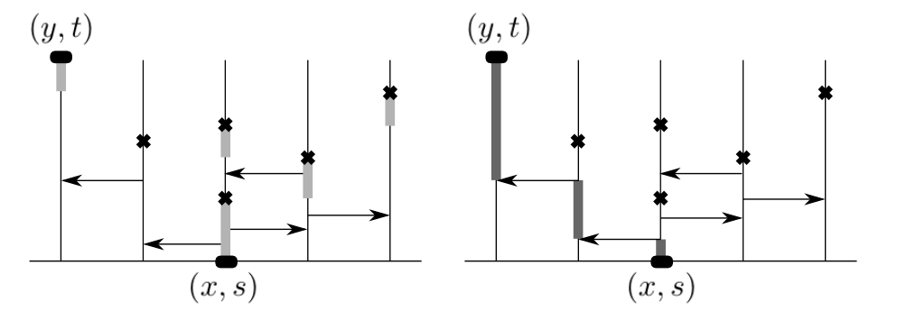
Refer to caption

Figure 3: Left: the thick gray trajectory represents the values of ηr(x,s)\eta^{(x,s)}_{r} for each r∈[s,t]r\in[s,t] (in order to identify this process, one can use the procedure mentioned after (4.2)). Right: the thick (darker) gray trajectory shows the unique RFBIP from (x,s)(x,s) to ℤ×{t}{\mathbb{Z}}\times\{t\}.

5.2 Introducing a drift: proof of Proposition 4.4

Our proof of Proposition 4.4 consists of two “ingredients”, each involving the definition of a random space-time point and the discussion of some of its properties. These ingredients are then combined to define the space-time point (𝒳,𝒯)(\mathcal{X},\mathcal{T}) of Proposition 4.4.

5.2.1 Ingredient 1: Bifurcation times of the ancestor process

We start our steering construction defining random times at which the ancestor process of (0,0)(0,0), (ηt)t≥0(\eta_{t})_{t\geq 0}, satisfies a list of conditions. The construction depends on a constant L∈ℕL\in\mathbb{N}, L>1L>1, which we will choose later.

In what follows, the word ‘arrow’ does not refer to selective arrows. Let t≥3t\geq 3 and assume that (0,0)↝ℤd×{t}(0,0)\rightsquigarrow{\mathbb{Z}}^{d}\times\{t\}, so that ηt≠△\eta_{t}\neq\triangle. Let y=ηt−3y=\eta_{t-3}. We say that tt is a bifurcation time of the ancestor process η\eta if we can find:

  • •

    no death mark in {y−e1,y,y+e1}×[t−3,t−1]\{y-e_{1},y,y+e_{1}\}\times[t-3,t-1];

  • •

    a death mark in {y}×[t−1,t]\{y\}\times[t-1,t];

  • •

    exactly two arrows started from {y}×[t−3,t−2]\{y\}\times[t-3,t-2]; one from yy to y+e1y+e_{1} and the other from yy to y−e1y-e_{1};

  • •

    no arrow started from {y}×[t−2,t]\{y\}\times[t-2,t];

  • •

    no arrow started from {y−e1,y+e1}×[t−3,t−1]\{y-e_{1},y+e_{1}\}\times[t-3,t-1];

  • •

    exactly one basic infection path from (y−e1,t−1)(y-e_{1},t-1) to ℤd×{t}{\mathbb{Z}}^{d}\times\{t\}, ending at y−L​e1y-Le_{1};

  • •

    exactly one basic infection path from (y+e1,t−1)(y+e_{1},t-1) to ℤd×{t}{\mathbb{Z}}^{d}\times\{t\}, ending at y+L​e1y+Le_{1}.

Note that bifurcation times depend on HH and not on ℋ\mathcal{H}. See Figure 4 for an illustration of a bifurcation time.

Refer to caption

Figure 4: Illustration of a bifurcation time tt of the ancestor process η\eta (in the d=1d=1 case).

We now want to find a bifurcation time tt around a spatial location yy with the property that (y−L​e1,t)↝∞(y-Le_{1},t)\rightsquigarrow\infty or (y+L​e1,t)↝∞(y+Le_{1},t)\rightsquigarrow\infty (or both). Let us first give an heuristic explanation to our approach to find such a point. We start following the ancestor process η\eta until a bifurcation time uu is found (the bifurcation occurs in the time interval [u−3,u][u-3,u], around a spatial location y=ηu−3y=\eta_{u-3}). We then ask if at least one of (y−L​e1,u)↝∞(y-Le_{1},u)\rightsquigarrow\infty and (y+L​e1,u)↝∞(y+Le_{1},u)\rightsquigarrow\infty holds. If the answer is affirmative, we are done with our search. Otherwise, we wait until the first time vv such that {(y−L​e1,u),(y+L​e1,u)}↝̸ℤd×{v}\{(y-Le_{1},u),(y+Le_{1},u)\}\not\rightsquigarrow{\mathbb{Z}}^{d}\times\{v\}; then we look for a new bifurcation time u′u^{\prime} after vv, and repeat the procedure.

We now give the rigorous description of this procedure. Let U1U_{1} be the smallest bifurcation time in HH (with the convention that U1=∞U_{1}=\infty if there is no bifurcation time). Note that U1U_{1} is a stopping time with respect to the natural filtration of the Poisson processes in HH. In the event {U1<∞}\{U_{1}<\infty\}, we let Y1=ηU1−3Y_{1}=\eta_{U_{1}-3}, that is, Y1Y_{1} is the spatial position around which the bifurcation at U1U_{1} occurs. Then define another stopping time V1V_{1} as:

V1={sup{t:{(Y1−L​e1,U1),(Y1+L​e1,U1)}↝ℤd×{t}}if ​U1<∞;∞otherwise.V_{1}=\begin{cases}\sup\{t:\{(Y_{1}-Le_{1},U_{1}),(Y_{1}+Le_{1},U_{1})\}\rightsquigarrow{\mathbb{Z}}^{d}\times\{t\}\}&\text{if }U_{1}<\infty;\\ \infty&\text{otherwise}.\end{cases}

In words, in case U1<∞U_{1}<\infty, V1V_{1} is the supremum of all times tt that can be reached by BIP’s γ:[U1,t]→ℤd\gamma:[U_{1},t]\to{\mathbb{Z}}^{d} with γ⁡(U1)∈{Y1−L​e1,Y1+L​e1}\gamma(U_{1})\in\{Y_{1}-Le_{1},Y_{1}+Le_{1}\}. Next, if V1<∞V_{1}<\infty, ηV1≠△\eta_{V_{1}}\neq\triangle and the ancestor process has at least one bifurcation time t≥V1+3t\geq V_{1}+3, we let U2U_{2} be the smallest bifurcation time larger than V1+3V_{1}+3, and let Y2=ηU2−3Y_{2}=\eta_{U_{2}-3}. In all other cases (that is, (a) if V1=∞V_{1}=\infty, (b) if V1<∞V_{1}<\infty but ηV1=△\eta_{V_{1}}=\triangle, or (c) if the ancestor process has no bifurcation time after V1+3V_{1}+3), we let U2=∞U_{2}=\infty and Y2=△Y_{2}=\triangle. Then, V2V_{2} is defined exactly as V1V_{1}, with U1,Y1U_{1},Y_{1} replaced by U2,Y2U_{2},Y_{2}. We then proceed similarly for other values of kk to obtain a sequence (Uk,Vk)(U_{k},V_{k}) with Uk≤Vk≤Uk+1U_{k}\leq V_{k}\leq U_{k+1} for each kk.

In case there exists k⋆{k_{\star}} for which Uk⋆<∞U_{k_{\star}}<\infty (so that there is a bifurcation connecting (Yk⋆,Uk⋆−3)(Y_{k_{\star}},U_{k_{\star}}-3) to the two points (Yk⋆−L​e1,Uk⋆)(Y_{k_{\star}}-Le_{1},U_{k_{\star}}) and (Yk⋆+L​e1,Uk⋆)(Y_{k_{\star}}+Le_{1},U_{k_{\star}})) and Vk⋆=∞V_{k_{\star}}=\infty (so that (Yk⋆−L​e1,Uk⋆)↝∞(Y_{k_{\star}}-Le_{1},U_{k_{\star}})\rightsquigarrow\infty or (Yk⋆+L​e1,Uk⋆)↝∞(Y_{k_{\star}}+Le_{1},U_{k_{\star}})\rightsquigarrow\infty, or both), we let U⋆=Uk⋆U_{\star}=U_{k_{\star}} and Y⋆=Yk⋆Y_{\star}=Y_{k_{\star}}. Otherwise, we let U⋆=∞U_{\star}=\infty and Y⋆=△Y_{\star}=\triangle.

We now state two lemmas that will be needed about these random times; the proofs are postponed to Section 6.1 in the Appendix.

Lemma 5.2.

Conditioned on {(0,0)↝∞}\{(0,0)\rightsquigarrow\infty\}, U⋆U_{\star} is almost surely finite:

ℙ[U⋆<∞∣(0,0)↝∞]=∑k=0∞ℙ[Uk<∞,Vk=∞∣(0,0)↝∞]=1.{\mathbb{P}}[U_{\star}<\infty\mid(0,0)\rightsquigarrow\infty]=\sum_{k=0}^{\infty}{\mathbb{P}}[U_{k}<\infty,\;V_{k}=\infty\mid(0,0)\rightsquigarrow\infty]=1. (5.2)

Moreover, there exists σ1>0\sigma_{1}>0 (depending on LL) such that

𝔼⁡[exp⁡(σ1⋅U⋆)∣(0,0)↝∞]<∞.{\mathbb{E}}\left[\exp(\sigma_{1}\cdot U_{\star})\mid(0,0)\rightsquigarrow\infty\right]<\infty. (5.3)
Lemma 5.3.

Given events E1,E2E_{1},E_{2} on Harris systems,

ℙ[ℍ[0,U⋆]∈E1,ℍ∘θ(Y⋆,U⋆)∈E2∣(0,0)↝∞]=ℙ[ℍ[0,U⋆]∈E1∣(0,0)↝∞]⋅ℙ[ℍ∈E2∣{(−L,0)↝∞}∪{(L,0)↝∞}].\begin{split}&{\mathbb{P}}\left[\mathbb{H}_{[0,U_{\star}]}\in E_{1},\;\mathbb{H}\circ\theta(Y_{\star},U_{\star})\in E_{2}\mid(0,0)\rightsquigarrow\infty\right]\\ &={\mathbb{P}}\left[\mathbb{H}_{[0,U_{\star}]}\in E_{1}\mid(0,0)\rightsquigarrow\infty\right]\cdot{\mathbb{P}}\left[\mathbb{H}\in E_{2}\mid\{(-L,0)\rightsquigarrow\infty\}\cup\{(L,0)\rightsquigarrow\infty\}\right].\end{split} (5.4)

5.2.2 Ingredient 2: Survival time for one ancestry out of a pair

The second ingredient in our construction is another random space-time point (Z⋆,W⋆)(Z_{\star},W_{\star}) obtained as a function of the augmented Harris system ℍ\mathbb{H} (again, it will depend on HH and not ℋ\mathcal{H}). The definition of this space-time point will refer to the same constant LL that was used in the previous subsection. For now we only assume L∈ℕL\in{\mathbb{N}} and L>1L>1, but Lemma 5.6 will require LL to be chosen large.

We assume a Harris system HH is given and define

W0≡0,Z0≡0,W1=sup{t:(L​e1,0)↝ℤd×{t}}.W_{0}\equiv 0,\qquad Z_{0}\equiv 0,\qquad W_{1}=\sup\{t:(Le_{1},0)\rightsquigarrow{\mathbb{Z}}^{d}\times\{t\}\}.

We then let

Z1={ηW1(−L​e1,0)if ​W1<∞;△otherwise,Z_{1}=\begin{cases}\eta^{(-Le_{1},0)}_{W_{1}}&\text{if }W_{1}<\infty;\\[5.69046pt] \triangle&\text{otherwise,}\end{cases}

and inductively, for k≥1k\geq 1,

Wk+1={sup{t:(Zk,Wk)↝ℤd×{t}}if Wk<∞,Zk≠△;∞otherwise,\displaystyle W_{k+1}=\begin{cases}\sup\{t:(Z_{k},W_{k})\rightsquigarrow{\mathbb{Z}}^{d}\times\{t\}\}&\text{if }W_{k}<\infty,\;Z_{k}\neq\triangle;\\[5.69046pt] \infty&\text{otherwise,}\end{cases}
Zk+1={ηWk+1(−L​e1,0)if ​Wk+1<∞,△otherwise.\displaystyle Z_{k+1}=\begin{cases}\eta^{(-Le_{1},0)}_{W_{k+1}}&\text{if }W_{k+1}<\infty,\\[5.69046pt] \triangle&\text{otherwise.}\end{cases}

Now, if (L​e1,0)↝∞(Le_{1},0)\rightsquigarrow\infty, so that W1=∞W_{1}=\infty, we define (Z⋆,W⋆)=(L​e1,0)(Z_{\star},W_{\star})=(Le_{1},0). If, on the other hand, there exists a (necessarily unique) k⋆≥1k_{\star}\geq 1 such that Wk⋆<∞W_{k_{\star}}<\infty, Zk⋆≠△Z_{k_{\star}}\neq\triangle and Wk⋆+1=∞W_{{k_{\star}}+1}=\infty (so that (Zk⋆,Wk⋆)↝∞(Z_{k_{\star}},W_{k_{\star}})\rightsquigarrow\infty), we let (Z⋆,W⋆)=(Zk⋆,Wk⋆)(Z_{\star},W_{\star})=(Z_{k_{\star}},W_{k_{\star}}). In all other cases, we simply put (Z⋆,W⋆)=(△,∞)(Z_{\star},W_{\star})=(\triangle,\infty). These definitions are illustrated in Figure 5.

Refer to caption

Figure 5: The space-time points (Zk,Wk)(Z_{k},W_{k}) and (Z⋆,W⋆)(Z_{\star},W_{\star}) (dimension one). The grey triangle with the infinity symbol indicates that (Z3,W3)↝∞(Z_{3},W_{3})\rightsquigarrow\infty.
Lemma 5.4.

Conditioned on {(Le1,0)↝∞}∪{(−Le1,0)↝∞}\{(Le_{1},0)\rightsquigarrow\infty\}\cup\{(-Le_{1},0)\rightsquigarrow\infty\}, W⋆W_{\star} is almost surely finite:

ℙ[W⋆<∞∣{(Le1,0)↝∞}∪{(−Le1,0)↝∞}]=ℙ[W⋆=0∣{(Le1,0)↝∞}∪{(−Le1,0)↝∞}]+∑k=1∞ℙ[W⋆=Wk<∞∣{(Le1,0)↝∞}∪{(−Le1,0)↝∞}]=1;\begin{split}&{\mathbb{P}}\left[W_{\star}<\infty\mid\{(Le_{1},0)\rightsquigarrow\infty\}\cup\{(-Le_{1},0)\rightsquigarrow\infty\}\right]\\[5.69046pt] &\hskip 56.9055pt={\mathbb{P}}\left[W_{\star}=0\mid\{(Le_{1},0)\rightsquigarrow\infty\}\cup\{(-Le_{1},0)\rightsquigarrow\infty\}\right]\\ &\hskip 71.13188pt+\sum_{k=1}^{\infty}{\mathbb{P}}\left[W_{\star}=W_{k}<\infty\mid\{(Le_{1},0)\rightsquigarrow\infty\}\cup\{(-Le_{1},0)\rightsquigarrow\infty\}\right]=1;\end{split} (5.5)

moreover, there exists a constant σ2>0\sigma_{2}>0, independent of LL, such that

𝔼[exp(σ2⋅W⋆)∣{(Le1,0)↝∞}∪{(−Le1,0)↝∞}]<∞.{\mathbb{E}}\left[\exp(\sigma_{2}\cdot W_{\star})\mid\{(Le_{1},0)\rightsquigarrow\infty\}\cup\{(-Le_{1},0)\rightsquigarrow\infty\}\right]<\infty. (5.6)

The proof of this result is similar to that of Lemma 5.2, only simpler, so we will omit it.

Lemma 5.5.

Given events E1E_{1} and E2E_{2} on Harris systems,

ℙ[ℍ[0,W⋆]∈E1,ℍ∘θ(Z⋆,W⋆)∈E2∣{(Le1,0)↝∞}∪{(−Le1,0)↝∞}]=ℙ[ℍ[0,W⋆]∈E1∣{(Le1,0)↝∞}∪{(−Le1,0)↝∞}]⋅ℙ[ℍ∈E2∣{(Le1,0)↝∞}∪{(−Le1,0)↝∞}].\begin{split}&{\mathbb{P}}\left[\mathbb{H}_{[0,W_{\star}]}\in E_{1},\;\mathbb{H}\circ\theta(Z_{\star},W_{\star})\in E_{2}\mid\{(Le_{1},0)\rightsquigarrow\infty\}\cup\{(-Le_{1},0)\rightsquigarrow\infty\}\right]\\[5.69046pt] &={\mathbb{P}}\left[\mathbb{H}_{[0,W_{\star}]}\in E_{1}\mid\{(Le_{1},0)\rightsquigarrow\infty\}\cup\{(-Le_{1},0)\rightsquigarrow\infty\}\right]\\[5.69046pt] &\hskip 128.0374pt\cdot{\mathbb{P}}\left[\mathbb{H}\in E_{2}\mid\{(Le_{1},0)\rightsquigarrow\infty\}\cup\{(-Le_{1},0)\rightsquigarrow\infty\}\right].\end{split}

Lemma 5.5 is proved in Section 6.1 in the Appendix.

Lemma 5.6.

If LL is large enough,

𝔼[Z⋆∣{(Le1,0)↝∞}∪{(−Le1,0)↝∞}]=αL⋅e1,{{\mathbb{E}}}[Z_{\star}\mid\{(Le_{1},0)\rightsquigarrow\infty\}\cup\{(-Le_{1},0)\rightsquigarrow\infty\}]=\alpha_{L}\cdot e_{1},

where αL>0\alpha_{L}>0.

Proof.

We abbreviate

A−={(−Le1,0)↝∞},A+={(Le1,0)↝∞},A=A−∪A+.A_{-}=\{(-Le_{1},0)\rightsquigarrow\infty\},\qquad A_{+}=\{(Le_{1},0)\rightsquigarrow\infty\},\qquad A=A_{-}\cup A_{+}.

We first need to prove that

𝔼⁡[‖Z⋆‖⋅𝟙A]<∞.{\mathbb{E}}\left[\|Z_{\star}\|\cdot\mathds{1}_{A}\right]<\infty. (5.7)

To this end, we write A=A+∪(A+c∩A−)A=A_{+}\cup(A_{+}^{c}\cap A_{-}), so

Z⋆⋅𝟙A=L​e1⋅𝟙A+−L​e1⋅𝟙A+c∩A−+(Z⋆+L​e1)⋅𝟙A+c∩A−.\begin{split}&Z_{\star}\cdot\mathds{1}_{A}=Le_{1}\cdot\mathds{1}_{A_{+}}-Le_{1}\cdot\mathds{1}_{A_{+}^{c}\cap A_{-}}+(Z_{\star}+Le_{1})\cdot\mathds{1}_{A^{c}_{+}\cap A_{-}}.\end{split} (5.8)

Because of this equality, (5.7) will follow from the statement:

∃C>0:∀L>0,𝔼⁡[‖Z⋆+L​e1‖⋅𝟙A+c∩A−]<C.\exists C>0:\;\forall L>0,\;\;{\mathbb{E}}\left[\|Z_{\star}+Le_{1}\|\cdot\mathds{1}_{A_{+}^{c}\cap A_{-}}\right]<C. (5.9)

Let us prove (5.9). The expectation is equal to

𝔼⁡[‖ηW⋆(−L​e1,0)+L​e1‖⋅𝟙A+c∩A−].{\mathbb{E}}\left[\left\|\eta^{(-Le_{1},0)}_{W_{\star}}+Le_{1}\right\|\cdot\mathds{1}_{A_{+}^{c}\cap A_{-}}\right].

Define

Mt=sup{∥z+Le1∥:z∈ℤd,∃s≤t:(−Le1,0)↝(z,s)},t≥0.M_{t}=\sup\{\|z+Le_{1}\|:\;z\in{\mathbb{Z}}^{d},\;\exists s\leq t:\;(-Le_{1},0)\rightsquigarrow(z,s)\},\quad t\geq 0.

For any x>0x>0 and α∈(0,1)\alpha\in(0,1) we have

ℙ[‖η(−L​e1,0)W⋆+Le1‖⋅𝟙A+c∩A−>x]≤ℙ[{W⋆>αx}∩A+c∩A−]+ℙ[Mα​x>x].\begin{split}{\mathbb{P}}\left[\left\|\eta^{(-Le_{1},0)}_{W_{\star}}+Le_{1}\right\|\cdot\mathds{1}_{A_{+}^{c}\cap A_{-}}>x\right]\leq&{\mathbb{P}}\left[\{W_{\star}>\alpha x\}\cap A_{+}^{c}\cap A_{-}\right]+{\mathbb{P}}\left[M_{\alpha x}>x\right].\end{split} (5.10)

Using (5.6) and the Chebyshev’s inequality,

ℙ[{W⋆>αx}∩A+c∩A−]≤ℙ[{W⋆>αx}∩A+c∩A−∣A]≤ℙ⁡[W⋆>α​x∣A]<C​exp⁡(−σ2​α​x),\begin{split}{\mathbb{P}}\left[\{W_{\star}>\alpha x\}\cap A_{+}^{c}\cap A_{-}\right]&\leq{\mathbb{P}}\left[\{W_{\star}>\alpha x\}\cap A_{+}^{c}\cap A_{-}\mid A\right]\\ &\leq{\mathbb{P}}\left[W_{\star}>\alpha x\mid A\right]<C\exp(-\sigma_{2}\alpha x),\end{split} (5.11)

where CC is a constant that does not depend on LL. Next, by (2.3),

ℙ[Mα​x>x]≤exp(b1αx−b2x).{\mathbb{P}}\left[M_{\alpha x}>x\right]\leq\exp(b_{1}\alpha x-b_{2}x). (5.12)

Using (5.11) and (5.12) in (5.10) with α<b2/b1\alpha<b_{2}/b_{1} and integrating over xx, we obtain (5.9), so also (5.7).

By symmetry, we have 𝔼⁡[Z⋆⋅ei]=0\mathbb{E}[Z_{\star}\cdot e_{i}]=0 for all i≠1i\neq 1. To treat the expectation of Z⋆⋅e1Z_{\star}\cdot e_{1}, we use (5.8) to decompose:

𝔼⁡[(Z⋆⋅e1)​𝟙A]\displaystyle{\mathbb{E}}\left[(Z_{\star}\cdot e_{1})\mathds{1}_{A}\right]
=L⋅ℙ⁡(A+)−L⋅ℙ⁡(A+c∩A−)+𝔼⁡[(Z⋆⋅e1+L)⋅𝟙A+c∩A−]\displaystyle=L\cdot{\mathbb{P}}(A_{+})-L\cdot{\mathbb{P}}(A_{+}^{c}\cap A_{-})+{\mathbb{E}}\left[(Z_{\star}\cdot e_{1}+L)\cdot\mathds{1}_{A_{+}^{c}\cap A_{-}}\right]
=L⋅ℙ⁡(A+)−L⋅ℙ⁡(A+∩A−c)+𝔼⁡[(Z⋆⋅e1+L)⋅𝟙A+c∩A−]\displaystyle=L\cdot{\mathbb{P}}(A_{+})-L\cdot{\mathbb{P}}(A_{+}\cap A_{-}^{c})+{\mathbb{E}}\left[(Z_{\star}\cdot e_{1}+L)\cdot\mathds{1}_{A_{+}^{c}\cap A_{-}}\right]
=L⋅ℙ⁡[A+∩A−]+𝔼⁡[(Z⋆⋅e1+L)⋅𝟙A+c∩A−]\displaystyle=L\cdot{\mathbb{P}}[A_{+}\cap A_{-}]+{\mathbb{E}}\left[(Z_{\star}\cdot e_{1}+L)\cdot\mathds{1}_{A_{+}^{c}\cap A_{-}}\right]
≥L⋅ℙ[(0,0)↝∞]2+𝔼[(Z⋆⋅e1+L)⋅𝟙A+c∩A−]\displaystyle\geq L\cdot{\mathbb{P}}[(0,0)\rightsquigarrow\infty]^{2}+{\mathbb{E}}\left[(Z_{\star}\cdot e_{1}+L)\cdot\mathds{1}_{A_{+}^{c}\cap A_{-}}\right]

where the last step follows from the FKG inequality and translation invariance. By (5.9), we can now choose LL large enough that the right-hand side is positive, completing the proof.  

We end this subsection defining (Zk′,Wk′)k≥0,(Z⋆′,W⋆′)(Z_{k}^{\prime},W_{k}^{\prime})_{k\geq 0},\;(Z_{\star}^{\prime},W_{\star}^{\prime}) exactly as (Zk,Wk)k≥1,(Z⋆,W⋆)(Z_{k},W_{k})_{k\geq 1},\;(Z_{\star},W_{\star}), but inverting the roles of L​e1Le_{1} and −L​e1-Le_{1}. More formally, we define

(Zk′,Wk′)=(Zk,Wk)∘ψ1,−1,(Z⋆′,W⋆′)=(Z⋆,W⋆)∘ψ1,−1(Z_{k}^{\prime},W_{k}^{\prime})=(Z_{k},W_{k})\circ\psi^{1,-1},\qquad(Z_{\star}^{\prime},W_{\star}^{\prime})=(Z_{\star},W_{\star})\circ\psi^{1,-1}

where ψ1,−1\psi^{1,-1} is as defined in (4.5), that is, it is the linear transformation ψ1,−1​(x1,x2,…,xd)=(−x1,x2,…,xd)\psi^{1,-1}(x_{1},x_{2},\ldots,x_{d})=(-x_{1},x_{2},\ldots,x_{d}). Choosing LL large enough as required by Lemma 5.6, we then have

𝔼[Z⋆′∣{(−Le1,0)↝∞}∪{(Le1,0)↝∞}]=−αLe1.{{\mathbb{E}}}[Z_{\star}^{\prime}\mid\{(-Le_{1},0)\rightsquigarrow\infty\}\cup\{(Le_{1},0)\rightsquigarrow\infty\}]=-\alpha_{L}e_{1}. (5.13)

5.2.3 Putting ingredients together

In what follows, we always assume that the event {(0,0)↝∞}\{(0,0)\rightsquigarrow\infty\} occurs. By Lemma 5.2, it follows from this assumption that U⋆<∞U_{\star}<\infty, Y⋆∈ℤdY_{\star}\in\mathbb{Z}^{d}.

Recall that, if U⋆U_{\star} is a bifurcation time, then there is exactly one arrow from {Y⋆}×[U⋆−3,U⋆−2]\{Y_{\star}\}\times[U_{\star}-3,U_{\star}-2] to {Y⋆−e1}×[U⋆−3,U⋆−2]\{Y_{\star}-e_{1}\}\times[U_{\star}-3,U_{\star}-2] and one arrow from {Y⋆}×[U⋆−3,U⋆−2]\{Y_{\star}\}\times[U_{\star}-3,U_{\star}-2] to {Y⋆+e1}×[U⋆−3,U⋆−2]\{Y_{\star}+e_{1}\}\times[U_{\star}-3,U_{\star}-2]. Let t(−),t(+)∈[U⋆−3,U⋆−2]t_{(-)},t_{(+)}\in[U_{\star}-3,U_{\star}-2] be the respective times at which these arrows are present. Define

E={for some t∈[U⋆−2,U⋆−1], there is a selective arrow from (Y⋆,t) to (Y⋆+e1,t)}.E=\left\{\text{for some $t\in[U_{\star}-2,U_{\star}-1]$, there is a selective arrow from $(Y_{\star},t)$ to $(Y_{\star}+e_{1},t)$}\right\}.

If EE occurs, let t(+)′∈[U⋆−2,U⋆−1]t_{(+)}^{\prime}\in[U_{\star}-2,U_{\star}-1] be the first time in [U⋆−2,U⋆−1][U_{\star}-2,U_{\star}-1] at which a selective arrow as mentioned in EE appears.

We now define the random variables 𝒯\mathcal{T} and 𝒳\mathcal{X} in the statement of Proposition 4.4:

(𝒳,𝒯)={(Y⋆,U⋆)+(Z⋆,W⋆)∘θ⁡(Y⋆,U⋆)on E∪{t(+)>t(−)};(Y⋆,U⋆)+(Z⋆′,W⋆′)∘θ⁡(Y⋆,U⋆)on Ec∩{t(+)<t(−)}.\displaystyle(\mathcal{X},\mathcal{T})=\begin{cases}(Y_{\star},U_{\star})+(Z_{\star},W_{\star})\circ\theta(Y_{\star},U_{\star})&\text{on }E\cup\{t_{(+)}>t_{(-)}\};\\[5.69046pt] (Y_{\star},U_{\star})+(Z^{\prime}_{\star},W^{\prime}_{\star})\circ\theta(Y_{\star},U_{\star})&\text{on }E^{c}\cap\{t_{(+)}<t_{(-)}\}.\end{cases} (5.14)
Proof of Proposition 4.4(1).

We will construct an RFSIP γ⋆:[0,𝒯]→ℤd\upgamma_{\star}:[0,\mathcal{T}]\to{\mathbb{Z}}^{d} with γ⋆​(0)=0\upgamma_{\star}(0)=0 and γ⋆​(𝒯)=𝒳\upgamma_{\star}(\mathcal{T})=\mathcal{X}. The definition of γ⋆\upgamma_{\star} will be split into six cases. In each case, it will be straightforward to verify that γ⋆\upgamma_{\star} is either an RFBIP (cases 1-4 and 6) or an RFSIP (case 5). Figure 6 serves as a useful guide to the construction.

In all cases, on [0,U⋆−3][0,U_{\star}-3] we let γ⋆\upgamma_{\star} be equal to the unique RFBIP from (0,0)(0,0) to (Y⋆,U⋆−3)(Y_{\star},U_{\star}-3) (such an RFBIP exists by the definition of the ancestor process, since ηU⋆−3=Y⋆\eta_{U_{\star}-3}=Y_{\star}).

Refer to caption

Figure 6: The six cases in the definition of the RFSIP γ⋆\upgamma_{\star} from (0,0)(0,0) to (𝒳,𝒯)(\mathcal{X},\mathcal{T}) (dimension one). The path γ⋆\upgamma_{\star} is shown as a thick grey line. A grey triangle with the infinity sign at a space-time point (x,t)(x,t) indicates that (x,t)↝∞(x,t)\rightsquigarrow\infty. In each case one verifies that γ⋆\upgamma_{\star} is an RFSIP because whenever it jumps, that is, whenever γ⋆​(t−)=x≠y=γ⋆​(t)\upgamma_{\star}(t-)=x\neq y=\upgamma_{\star}(t), we have (x,t+)↝̸𝒯(x,t+)\not\rightsquigarrow\mathcal{T}.
  • Case 1:

    Ec∩{t(−)>t(+)}∩{(Y⋆−Le1,U⋆)↝∞}E^{c}\cap\{t_{(-)}>t_{(+)}\}\cap\{(Y_{\star}-Le_{1},U_{\star})\rightsquigarrow\infty\} occurs. In this case, we have

    (𝒳,𝒯)=(Y⋆,U⋆)+(Z⋆′,W⋆′)∘θ⁡(Y⋆,U⋆)(\mathcal{X},\mathcal{T})=(Y_{\star},U_{\star})+(Z^{\prime}_{\star},W^{\prime}_{\star})\circ\theta(Y_{\star},U_{\star}) (5.15)

    and in the translated Harris system H∘θ⁡(Y⋆,U⋆)H\circ\theta(Y_{\star},U_{\star}) we have (−L​e1,0)↝∞(-Le_{1},0)\rightsquigarrow\infty and hence W⋆′∘θ⁡(Y⋆,U⋆)=0W^{\prime}_{\star}\circ\theta(Y_{\star},U_{\star})=0 and Z⋆′∘θ⁡(Y⋆,U⋆)=−L​e1Z^{\prime}_{\star}\circ\theta(Y_{\star},U_{\star})=-Le_{1}. Hence, (𝒳,𝒯)=(Y⋆−L​e1,U⋆)(\mathcal{X},\mathcal{T})=(Y_{\star}-Le_{1},U_{\star}). Then, we set:

    • ∙\bullet

      on [U⋆−3,t(−))[U_{\star}-3,\;t_{(-)}), γ⋆\upgamma_{\star} equal to Y⋆Y_{\star};

    • ∙\bullet

      on [t(−),U⋆]=[t(−),𝒯][t_{(-)},\;U_{\star}]=[t_{(-)},\;\mathcal{T}], γ⋆\upgamma_{\star} equal to the unique RFBIP from (Y⋆−e1,t(−))(Y_{\star}-e_{1},\;t_{(-)}) to (Y⋆−L​e1,U⋆)(Y_{\star}-Le_{1},\;U_{\star}).

  • Case 2:

    Ec∩{t(−)>t(+)}∩{(Y⋆−Le1,U⋆)↝̸∞}E^{c}\cap\{t_{(-)}>t_{(+)}\}\cap\{(Y_{\star}-Le_{1},U_{\star})\not\rightsquigarrow\infty\} occurs. We again have (5.15), but now W⋆′∘θ⁡(Y⋆,U⋆)>0W^{\prime}_{\star}\circ\theta(Y_{\star},U_{\star})>0, so that 𝒯>U⋆\mathcal{T}>U_{\star}, and 𝒳=η𝒯(Y⋆+L​e1,U⋆)\mathcal{X}=\eta^{(Y_{\star}+Le_{1},U_{\star})}_{\mathcal{T}}, by the definition of Z⋆′Z^{\prime}_{\star}. In particular, there is a unique RFBIP from (Y⋆+L​e1,U⋆)(Y_{\star}+Le_{1},U_{\star}) to (𝒳,𝒯)(\mathcal{X},\mathcal{T}). We set

    • ∙\bullet

      on [U⋆−3,t(+))[U_{\star}-3,\;t_{(+)}), γ⋆\upgamma_{\star} equal to Y⋆Y_{\star};

    • ∙\bullet

      on [t(+),U⋆)[t_{(+)},\;U_{\star}), γ⋆\upgamma_{\star} equal to the unique RFBIP from (Y⋆+e1,t(+))(Y_{\star}+e_{1},\;t_{(+)}) to (Y⋆+L​e1,U⋆)(Y_{\star}+Le_{1},\;U_{\star});

    • ∙\bullet

      on [U⋆,𝒯][U_{\star},\mathcal{T}], γ⋆\upgamma_{\star} equal to the unique RFBIP from (Y⋆+L​e1,U⋆)(Y_{\star}+Le_{1},U_{\star}) to (𝒳,𝒯)(\mathcal{X},\mathcal{T}).

  • Case 3:

    Ec∩{t(+)>t(−)}∩{(Y⋆+Le1,U⋆)↝∞}E^{c}\cap\{t_{(+)}>t_{(-)}\}\cap\{(Y_{\star}+Le_{1},U_{\star})\rightsquigarrow\infty\} occurs. We have

    (𝒳,𝒯)=(Y⋆,U⋆)+(Z⋆,W⋆)∘θ⁡(Y⋆,U⋆)(\mathcal{X},\mathcal{T})=(Y_{\star},U_{\star})+(Z_{\star},W_{\star})\circ\theta(Y_{\star},U_{\star}) (5.16)

    and in the translated Harris system H∘θ⁡(Y⋆,U⋆)H\circ\theta(Y_{\star},U_{\star}) we have (L​e1,0)↝∞(Le_{1},0)\rightsquigarrow\infty, so (𝒳,𝒯)=(Y⋆+L​e1,U⋆)(\mathcal{X},\mathcal{T})=(Y_{\star}+Le_{1},U_{\star}). We set:

    • ∙\bullet

      on [U⋆−3,t(+))[U_{\star}-3,\;t_{(+)}), γ⋆\upgamma_{\star} equal to Y⋆Y_{\star};

    • ∙\bullet

      on [t(+),U⋆]=[t(+),𝒯][t_{(+)},\;U_{\star}]=[t_{(+)},\;\mathcal{T}], γ⋆\upgamma_{\star} equal to the unique RFBIP from (Y⋆+e1,t(+))(Y_{\star}+e_{1},\;t_{(+)}) to (Y⋆+L​e1,U⋆)(Y_{\star}+Le_{1},\;U_{\star}).

  • Case 4:

    Ec∩{t(+)>t(−)}∩{(Y⋆+Le1,U⋆)↝̸∞}E^{c}\cap\{t_{(+)}>t_{(-)}\}\cap\{(Y_{\star}+Le_{1},U_{\star})\not\rightsquigarrow\infty\} occurs. We again have (5.16), but now 𝒯\mathcal{T} is some time larger than U⋆U_{\star} and 𝒳=η𝒯(Y⋆−L​e1,U⋆)\mathcal{X}=\eta^{(Y_{\star}-Le_{1},U_{\star})}_{\mathcal{T}}. We set:

    • ∙\bullet

      on [U⋆−3,t(−))[U_{\star}-3,\;t_{(-)}), γ⋆\upgamma_{\star} equal to Y⋆Y_{\star};

    • ∙\bullet

      on [t(−),U⋆)[t_{(-)},\;U_{\star}), γ⋆\upgamma_{\star} equal to the unique RFBIP from (Y⋆−e1,t(−))(Y_{\star}-e_{1},\;t_{(-)}) to (Y⋆−L​e1,U⋆)(Y_{\star}-Le_{1},\;U_{\star});

    • ∙\bullet

      on [U⋆,𝒯][U_{\star},\mathcal{T}], γ⋆\upgamma_{\star} equal to the unique RFBIP from (Y⋆−L​e1,U⋆)(Y_{\star}-Le_{1},U_{\star}) to (𝒳,𝒯)(\mathcal{X},\mathcal{T}).

  • Case 5:

    E∩{(Y⋆+Le1,U⋆)↝∞}E\cap\{(Y_{\star}+Le_{1},U_{\star})\rightsquigarrow\infty\}. In this case we again have (5.16). We define γ⋆\upgamma_{\star} as in Case 3, with the only difference that we replace t(+)t_{(+)} by t(+)′t_{(+)}^{\prime} everywhere.

  • Case 6:

    E∩{(Y⋆+Le1,U⋆)↝̸∞}E\cap\{(Y_{\star}+Le_{1},U_{\star})\not\rightsquigarrow\infty\}. As in Case 4, we have (5.16) with 𝒯>U⋆\mathcal{T}>U_{\star} and 𝒳=η𝒯(Y⋆−L​e1,U⋆)\mathcal{X}=\eta^{(Y_{\star}-Le_{1},U_{\star})}_{\mathcal{T}}. We define γ⋆\upgamma_{\star} exactly as in Case 4.


Proof of Proposition 4.4(2)-(4).

Statement (2) follows directly from Lemmas 5.3 and 5.5. The fact that

𝔼⁡[exp⁡(σ​𝒯)∣(0,0)↝∞]<∞\mathbb{E}\left[\exp(\sigma\mathcal{T})\mid(0,0)\rightsquigarrow\infty\right]<\infty

if σ\sigma is small enough follows from (5.3), Lemma 5.3 and (5.6). Now, let

Mt=sup{∥x∥:x∈ℤd,there is an SIP from (0,0) to (x,s) for some s≤t},t≥0.M_{t}=\sup\{\|x\|:x\in{\mathbb{Z}}^{d},\;\text{there is an SIP from $(0,0)$ to $(x,s)$ for some }s\leq t\},\quad t\geq 0.

Noting that there is an SIP from (0,0)(0,0) to (𝒳,𝒯)(\mathcal{X},\mathcal{T}) we have, for any α∈(0,1)\alpha\in(0,1) and x>0x>0,

ℙ[𝒳⋅𝟙{(0,0)↝∞}>x]≤\displaystyle\mathbb{P}\left[\mathcal{X}\cdot\mathds{1}_{\{(0,0)\rightsquigarrow\infty\}}>x\right]\leq ℙ[(0,0)↝∞,𝒯>αx]+ℙ[Mα​x>x].\displaystyle{\mathbb{P}}\left[(0,0)\rightsquigarrow\infty,\;\mathcal{T}>\alpha x\right]+{\mathbb{P}}\left[M_{\alpha x}>x\right].

We can then bound the two terms on the right-hand side as we did in (5.11) and (5.12) to show that, if σ\sigma is small enough,

𝔼⁡[exp⁡(σ​𝒳)∣(0,0)↝∞]<∞.\mathbb{E}\left[\exp(\sigma\mathcal{X})\mid(0,0)\rightsquigarrow\infty\right]<\infty.

Hence, (3) is proved.

We now turn to (4). We abbreviate

ℙ~(⋅)=ℙ(⋅∣(0,0)↝∞),𝔼~(⋅)=𝔼(⋅∣(0,0)↝∞),\displaystyle\widetilde{\mathbb{P}}(\cdot)=\mathbb{P}(\cdot\mid(0,0)\rightsquigarrow\infty),\quad\widetilde{\mathbb{E}}(\cdot)=\mathbb{E}(\cdot\mid(0,0)\rightsquigarrow\infty),
𝔼^(⋅)=𝔼(⋅∣{(−Le1,0)↝∞}∪{(Le1,0)↝∞}).\displaystyle\widehat{\mathbb{E}}(\cdot)=\mathbb{E}(\cdot\mid\{(-Le_{1},0)\rightsquigarrow\infty\}\cup\{(Le_{1},0)\rightsquigarrow\infty\}).

We start with the equalities

𝔼~[𝟙E∪{t(+)>t(−)}⋅𝒳]=(5.14)𝔼~[𝟙E∪{t(+)>t(−)}⋅(Y⋆+Z⋆∘θ(Y⋆,U⋆))]=(5.4)𝔼~[𝟙E∪{t(+)>t(−)}⋅Y⋆]+ℙ~[E∪{t(+)>t(−)}]⋅𝔼^[Z⋆];\begin{split}\widetilde{{\mathbb{E}}}[\mathds{1}_{E\cup\{t_{(+)}>t_{(-)}\}}\cdot\mathcal{X}]&\stackrel{{\scriptstyle\eqref{eq:def_of_final_rvs}}}{{=}}\widetilde{{\mathbb{E}}}[\mathds{1}_{E\cup\{t_{(+)}>t_{(-)}\}}\cdot(Y_{\star}+Z_{\star}\circ\theta(Y_{\star},U_{\star}))]\\[5.69046pt] &\stackrel{{\scriptstyle\eqref{eq:distr_ingr_1}}}{{=}}\widetilde{{\mathbb{E}}}[\mathds{1}_{E\cup\{t_{(+)}>t_{(-)}\}}\cdot Y_{\star}]+\widetilde{{\mathbb{P}}}[E\cup\{t_{(+)}>t_{(-)}\}]\cdot\widehat{{\mathbb{E}}}[Z_{\star}];\end{split} (5.17)
𝔼~[𝟙Ec∩{t(+)<t(−)}⋅𝒳]=(5.14)𝔼~[𝟙Ec∩{t(+)<t(−)}⋅(Y⋆+Z′⋆∘θ(Y⋆,U⋆))]=(5.4)𝔼~[𝟙Ec∩{t(+)<t(−)}⋅Y⋆]+ℙ~[Ec∩{t(+)<t(−)}]⋅𝔼^[Z′⋆];\begin{split}\widetilde{{\mathbb{E}}}[\mathds{1}_{E^{c}\cap\{t_{(+)}<t_{(-)}\}}\cdot\mathcal{X}]&\stackrel{{\scriptstyle\eqref{eq:def_of_final_rvs}}}{{=}}\widetilde{{\mathbb{E}}}[\mathds{1}_{E^{c}\cap\{t_{(+)}<t_{(-)}\}}\cdot(Y_{\star}+Z^{\prime}_{\star}\circ\theta(Y_{\star},U_{\star}))]\\[5.69046pt] &\stackrel{{\scriptstyle\eqref{eq:distr_ingr_1}}}{{=}}\widetilde{{\mathbb{E}}}[\mathds{1}_{E^{c}\cap\{t_{(+)}<t_{(-)}\}}\cdot Y_{\star}]+\widetilde{{\mathbb{P}}}[E^{c}\cap\{t_{(+)}<t_{(-)}\}]\cdot\widehat{{\mathbb{E}}}[Z^{\prime}_{\star}];\end{split} (5.18)

By symmetry, 𝔼~​[Y⋆]=0\widetilde{{\mathbb{E}}}[Y_{\star}]=0 and 𝔼^​[Z⋆]=−𝔼^​[Z⋆′]\widehat{{\mathbb{E}}}[Z_{\star}]=-\widehat{{\mathbb{E}}}[Z^{\prime}_{\star}], so adding together (5.17) and (5.18) yields

𝔼~[𝒳]=𝔼^[Z⋆]⋅(ℙ~[E∪{t(+)>t(−)}]−ℙ~[Ec∩{t(+)<t(−)}]).\widetilde{{\mathbb{E}}}[\mathcal{X}]=\widehat{{\mathbb{E}}}[Z_{\star}]\cdot(\widetilde{{\mathbb{P}}}[E\cup\{t_{(+)}>t_{(-)}\}]-\widetilde{{\mathbb{P}}}[E^{c}\cap\{t_{(+)}<t_{(-)}\}]). (5.19)

Noting that EE only depends on the presence of a selective arrow on [U⋆−2,U⋆−1][U_{\star}-2,U_{\star}-1] and again using symmetry, we have

ℙ~[Ec∩{t(+)<t(−)}]=e−(λ1−λ2)⋅ℙ~[t(+)<t(−)]=12⋅e−(λ1−λ2)<12\displaystyle\widetilde{{\mathbb{P}}}[E^{c}\cap\{t_{(+)}<t_{(-)}\}]=e^{-(\lambda_{1}-\lambda_{2})}\cdot\widetilde{{\mathbb{P}}}[t_{(+)}<t_{(-)}]=\frac{1}{2}\cdot e^{-(\lambda_{1}-\lambda_{2})}<\frac{1}{2}
⟹ℙ~[E∪{t(+)>t(−)}]>12.\displaystyle\hskip 199.16928pt\Longrightarrow\quad\widetilde{{\mathbb{P}}}[E\cup\{t_{(+)}>t_{(-)}\}]>\frac{1}{2}.

Using this and the fact that 𝔼^​[Z⋆]>0\widehat{{\mathbb{E}}}[Z_{\star}]>0 in (5.19) concludes the proof.  

6 Appendix

6.1 Proofs of results of Section 5

We let (ℱt)t≥0(\mathscr{F}_{t})_{t\geq 0} denote the natural filtration of the Poisson point processes in ℍ\mathbb{H} (that is, for each tt, ℱt\mathscr{F}_{t} is the σ\sigma-algebra generated by ℍ[0,t]\mathbb{H}_{[0,t]}). Before turning to the statements of Section 5, we state and prove a preliminary result.

Lemma 6.1.

There exists σ0>0\sigma_{0}>0 such that

𝔼[exp(σ0U1)⋅𝟙{U1<∞}]<∞\mathbb{E}\left[\exp({\sigma_{0}U_{1}})\cdot\mathds{1}_{\{U_{1}<\infty\}}\right]<\infty (6.1)

and, for any kk, on {Vk<∞,ηVk≠△}\{V_{k}<\infty,\;\eta_{V_{k}}\neq\triangle\},

𝔼[exp(σ0(Uk+1−Vk))⋅𝟙{Uk+1<∞}∣ℱVk]<∞.\mathbb{E}\left[\exp({\sigma_{0}(U_{k+1}-V_{k})})\cdot\mathds{1}_{\{U_{k+1}<\infty\}}\mid\mathscr{F}_{V_{k}}\right]<\infty. (6.2)
Proof.

Let ℰ\mathcal{E} be the set of augmented Harris systems for which t=3t=3 is a bifurcation time. We have ℙ⁡(ℰ)>0{\mathbb{P}}(\mathcal{E})>0, since the occurrence of ℰ\mathcal{E} can be guaranteed by making prescriptions on finitely many Poisson processes on the time interval [0,3][0,3].

For t≥3t\geq 3, we have

ℙ⁡[ηt≠△,U1>t]\displaystyle{\mathbb{P}}\left[\eta_{t}\neq\triangle,\;U_{1}>t\right] ≤ℙ[ηt−3≠△,U1>t−3,ℍ∘θ(ηt−3,t−3)∉ℰ]\displaystyle\leq{\mathbb{P}}\left[\eta_{t-3}\neq\triangle,\;U_{1}>t-3,\;\mathbb{H}\circ\theta(\eta_{t-3},t-3)\notin\mathcal{E}\right]
=ℙ⁡[ηt−3≠△,U1>t−3]⋅ℙ⁡(ℰc),\displaystyle={\mathbb{P}}\left[\eta_{t-3}\neq\triangle,\;U_{1}>t-3\right]\cdot{\mathbb{P}}(\mathcal{E}^{c}),

and iterating we show that the right-hand side is less than ℙ​(ℰc)⌊t/3⌋{\mathbb{P}}(\mathcal{E}^{c})^{\lfloor t/3\rfloor}, proving that, if c>0c>0 is small enough,

ℙ⁡[ηt≠△,U1>t]<e−c​t,t≥3.{\mathbb{P}}\left[\eta_{t}\neq\triangle,\;U_{1}>t\right]<e^{-ct},\qquad t\geq 3. (6.3)

Then, noting that {U1<∞}⊆{ηt≠△∀t<U1}\{U_{1}<\infty\}\subseteq\{\eta_{t}\neq\triangle\;\forall t<U_{1}\},

𝔼[eσ​U1⋅𝟙{U1<∞}]\displaystyle{\mathbb{E}}\left[e^{\sigma U_{1}}\cdot\mathds{1}_{\{U_{1}<\infty\}}\right] =∫0∞ℙ[eσ​U1⋅𝟙{U1<∞}>x]𝖽x\displaystyle=\int_{0}^{\infty}{\mathbb{P}}\left[e^{\sigma U_{1}}\cdot\mathds{1}_{\{U_{1}<\infty\}}>x\right]\mathsf{d}x
≤∫0∞ℙ[U1>log⁡(x)σ,ηt≠△∀t<U1]𝖽x≤(6.3)∫0∞e−cσ​log⁡(x)𝖽x<∞\displaystyle\leq\int_{0}^{\infty}{\mathbb{P}}\left[U_{1}>\frac{\log(x)}{\sigma},\;\eta_{t}\neq\triangle\;\forall t<U_{1}\right]\mathsf{d}x\stackrel{{\scriptstyle\eqref{eq:behavior_U_init}}}{{\leq}}\int_{0}^{\infty}e^{-\frac{c}{\sigma}\log(x)}\mathsf{d}x<\infty

if σ∈(0,c)\sigma\in(0,c).

To prove (6.2), we argue as above (also using the strong Markov property with respect to the stopping time VkV_{k}) to obtain that, for any kk, on the event {Vk<∞,ηVk≠△}\{V_{k}<\infty,\;\eta_{V_{k}}\neq\triangle\},

ℙ[ηVk+t≠△,Uk+1>Vk+t∣ℱVk]<e−c​t,t>0;{\mathbb{P}}\left[\eta_{V_{k}+t}\neq\triangle,\;U_{k+1}>V_{k}+t\mid\mathscr{F}_{V_{k}}\right]<e^{-ct},\qquad t>0; (6.4)

we then complete the proof as above.  

Proof of Lemma 5.2.

To prove (5.2), start noting that, for all k≥1k\geq 1,

ℙ[Uk+1=∞∣Vk<∞,(0,0)↝∞]\displaystyle{\mathbb{P}}\left[U_{k+1}=\infty\mid V_{k}<\infty,\;(0,0)\rightsquigarrow\infty\right]
=ℙ[(0,0)↝∞,Vk<∞]−1limt→∞ℙ[(0,0)↝∞,Vk<∞,Uk+1>Vk+t]\displaystyle={\mathbb{P}}[(0,0)\rightsquigarrow\infty,\;V_{k}<\infty]^{-1}\lim_{t\to\infty}{\mathbb{P}}[(0,0)\rightsquigarrow\infty,\;V_{k}<\infty,\;U_{k+1}>V_{k}+t]
≤ℙ[(0,0)↝∞,Vk<∞]−1limt→∞ℙ[Vk<∞,ηVk+t≠△,Uk+1>Vk+t]=(6.4)0.\displaystyle\leq{\mathbb{P}}[(0,0)\rightsquigarrow\infty,\;V_{k}<\infty]^{-1}\lim_{t\to\infty}{\mathbb{P}}[V_{k}<\infty,\;\eta_{V_{k}+t}\neq\triangle,\;U_{k+1}>V_{k}+t]\stackrel{{\scriptstyle\eqref{eq:behavior_U}}}{{=}}0.

Similarly, by (6.3),

ℙ⁡[U1=∞∣(0,0)↝∞]=0.{\mathbb{P}}[U_{1}=\infty\mid(0,0)\rightsquigarrow\infty]=0.

Next, for k≥1k\geq 1,

ℙ[Vk<∞]\displaystyle{\mathbb{P}}[V_{k}<\infty] =𝔼[𝟙{Uk<∞}⋅ℙ[Vk<∞∣ℱUk]]\displaystyle=\mathbb{E}\left[\mathds{1}_{\{U_{k}<\infty\}}\cdot{\mathbb{P}}[V_{k}<\infty\mid\mathscr{F}_{U_{k}}]\right]
=ℙ[Uk<∞]⋅ℙ[(−Le1,0)↝̸∞,(Le1,0)↝̸∞],\displaystyle={\mathbb{P}}[U_{k}<\infty]\cdot{\mathbb{P}}\left[(-Le_{1},0)\not\rightsquigarrow\infty,\;(Le_{1},0)\not\rightsquigarrow\infty\right],

and iterating,

ℙ[Vk<∞]≤ℙ[(−Le1,0)↝̸∞,(Le1,0)↝̸∞]k,{\mathbb{P}}[V_{k}<\infty]\leq{\mathbb{P}}\left[(-Le_{1},0)\not\rightsquigarrow\infty,\;(Le_{1},0)\not\rightsquigarrow\infty\right]^{k},

so

ℙ[Vk<∞∀k]=0⟹ℙ[Vk<∞∀k∣(0,0)↝∞]=0.\displaystyle{\mathbb{P}}[V_{k}<\infty\;\forall k]=0\quad\Longrightarrow\quad{\mathbb{P}}[V_{k}<\infty\;\forall k\mid(0,0)\rightsquigarrow\infty]=0.

Putting these facts together, we see that conditionally to {(0,0)↝∞}\{(0,0)\rightsquigarrow\infty\}, almost surely there exists kk such that Uk<∞U_{k}<\infty and Vk=∞V_{k}=\infty, completing the proof of (5.2).

We now turn to (5.3). Fix σ>0\sigma>0. By (5.2) we have

𝔼[eσ​U⋆∣(0,0)↝∞]≤∑k=1∞𝔼[eσ​Uk⋅𝟙{Uk<∞}].{\mathbb{E}}[e^{\sigma U_{\star}}\mid(0,0)\rightsquigarrow\infty]\leq\sum_{k=1}^{\infty}{\mathbb{E}}\left[e^{\sigma U_{k}}\cdot\mathds{1}_{\{U_{k}<\infty\}}\right]. (6.5)

Fix k≥2k\geq 2. We have

𝔼[eσ​Uk⋅𝟙{Uk<∞}]\displaystyle{\mathbb{E}}\left[e^{\sigma U_{k}}\cdot\mathds{1}_{\{U_{k}<\infty\}}\right] =𝔼[eσ​Vk−1⋅𝟙{Vk−1<∞,ηVk−1≠△}⋅𝔼[eσ⁡(Uk−Vk−1)⋅𝟙{Uk<∞}∣ℱVk−1]]\displaystyle={\mathbb{E}}\left[e^{\sigma V_{k-1}}\cdot\mathds{1}_{\{V_{k-1}<\infty,\;\eta_{V_{k-1}}\neq\triangle\}}\cdot{\mathbb{E}}\left[e^{\sigma(U_{k}-V_{k-1})}\cdot\mathds{1}_{\{U_{k}<\infty\}}\mid\mathscr{F}_{V_{k-1}}\right]\right]
≤Cσ⋅𝔼[eσ​Vk−1⋅𝟙{Vk−1<∞}]\displaystyle\leq C_{\sigma}\cdot{\mathbb{E}}\left[e^{\sigma V_{k-1}}\cdot\mathds{1}_{\{V_{k-1}<\infty\}}\right]

for some Cσ∈(0,∞)C_{\sigma}\in(0,\infty) if σ\sigma is small enough, by (6.2). Next, we have

𝔼[eσ​Vk−1⋅𝟙{Vk−1<∞}]\displaystyle{\mathbb{E}}\left[e^{\sigma V_{k-1}}\cdot\mathds{1}_{\{V_{k-1}<\infty\}}\right] =𝔼[eσ​Uk−1⋅𝟙{Uk−1<∞}⋅𝔼[eσ⁡(Vk−1−Uk−1)⋅𝟙{Vk−1<∞}∣ℱUk−1]]\displaystyle={\mathbb{E}}\left[e^{\sigma U_{k-1}}\cdot\mathds{1}_{\{U_{k-1}<\infty\}}\cdot{\mathbb{E}}\left[e^{\sigma(V_{k-1}-U_{k-1})}\cdot\mathds{1}_{\{V_{k-1}<\infty\}}\mid\mathscr{F}_{U_{k-1}}\right]\right]
=g(σ)⋅𝔼[eσ​Uk−1⋅𝟙{Uk−1<∞}],\displaystyle=g(\sigma)\cdot{\mathbb{E}}\left[e^{\sigma U_{k-1}}\cdot\mathds{1}_{\{U_{k-1}<\infty\}}\right],

where

g(σ)=𝔼[exp(σ⋅T{−L​e1,L​e1})⋅𝟙{T{−L​e1,L​e1}<∞}],g(\sigma)=\mathbb{E}\left[\exp\left(\sigma\cdot T^{\{-Le_{1},Le_{1}\}}\right)\cdot\mathds{1}_{\{T^{\{-Le_{1},Le_{1}\}}<\infty\}}\right],

with T{−L​e1,L​e1}T^{\{-Le_{1},Le_{1}\}} as in (2.2). Iterating these bounds, we obtain

𝔼[eσ​Uk⋅𝟙{Uk<∞}]<(Cσ⋅g(σ))k,k≥2.{\mathbb{E}}\left[e^{\sigma U_{k}}\cdot\mathds{1}_{\{U_{k}<\infty\}}\right]<(C_{\sigma}\cdot g(\sigma))^{k},\qquad k\geq 2. (6.6)

Now, by the Dominated Convergence Theorem, (2.4), and the fact that

ℙ[T{−L​e1,L​e1}<∞]<1,{\mathbb{P}}\left[T^{\{-Le_{1},Le_{1}\}}<\infty\right]<1,

we can reduce σ\sigma so that g⁡(σ)<1g(\sigma)<1, and then reduce it further so that Cσ⋅g⁡(σ)<1C_{\sigma}\cdot g(\sigma)<1. By (6.1), (6.5), and (6.6), the proof of (5.3) is complete.  

Proof of Lemma 5.3.
ℙ[ℍ[0,U⋆]∈E1,ℍ∘θ(Y⋆,U⋆)∈E2∣(0,0)↝∞]\displaystyle{\mathbb{P}}\left[\mathbb{H}_{[0,U_{\star}]}\in E_{1},\;\mathbb{H}\circ\theta(Y_{\star},U_{\star})\in E_{2}\mid(0,0)\rightsquigarrow\infty\right]
=∑y∈ℤd∑k=1∞ℙ[(0,0)↝∞]−1⋅ℙ[Uk<∞,Yk=y,ℍ[0,Uk]∈E1,(y−L​e1,Uk)↝∞​ or ​(y+L​e1,Uk)↝∞,ℍ∘θ⁡(y,Uk)∈E2]\displaystyle=\sum_{y\in{\mathbb{Z}}^{d}}\sum_{k=1}^{\infty}{\mathbb{P}}[(0,0)\rightsquigarrow\infty]^{-1}\cdot{\mathbb{P}}\left[\begin{array}[]{l}U_{k}<\infty,\;Y_{k}=y,\;\mathbb{H}_{[0,U_{k}]}\in E_{1},\\[8.5359pt] \;(y-Le_{1},U_{k})\rightsquigarrow\infty\text{ or }(y+Le_{1},U_{k})\rightsquigarrow\infty,\\[8.5359pt] \mathbb{H}\circ\theta(y,U_{k})\in E_{2}\end{array}\right]
=ℙ[ℍ∈E2∣{(−Le1,0)↝∞}∪{(Le1,0)↝∞}]\displaystyle={\mathbb{P}}\left[\mathbb{H}\in E_{2}\mid\{(-Le_{1},0)\rightsquigarrow\infty\}\cup\{(Le_{1},0)\rightsquigarrow\infty\}\right]
⋅∑y∈ℤd∑k=1∞ℙ[(0,0)↝∞]−1⋅ℙ[Uk<∞,Yk=y,ℍ[0,Uk]∈E1,(y−L​e1,Uk)↝∞​ or ​(y+L​e1,Uk)↝∞]\displaystyle\hskip 56.9055pt\cdot\sum_{y\in{\mathbb{Z}}^{d}}\sum_{k=1}^{\infty}{\mathbb{P}}[(0,0)\rightsquigarrow\infty]^{-1}\cdot{\mathbb{P}}\left[\begin{array}[]{l}U_{k}<\infty,\;Y_{k}=y,\;\mathbb{H}_{[0,U_{k}]}\in E_{1},\\[8.5359pt] \;(y-Le_{1},U_{k})\rightsquigarrow\infty\text{ or }(y+Le_{1},U_{k})\rightsquigarrow\infty\end{array}\right]
=ℙ[ℍ∈E2∣{(−Le1,0)↝∞}∪{(Le1,0)↝∞}]⋅ℙ[ℍ[0,U⋆]∈E1∣(0,0)↝∞].\displaystyle={\mathbb{P}}\left[\mathbb{H}\in E_{2}\mid\{(-Le_{1},0)\rightsquigarrow\infty\}\cup\{(Le_{1},0)\rightsquigarrow\infty\}\right]\cdot{\mathbb{P}}[\mathbb{H}_{[0,U_{\star}]}\in E_{1}\mid(0,0)\rightsquigarrow\infty].


Proof of Lemma 5.5.

We abbreviate

A={(Le1,0)↝∞}∪{(−Le1,0)↝∞};\displaystyle A=\{(Le_{1},0)\rightsquigarrow\infty\}\cup\{(-Le_{1},0)\rightsquigarrow\infty\};
B0={(Le1,0)↝∞},Bk,z={W⋆=Wk<∞,Zk=z},k≥1,z∈ℤd;\displaystyle B_{0}=\{(Le_{1},0)\rightsquigarrow\infty\},\qquad B_{k,z}=\{W_{\star}=W_{k}<\infty,\;Z_{k}=z\},\;k\geq 1,\;z\in{\mathbb{Z}}^{d};
D={W⋆<∞,ℍ[0,W⋆]∈E1,ℍ∘θ(Z⋆,W⋆)∈E2}.\displaystyle D=\{W_{\star}<\infty,\;\mathbb{H}_{[0,W_{\star}]}\in E_{1},\;\mathbb{H}\circ\theta(Z_{\star},W_{\star})\in E_{2}\}.

We then have

ℙ⁡(D∣A)\displaystyle{\mathbb{P}}(D\mid A) =ℙ​(A)−1⋅(ℙ⁡(D∩B0)+∑k≥1,z∈ℤdℙ⁡(D∩Bk,z))\displaystyle={\mathbb{P}}(A)^{-1}\cdot\left({\mathbb{P}}(D\cap B_{0})+\sum_{k\geq 1,z\in{\mathbb{Z}}^{d}}{\mathbb{P}}(D\cap B_{k,z})\right) (6.7)

Now note that

ℙ⁡(D∩B0)\displaystyle{\mathbb{P}}(D\cap B_{0}) =ℙ[(Le1,0)↝∞,ℍ{0}∈E1,ℍ∘θ(Le1,0)∈E2]\displaystyle={\mathbb{P}}\left[(Le_{1},0)\rightsquigarrow\infty,\;\mathbb{H}_{\{0\}}\in E_{1},\;\mathbb{H}\circ\theta(Le_{1},0)\in E_{2}\right]
=ℙ[(Le1,0)↝∞,ℍ{0}∈E1]⋅ℙ[ℍ∈E2∣(0,0)↝∞];\displaystyle={\mathbb{P}}\left[(Le_{1},0)\rightsquigarrow\infty,\;\mathbb{H}_{\{0\}}\in E_{1}\right]\cdot{\mathbb{P}}[\mathbb{H}\in E_{2}\mid(0,0)\rightsquigarrow\infty];

here, ℍ{0}\mathbb{H}_{\{0\}} is the trivial (almost surely empty) restriction of ℍ\mathbb{H} to the degenerate interval {0}\{0\}. Moreover, for k≥1k\geq 1 and z∈ℤdz\in{\mathbb{Z}}^{d},

ℙ⁡(D∩Bk,z)\displaystyle{\mathbb{P}}(D\cap B_{k,z}) =ℙ[Wk<∞,Zk=z,(Zk,Wk)↝∞,ℍ[0,Wk]∈E1,ℍ∘θ(Zk,Wk)∈E2]\displaystyle={\mathbb{P}}\left[W_{k}<\infty,\;Z_{k}=z,\;(Z_{k},W_{k})\rightsquigarrow\infty,\;\mathbb{H}_{[0,W_{k}]}\in E_{1},\;\mathbb{H}\circ\theta(Z_{k},W_{k})\in E_{2}\right]
=ℙ[Wk<∞,Zk=z,(Zk,Wk)↝∞,ℍ[0,Wk]∈E1]⋅ℙ[ℍ∈E2∣(0,0)↝∞].\displaystyle={\mathbb{P}}\left[W_{k}<\infty,\;Z_{k}=z,\;(Z_{k},W_{k})\rightsquigarrow\infty,\;\mathbb{H}_{[0,W_{k}]}\in E_{1}\right]\cdot{\mathbb{P}}[\mathbb{H}\in E_{2}\mid(0,0)\rightsquigarrow\infty].

Using these identities, the right-hand side of (6.7) is seen to be equal to

ℙ⁡[ℍ∈E2∣(0,0)↝∞]ℙ⁡(A)⋅(ℙ⁡[(L​e1,0)↝∞,ℍ{0}∈E1]+∑k≥1,z∈ℤdℙ⁡[Wk<∞,Zk=z,(Zk,Wk)↝∞,ℍ[0,Wk]∈E1])\displaystyle\frac{{\mathbb{P}}[\mathbb{H}\in E_{2}\mid(0,0)\rightsquigarrow\infty]}{{\mathbb{P}}(A)}\cdot\left({\mathbb{P}}\left[\begin{array}[]{l}(Le_{1},0)\rightsquigarrow\infty,\\ \mathbb{H}_{\{0\}}\in E_{1}\end{array}\right]+\sum_{k\geq 1,z\in{\mathbb{Z}}^{d}}{\mathbb{P}}\left[\begin{array}[]{l}W_{k}<\infty,Z_{k}=z,\\ (Z_{k},W_{k})\rightsquigarrow\infty,\;\mathbb{H}_{[0,W_{k}]}\in E_{1}\end{array}\right]\right)
=ℙ⁡[ℍ∈E2∣(0,0)↝∞]⋅ℙ⁡[ℍ[0,W⋆]∈E1∣A],\displaystyle={\mathbb{P}}[\mathbb{H}\in E_{2}\mid(0,0)\rightsquigarrow\infty]\cdot{{\mathbb{P}}}[\mathbb{H}_{[0,W_{\star}]}\in E_{1}\mid A],

since

{(Le1,0)↝∞}⊆A,{Wk<∞,Zk=z,(Zk,Wk)↝∞}⊆{(−Le1,0)↝∞}⊆A.\{(Le_{1},0)\rightsquigarrow\infty\}\subseteq A,\qquad\{W_{k}<\infty,\;Z_{k}=z,\;(Z_{k},W_{k})\rightsquigarrow\infty\}\subseteq\{(-Le_{1},0)\rightsquigarrow\infty\}\subseteq A.


6.2 Proofs of results for steered random walks

We will need the following elementary facts about sums of independent and identically distributed random variables:

Lemma 6.2.

Let Y1,Y2,…Y_{1},Y_{2},\ldots be independent and identically distributed random variables, and let Z0=0Z_{0}=0 and Zn=∑i=1nYiZ_{n}=\sum_{i=1}^{n}Y_{i} for n≥1n\geq 1.

  1. 1.

    For any ℓ>0\ell>0, letting h[ℓ,∞)Z=inf{n:Zn≥ℓ}h^{Z}_{[\ell,\infty)}=\inf\{n:Z_{n}\geq\ell\},

    ℙ[h[ℓ,∞)Z<∞,Zh[ℓ,∞)Z−ℓ≥x]≤(∑n=0∞ℙ[Zn=0])⋅(∑i=x+1∞ℙ[Y1≥i]),x>0.{\mathbb{P}}\left[h^{Z}_{[\ell,\infty)}<\infty,\;Z_{h^{Z}_{[\ell,\infty)}}-\ell\geq x\right]\leq\left(\sum_{n=0}^{\infty}{\mathbb{P}}[Z_{n}=0]\right)\cdot\left(\sum_{i=x+1}^{\infty}{\mathbb{P}}[Y_{1}\geq i]\right),\quad x>0. (6.8)
  2. 2.

    If ρ=𝔼⁡[Y1]≠0\rho={\mathbb{E}}[Y_{1}]\neq 0 and 𝔼⁡[exp⁡(κ​|Y1|)]<∞{\mathbb{E}}[\exp(\kappa|Y_{1}|)]<\infty for some κ>0\kappa>0, then for all ε>0\varepsilon>0 there exists c>0c>0 such that

    ℙ[(ρ−ε)n≤Zn≤(ρ+ε)n]>1−2exp(−cn),n∈ℕ and\displaystyle{\mathbb{P}}\left[(\rho-\varepsilon)n\leq Z_{n}\leq(\rho+\varepsilon)n\right]>1-2\exp(-cn),\quad n\in\mathbb{N}\text{ and } (6.9)
    ℙ[−ℓ+(ρ−ε)n<Zn<ℓ+(ρ+ε)n∀n]>1−2exp(−cℓ),ℓ≥0.\displaystyle{\mathbb{P}}\left[-\ell+(\rho-\varepsilon)n<Z_{n}<\ell+(\rho+\varepsilon)n\;\forall n\right]>1-2\exp(-c\ell),\quad\ell\geq 0. (6.10)
Proof.

The second statement follows from standard large deviation estimates for random walks, so we will only prove the first one. We have:

ℙ[h[ℓ,∞)Z<∞,Zh[ℓ,∞)Z−ℓ≥x]\displaystyle{\mathbb{P}}\left[h^{Z}_{[\ell,\infty)}<\infty,\;Z_{h^{Z}_{[\ell,\infty)}}-\ell\geq x\right] =∑n=0∞∑y=−∞ℓ−1ℙ[h[ℓ,∞)Z=n+1,Zn=y,Zn+1−ℓ≥x]\displaystyle=\sum_{n=0}^{\infty}\;\sum_{y=-\infty}^{\ell-1}{\mathbb{P}}\left[h^{Z}_{[\ell,\infty)}=n+1,\;Z_{n}=y,\;Z_{n+1}-\ell\geq x\right]
≤∑n=0∞∑y=−∞ℓ−1ℙ[Zn=y]⋅ℙ[Z1≥x+ℓ−y]\displaystyle\leq\sum_{n=0}^{\infty}\;\sum_{y=-\infty}^{\ell-1}{\mathbb{P}}[Z_{n}=y]\cdot{\mathbb{P}}[Z_{1}\geq x+\ell-y]
≤∑i=x+1∞ℙ[Z1≥i]⋅∑n=0∞ℙ[Zn=0]\displaystyle\leq\sum_{i=x+1}^{\infty}{\mathbb{P}}[Z_{1}\geq i]\cdot\sum_{n=0}^{\infty}{\mathbb{P}}[Z_{n}=0]

where the last inequality holds since, for all y∈ℤy\in{\mathbb{Z}},

𝔼⁡[#⁡{n:Zn=y}]≤𝔼⁡[#⁡{n:Zn=0}].{\mathbb{E}}\left[\#\{n:Z_{n}=y\}\right]\leq{\mathbb{E}}\left[\#\{n:Z_{n}=0\}\right].


Throughout this section, we will consider a sequence of independent and identically distributed random vectors

(X1,τ1),(X2,τ2),…∈ℤ×(0,∞)(X_{1},\uptau_{1}),\;(X_{2},\uptau_{2}),\ldots\in{\mathbb{Z}}\times(0,\infty)

satisfying

𝔼⁡[exp⁡(σ⋅|X1|)]<∞,𝔼⁡[exp⁡(σ⋅τ1)]<∞​ for some ​σ>0{\mathbb{E}}\left[\exp(\sigma\cdot|X_{1}|)\right]<\infty,\;{\mathbb{E}}\left[\exp(\sigma\cdot\uptau_{1})\right]<\infty\text{ for some }\sigma>0 (6.11)

and

𝔼⁡[X1]>0.{\mathbb{E}}[X_{1}]>0. (6.12)

Taking in addition (x0,t0)∈ℤ×ℝ(x_{0},t_{0})\in{\mathbb{Z}}\times{\mathbb{R}}, we define a sequence (Sn,Tn)n≥0(S_{n},T_{n})_{n\geq 0} by letting (S0,T0)=(x0,t0)(S_{0},T_{0})=(x_{0},t_{0}) and, for n≥1n\geq 1,

Tn−Tn−1=τn,Sn−Sn−1={Xnif ​Sn−1≤0;−Xnif ​Sn−1>0,T_{n}-T_{n-1}=\uptau_{n},\qquad S_{n}-S_{n-1}=\begin{cases}X_{n}&\text{if }S_{n-1}\leq 0;\\ -X_{n}&\text{if }S_{n-1}>0,\end{cases}

so that (Tn)(T_{n}) is a renewal process and (Sn)(S_{n}) is a Markov chain on ℤ{\mathbb{Z}} which on ℤ\{0}{\mathbb{Z}}\backslash\{0\} has a drift in the direction of 0. Define (Sn+)(S^{+}_{n}) by letting S0+=S0=x0S^{+}_{0}=S_{0}=x_{0} and

Sn+=Sn−1++Xn,n≥1.S^{+}_{n}=S^{+}_{n-1}+X_{n},\quad n\geq 1. (6.13)

For A⊆ℤA\subseteq{\mathbb{Z}}, define the hitting times

hAS=inf{n≥0:Sn∈A},hAS+=inf{n≥0:Sn+∈A},hAT=inf{n≥0:Tn∈A}.h^{S}_{A}=\inf\{n\geq 0:S_{n}\in A\},\;h^{S^{+}}_{A}=\inf\{n\geq 0:S^{+}_{n}\in A\},\;h^{T}_{A}=\inf\{n\geq 0:T_{n}\in A\}. (6.14)

Finally, let

μ=𝔼⁡[X1],ν=𝔼⁡[τ1],β¯=μ/ν.\mu={\mathbb{E}}[X_{1}],\qquad\nu={\mathbb{E}}[\uptau_{1}],\qquad\bar{\beta}=\mu/\nu.

Our goal is to prove:

Proposition 6.3.

For any β<β¯\beta<\bar{\beta} there exist c>0c>0 and ℓ0>0\ell_{0}>0 such that the following holds. If ℓ≥ℓ0\ell\geq\ell_{0}, t≥0t\geq 0, |x0|≤β​t|x_{0}|\leq\beta t, and (S0,T0)=(x0,0)(S_{0},T_{0})=(x_{0},0), then

ℙ[(Sh[t,∞)T,Th[t,∞)T)∈[−ℓ,ℓ]×[t,t+ℓ]]>1−exp(−cℓ).{\mathbb{P}}\left[\left(S_{h^{T}_{[t,\infty)}},T_{h^{T}_{[t,\infty)}}\right)\in[-\ell,\ell]\times[t,t+\ell]\;\right]>1-\exp(-c\ell).

In words: at the first time nn at which TnT_{n} is above tt, it is very likely that (Sn,Tn)(S_{n},T_{n}) belongs to the box [−ℓ,ℓ]×[t,t+ℓ][-\ell,\ell]\times[t,t+\ell]. The proof of Proposition 6.3 will depend on two preliminary results, Lemmas 6.4 and 6.5.

Lemma 6.4.

For any β<β¯\beta<\bar{\beta}, there exists c>0c>0 such that, if S0=S0+=T0=0S_{0}=S^{+}_{0}=T_{0}=0, then

ℙ[Sn+≥βTn−ℓ∀n]>1−2exp(−cℓ),ℓ>0.{\mathbb{P}}\left[S_{n}^{+}\geq\beta T_{n}-\ell\;\forall n\right]>1-2\exp(-c\ell),\qquad\ell>0.
Proof.

Given β<β¯\beta<\bar{\beta}, choose μ′<μ\mu^{\prime}<\mu and ν′>ν\nu^{\prime}>\nu such that β<μ′ν′<β¯\beta<\frac{\mu^{\prime}}{\nu^{\prime}}<\bar{\beta}. By (6.10), there exists c>0c>0 such that for every ℓ\ell, with probability larger than 1−2​exp⁡(−c​ℓ)1-2\exp(-c\ell),

Sn+≥μ′​n−ℓ2andTn≤ν′​n+ν′2​μ′​ℓfor all ​n≥0.S_{n}^{+}\geq\mu^{\prime}n-\frac{\ell}{2}\quad\text{and}\quad T_{n}\leq\nu^{\prime}n+\frac{\nu^{\prime}}{2\mu^{\prime}}\ell\quad\text{for all }n\geq 0.

If this occurs, then

β​Tn−ℓ≤μ′ν′​(ν′​n+ν′2​μ′​ℓ)−ℓ≤Sn+\beta T_{n}-\ell\leq\frac{\mu^{\prime}}{\nu^{\prime}}\left(\nu^{\prime}n+\frac{\nu^{\prime}}{2\mu^{\prime}}\ell\right)-\ell\leq S_{n}^{+}

for every nn.  

The following is a weaker version of Proposition 6.3 which requires the initial position to be in the inner half of the interior of the spatial range of the target box.

Lemma 6.5.

There exists c>0c>0 such that, for ℓ\ell large enough and any t≥0t\geq 0,

|S0|≤ℓ2,T0=0⟹ℙ[(Sh[t,∞)T,Th[t,∞)T)∈[−ℓ,ℓ]×[t,t+ℓ]]>1−exp(−cℓ).\begin{split}&|S_{0}|\leq\frac{\ell}{2},\;T_{0}=0\quad\Longrightarrow\quad{\mathbb{P}}\left[\left(S_{h^{T}_{[t,\infty)}},T_{h^{T}_{[t,\infty)}}\right)\in[-\ell,\ell]\times[t,t+\ell]\right]>1-\exp(-c\ell).\end{split} (6.15)

Before proving this lemma, we will show how it can be combined with Lemma 6.4 (and the estimates of Lemma 6.2) to prove Proposition 6.3.

Proof of Proposition 6.3.

Fix β<β¯\beta<\bar{\beta} and let ℓ\ell be large enough as required in Lemma 6.5. Also let t≥0t\geq 0 and x0∈ℤx_{0}\in{\mathbb{Z}} with |x0|≤β⋅t|x_{0}|\leq\beta\cdot t. We will only treat the case where

x0∈[−β​t,0];x_{0}\in[-\beta t,0]; (6.16)

the proof of the case x0∈(0,β​t]x_{0}\in(0,\beta t] is entirely similar. Throughout the proof, we will say an event occurs with high probability if its probability is larger than 1−exp⁡(−c​ℓ)1-\exp(-c\ell) for some c>0c>0 and ℓ\ell large enough.

Let

n⋆=min⁡{h[t,∞)T,h[0,∞)S+},n^{\star}=\min\{h^{T}_{[t,\infty)},\;h^{S^{+}}_{[0,\infty)}\},

that is, n⋆n^{\star} is the first time nn when we either have Tn≥tT_{n}\geq t or Sn+≥0S_{n}^{+}\geq 0. We will treat the two situations n⋆=h[t,∞)T<h[0,∞)S+n^{\star}=h^{T}_{[t,\infty)}<h^{S^{+}}_{[0,\infty)} and n⋆=h[0,∞)S+≤h[t,∞)Tn^{\star}=h^{S^{+}}_{[0,\infty)}\leq h^{T}_{[t,\infty)} separately.

First assume that n⋆=h[t,∞)T<h[0,∞)S+n^{\star}=h^{T}_{[t,\infty)}<h^{S^{+}}_{[0,\infty)}. Using (6.16), we then have

Tn⋆≥t,Sn⋆=Sn⋆+≤0.T_{n^{\star}}\geq t,\qquad S_{n^{\star}}=S^{+}_{n^{\star}}\leq 0.

Moreover, using (6.8), (6.11) and Chebyshev’s inequality, with high probability we also have Tn⋆≤t+ℓT_{n^{\star}}\leq t+\ell. Additionally, by Lemma 6.4, with high probability,

Sn⋆≥x0−ℓ+β⋅Tn⋆≥(6.16)−β⋅t−ℓ+β⋅Tn⋆≥−ℓ.S_{n^{\star}}\geq x_{0}-\ell+\beta\cdot T_{n^{\star}}\stackrel{{\scriptstyle\eqref{eq:by_sym}}}{{\geq}}-\beta\cdot t-\ell+\beta\cdot T_{n^{\star}}\geq-\ell.

If all these conditions hold, then (Sn⋆,Tn⋆)∈[−ℓ,ℓ]×[t,t+ℓ](S_{n^{\star}},T_{n^{\star}})\in[-\ell,\ell]\times[t,t+\ell]. This proves that

ℙ⁡[h[t,∞)T<h[0,∞)S+,(Sh[t,∞)T,Th[t,∞)T)∉[−ℓ,ℓ]×[t,t+ℓ]]<exp⁡(−c​ℓ).{\mathbb{P}}\left[h^{T}_{[t,\infty)}<h^{S^{+}}_{[0,\infty)},\;\left(S_{h^{T}_{[t,\infty)}},T_{h^{T}_{[t,\infty)}}\right)\notin[-\ell,\ell]\times[t,t+\ell]\right]<\exp(-c\ell).

We now turn to the case n⋆=h[0,∞)S+≤h[t,∞)Tn^{\star}=h^{S^{+}}_{[0,\infty)}\leq h^{T}_{[t,\infty)}. Again by (6.16), we then have Sn⋆≥0S_{n^{\star}}\geq 0, and by (6.8), with high probability, we have Sn⋆≤ℓ/2S_{n^{\star}}\leq\ell/2. Then, Lemma 6.5 and the Markov property imply that, with high probability, (Sh[t,∞)T,Th[t,∞)T)∈[−ℓ,ℓ]×[t,t+ℓ].\left(S_{h^{T}_{[t,\infty)}},T_{h^{T}_{[t,\infty)}}\right)\in[-\ell,\ell]\times[t,\;t+\ell]. Therefore,

ℙ⁡[h[0,∞)S+≤h[t,∞)T,(Sh[t,∞)T,Th[t,∞)T)∉[−ℓ,ℓ]×[t,t+ℓ]]<exp⁡(−c​ℓ),{\mathbb{P}}\left[h^{S^{+}}_{[0,\infty)}\leq h^{T}_{[t,\infty)},\;\left(S_{h^{T}_{[t,\infty)}},T_{h^{T}_{[t,\infty)}}\right)\notin[-\ell,\ell]\times[t,t+\ell]\right]<\exp(-c\ell),

completing the proof.  

We now turn to the proof of Lemma 6.5. We will need two more preliminary results, Lemmas 6.6 and 6.7.

Lemma 6.6.

There exists c>0c>0 such that, if m>0m>0,

|S0|≤m⟹ℙ[|Sn|≤2m∀n≤m6]>1−exp(−cm).\displaystyle\begin{split}&|S_{0}|\leq m\Longrightarrow{\mathbb{P}}\left[|S_{n}|\leq 2m\;\forall n\leq m^{6}\right]>1-\exp(-cm).\end{split} (6.17)
Proof.

Assume first that S0∈[−m,0]S_{0}\in[-m,0]. Recall the definition of (Sn+)(S^{+}_{n}) in (6.13) and note that h(0,∞)S=h(0,∞)S+h^{S}_{(0,\infty)}=h^{S^{+}}_{(0,\infty)} and Sn=Sn+S_{n}=S^{+}_{n} for 0≤n≤h(0,∞)S0\leq n\leq h^{S}_{(0,\infty)}. Hence,

ℙ⁡[min0≤n≤h(0,∞)S⁡Sn≥−2​m,Sh(0,∞)S≤m]\displaystyle{\mathbb{P}}\left[\min_{0\leq n\leq h^{S}_{(0,\infty)}}S_{n}\geq-2m,\;S_{h^{S}_{(0,\infty)}}\leq m\right] ≥1−ℙ[min0≤n≤h(0,∞)S+Sn+<−2m]−ℙ[Sh(0,∞)S++>m]\displaystyle\geq 1-{\mathbb{P}}\left[\min_{0\leq n\leq h^{S^{+}}_{(0,\infty)}}S^{+}_{n}<-2m\right]-{\mathbb{P}}\left[S^{+}_{h^{S^{+}}_{(0,\infty)}}>m\right]
≥1−2​exp⁡(−c​m)\displaystyle\geq 1-2\exp(-cm)

for some c>0c>0, by (6.8), (6.10) and (6.11). Similarly, if S0∈(0,m]S_{0}\in(0,m] we have

ℙ[max0≤n≤hS(−∞,0]Sn≤2m,ShS(−∞,0]≥−m]≥1−2exp(−cm).{\mathbb{P}}\left[\max_{0\leq n\leq h^{S}_{(-\infty,0]}}S_{n}\leq 2m,\;S_{h^{S}_{(-\infty,0]}}\geq-m\right]\geq 1-2\exp(-cm).

Applying these bounds together with the Markov property yields the desired result.  

Lemma 6.7.

There exists c>0c>0 such that, if m>0m>0,

S0∈[−m,m],T0=0, 0≤t≤m5⟹ℙ[(Sh[t,∞)T,Th[t,∞)T)∈[−2m,2m]×[t,t+m]]>1−2exp(−cm);\displaystyle\begin{split}&S_{0}\in[-m,m],\;T_{0}=0,\;0\leq t\leq m^{5}\quad\\ &\hskip 56.9055pt\Longrightarrow{\mathbb{P}}\left[\left(S_{h^{T}_{[t,\infty)}},T_{h^{T}_{[t,\infty)}}\right)\in[-2m,2m]\times[t,t+m]\right]>1-2\exp(-cm);\end{split} (6.18)
S0∈[−m,m],T0=0,m3≤t≤m5⟹ℙ[(Sh[t,∞)T,Th[t,∞)T)∈[−m/2,m/2]×[t,t+m]]>1−2exp(−cm).\displaystyle\begin{split}&S_{0}\in[-m,m],\;T_{0}=0,\;m^{3}\leq t\leq m^{5}\quad\\ &\hskip 56.9055pt\Longrightarrow{\mathbb{P}}\left[(S_{h^{T}_{[t,\infty)}},T_{h^{T}_{[t,\infty)}})\in[-m/2,m/2]\times[t,t+m]\right]>1-2\exp(-cm).\end{split} (6.19)
Proof.

Assume that (S0,T0)∈[−m,m]×{0}(S_{0},T_{0})\in[-m,m]\times\{0\} and 0≤t≤m50\leq t\leq m^{5}. Then, the event in the probability in (6.18) holds as soon as

h[t,∞)T≤m6,Th[t,∞)T−t≤m,max0≤n≤m6⁡|Sn|≤2​m.h^{T}_{[t,\infty)}\leq m^{6},\quad T_{h^{T}_{[t,\infty)}}-t\leq m,\quad\max_{0\leq n\leq m^{6}}|S_{n}|\leq 2m.

By (6.11) and Lemmas 6.2 and 6.6, all these conditions hold with probability larger than 1−2​exp⁡(−c​m)1-2\exp(-cm) for some c>0c>0, proving (6.18).

We now turn to (6.19). Assume first that S0∈[−m,0]S_{0}\in[-m,0]. If we have

h(0,∞)S≤m2,h[m3,∞)T>m2,and ​Sh(0,∞)S≤m4,h^{S}_{(0,\infty)}\leq m^{2},\quad h^{T}_{[m^{3},\infty)}>m^{2},\quad\text{and }S_{h^{S}_{(0,\infty)}}\leq\frac{m}{4}, (6.20)

then there exists some n∗n^{*} such that (Sn∗,Tn∗)∈[0,m/4]×[0,m3](S_{n^{*}},T_{n^{*}})\in[0,m/4]\times[0,m^{3}]. Then, (6.19) follows from (6.18). The case where S0∈(0,m]S_{0}\in(0,m] is treated similarly.  

Proof of Lemma 6.5.

Fix ℓ>0\ell>0 and t≥0t\geq 0. We will present a construction consisting of disjoint space-time boxes labeled increasingly in time, so that with high probability the process (Sn,Tn)n≥0(S_{n},T_{n})_{n\geq 0} visits all of them and the last one is the ‘target’ box in the statement of the lemma, [−ℓ,ℓ]×[t,t+ℓ][-\ell,\ell]\times[t,t+\ell]. A quick glimpse at Figure 7 will help the reader understand the construction.

We let s0=ts_{0}=t and

si+1=si−(ℓ+i)4,i=0,1,….s_{i+1}=s_{i}-(\ell+i)^{4},\qquad i=0,1,\ldots.

Then define k=max⁡{i:si>0}k=\max\{i:s_{i}>0\}, and let 0=t0<t1<…<tk+1=t0=t_{0}<t_{1}<\ldots<t_{k+1}=t be the values s0,…,sk,0s_{0},\ldots,s_{k},0 labeled in increasing order, that is, t0=0t_{0}=0 and

ti=sk+1−i,i=1,…,k+1.t_{i}=s_{k+1-i},\qquad i=1,\ldots,k+1.

Next, define the boxes

Bi=[−(ℓ+k+1−i),ℓ+k+1−i]×[ti,ti+ℓ+k+1−i],i=1,…,k+1.B_{i}=[-(\ell+k+1-i),\ell+k+1-i]\times[t_{i},\;t_{i}+\ell+k+1-i],\qquad i=1,\ldots,k+1.

Now, since (S0,T0)∈[−ℓ/2,ℓ/2]×{0}(S_{0},T_{0})\in[-\ell/2,\ell/2]\times\{0\}, (6.18) implies that with probability larger than 1−exp⁡(−c⁡(ℓ+k))1-\exp(-c(\ell+k)), we have

(Sh[t1,∞)T,Th[t1,∞)T)∈B1.\left(S_{h^{T}_{[t_{1},\infty)}},T_{h^{T}_{[t_{1},\infty)}}\right)\in B_{1}.

Next, (6.19) implies that, for n∈ℕn\in{\mathbb{N}} and i≤ki\leq k,

ℙ[(Sh[ti+1,∞)T,Th[ti+1,∞)T)∈Bi+1|(Sn,Tn)∈Bi]>1−exp(−c(ℓ+k−i)).{\mathbb{P}}\left[\left.\left(S_{h^{T}_{[t_{i+1},\infty)}},T_{h^{T}_{[t_{i+1},\infty)}}\right)\in B_{i+1}\right|(S_{n},T_{n})\in B_{i}\right]>1-\exp(-c(\ell+k-i)).

Hence, with high probability, for every ii, at the first nn for which we have Tn>tiT_{n}>t_{i}, we have (Sn,Tn)∈Bi(S_{n},T_{n})\in B_{i}. This completes the proof.

Refer to caption

Figure 7: The initial position (S0,T0)=(S0,0)(S_{0},T_{0})=(S_{0},0) is located inside [−ℓ2,ℓ2]×{0}[-\tfrac{\ell}{2},\tfrac{\ell}{2}]\times\{0\}, the grey bar on the horizontal axis. With high probability, each of the boxes BiB_{i} contains (Sn,Tn)(S_{n},T_{n}) for some nn.


References

  • [1] E. Andjel, J. Miller, E. Pardoux, Survival of a single mutant in one dimension, Electronic Journal of Probability 15, 386-408 (2010).
  • [2] E. Andjel, T. Mountford, L. P. R. Pimentel, D. Valesin, Tightness for the Interface of the One-Dimensional Contact Process, Bernoulli 16, Number 4 (2010).
  • [3] C. Bezuidenhout, G. Grimmett, The critical contact process dies out,. Ann. Probability 4 (1990).
  • [4] P. Billingsley, Convergence of probability measures, Second edition. Wiley Series in Probability and Statistics: Probability and Statistics (1999).
  • [5] R. Durrett, R. H. Schonmann, Large deviations for the contact process and two dimensional percolation. Probability theory and related fields 77(4), pp.583-603 (1988).
  • [6] T. E. Harris, Contact interactions on a lattice, Ann. Probability 2 (1974).
  • [7] G. Lawler, V. Limic, Random Walk: A Modern Introduction, Cambridge University Press (2010).
  • [8] T. Liggett, Interacting Particle Systems, Grundlehren der Mathematischen Wissenschaften 276, Springer, New York (1985).
  • [9] T. Liggett, Stochastic Interacting Systems: Contact, Voter and Exclusion Processes, Grundlehren der Mathematischen Wissenschaften 324, Springer, Berlin (1999).
  • [10] T. Mountford, D. Valesin, Functional Central Limit Theorem for the Interface of the Symmetric Multitype Contact Process, ALEA 13, no. 1: 481-519 (2016).
  • [11] C. Neuhauser, Ergodic Theorems for the Multitype Contact Process, Probability Theory and Related Fields 91, 467-506 (1992).
  • [12] F. Spitzer, Principles of Random Walk, 2nd edition, New York, NY: Springer-Verlag, (2001).
  • [13] D. Valesin, Multitype Contact Process on ℤ{\mathbb{Z}}: Extinction and Interface, Electronic Journal of Probability 15, 2220-2260 (2010).