Inference on the marginal distribution of clustered data with informative cluster size
Abstract
In spite of recent contributions to the literature, informative cluster size settings are not well known and understood. In this paper, we give a formal definition of the problem and describe it from different viewpoints. Data generating mechanisms, parametric and nonparametric models are considered in light of examples. Our emphasis is on nonparametric and robust approaches to the inference on the marginal distribution. Descriptive statistics and parameters of interest are defined as functionals and they are accompanied with a generally applicable testing procedure. The theory is illustrated with an example on patients with incomplete spinal cord injuries.
Keywords: clustered data; informative cluster size; nonparametric models; robustness
1 Introduction
Clustered data problems are encountered everywhere in biomedical research and, not surprisingly, the statistical methods involving the analysis of cluster correlated data have been subject to intensive research even until today. A typical situation is that instead of sampling independent and identically distributed (i.i.d.) random variables, the researcher samples observations in (say) clusters with known cluster memberships. Observations within a cluster tend to be similar in some way but can be assumed independent across clusters.
To be more specific, write for the observations in the th cluster, . Let be a possible vector of (random or fixed) explanatory variables for the response value , ; . The cluster sizes are often simply thought to be fixed design constants. In the linear regression model it is then assumed that, for a correct value ,
- (i)
the marginal distributions of are all the same,
- (ii)
all the bivariate distributions of , are the same, and
- (iii)
and , are independent.
If multivariate normality of the random errors can be assumed, for example, the most popular technique for valid statistical inference for the parameter is to employ mixed models with cluster effects as random effects. Alternatively, one can work out the variance terms for different test statistics, and modify the tests accordingly. Introduction of weights (indirectly present in likelihood inference for mixed models) can potentially improve the efficiency of the analysis, but variance adjusted test and estimating procedures based on different weighting schemes all provide valid statistical inference in this model. If are random and the joint distribution of the random errors does not depend on , it is still reasonable to assume that (i)–(iii) hold.
A much more complex setting arises when the cluster size may have an influence on the measured values, or vice versa, or possibly they are both influenced by a third, unobservable latent variable. The setting is termed informative cluster size, because the cluster size—which is now also a random variable—could then carry information about the quantities or parameters of interest. Recent examples of informative cluster size problems in the biostatistical literature include:
- •
volume-outcome studies (Panageas et al., 2007) where specialized surgeons treating many patients may have better outcomes than those treating few patients;
- •
periodontal studies (Williamson et al., 2003; Wang et al., 2011) where patients with fewer teeth tend to have poorer condition of the still remaining teeth;
- •
radiation toxicity studies (Datta and Satten, 2008), where the number of measurements on successive measurement on an individual depends on the number of radiation therapies, which in turn depend on the underlying severity of cancer.
More examples are provided in Dunson et al. (2003), Williamson et al. (2007) and Williamson et al. (2008), among others.
Hoffman et al. (2001), in their original paper, defined nonignorable cluster size as any violation of the property that in the framework of generalized estimation equations. As the recent interest in informative cluster size problems has gone far beyond that particular setting, it makes sense to define the concept in a more general way.
Definition 1.
We say that cluster size is noninformative if
Otherwise, it is called informative. Cluster size is conditionally noninformative if
Otherwise, it is conditionally informative.
The first part of the definition shows that, in the case of noninformative cluster size and exchangeable , the characteristics of their common marginal distribution can be estimated consistently in the usual way, given that the variance terms are corrected appropriately for clustering. By exchangeability we mean that
for all permutations of . Similarly, if the cluster size is conditionally noninformative, the relationship between and is not influenced by cluster size and standard clustered data methods can be used. The standard approaches are not sufficient if the condition is violated.
The outline of this paper is as follows. We first discuss possible data generating mechanisms and appropriate models. They are illustrated with examples from the literature. In section 3, we formulate extensions of common quantities of interest—such as quantities of location, scale, and correlation, and regression coefficients—as alternative functionals, and discuss appropriate choices among their sample counterparts. Section 4 gives a general recipe for constructing tests on the functionals. The theory is illustrated with an example on patients with incomplete spinal cord injuries in Section 5 and Section 6 provides concluding remarks.
2 Models for informative cluster size problems
A reasonable basis for statistical modeling is to assume that the measurements in the th cluster are: the cluster size and a realization of a stochastic process , that is, The stochastic process may be finite or infinite, and possibly multivariate. In practice we only observe and , and the observed data consists of
The cluster variables are assumed to be independent and identically distributed with some probability measure . The goal is to make valid and efficient statistical inference on the marginal distribution of ’s, which can be a result of an unconventional data generating mechanism. Any violation of the first condition in Definition 1 means that the cluster size cannot be ignored while making inference on the marginal distribution of ’s, but needs to be accounted for.
Remark 1.
A formal way of definition of probability distributions of , where is the cluster size, can be written as follows.
Let be the common probability space on which are defined. Then is a random element on taking values in The appropriate -algebra on is the -algebra generated by the -class is a semi-open interval in
We define on such sets by and
Note that is -additive on . Let such that for and Then we must have and , where furthermore, for .
Since the distribution of given denoted , say, is a proper probability distribution,
and hence
Therefore, by the - theorem (Billingsley, 1995), has a unique extension on .
For designed experiments, we also may have a fixed sequence of design variables so that the cluster variables are
but only , and are observed. Inference on the conditional distribution of may again be confounded by the cluster size.
2.1 Parametric models
Informative cluster size settings frequently appear in the biomedical literature. There are three natural ways to generate these type of data. If the parametric model for the data generating mechanism can be correctly identified, maximum likelihood estimates and likelihood ratio tests can be employed for statistical inference.
- 1.
Models where the cluster size is assumed to have an influence on the outcomes. The data can then be thought to be generated in the following way: First, is generated from its marginal distribution. Second, are generated from a conditional distribution conditioned on . If the unobserved are integrated out, the likelihood for what we observe is
See Remark 1. These types of models are frequently found in the literature. The joint density can be for instance a multivariate normal with a intracluster correlation coefficient .
Example 1 (Fetal weights of mice, Dunson et al. (2003)).
A female mouse is mated with a healthy male likely to result in growing fetuses. If fewer fetuses are produced, more space and nutritional resources will be available for those fetuses. Therefore, there will be an inverse association between litter size and the fetal weights.
- 2.
Models where the cluster size is assumed to depend on the outcomes. We suppose that the sequence is first generated from its marginal distribution, and is then generated from its conditional distribution conditioned on . If are i.i.d. and if , , the likelihood for what we observe is
Note, however, that although are exchangeable, the observed variables may not have this property. The following example illustrates this kind of setting.
Example 2.
In the analysis of recurrent events during follow-up periods of fixed lengths , individuals (clusters) with a tendency to shorter gaps contribute more events to the analysis than individuals with a tendency to longer gaps. Now
and the observation is right-censored. As a result of the design, Kaplan-Meier estimates are biased estimates of the marginal survival function. Exchangeability condition holds for . Such designs are also subject to other complexities; Huang and Chen (2003) give a discussion.
- 3.
In latent variable models, a third unobservable random variable is assumed to be simultaneously influencing both the cluster size and the outcomes . The observed data likelihood contribution of the th cluster is obtained by integrating the latent variable and out of the full likelihood expression. If and are conditionally independent and conditionally i.i.d, then we get the likelihood
This is a model where exchangeability is met as well.
Example 3 (Williamson et al. (2003)).
Consider the association between the disease status of teeth, from a sample of individuals, and explanatory variables of interest. Disease status of teeth from the same person are correlated, and the individuals with poor dental status are likely to have fewer teeth. Poor dental health or hygiene can be thought to be the latent variable influencing both the disease status and the number of teeth.
Note that introduction of treatments on the female mice in Example 1 may conceptually change it to a latent variable model. As nicely explained by Dunson et al. (2003), treatments may have an effect on fetal weight with or without an effect on fetal losses. Treatment may be acting on some unidentified latent variable, which influences both fetal weight and fetal losses. They argue that in settings like this, it is important to model the cluster size and the outcomes jointly, although the probability distribution of the cluster size is rarely of direct interest.
2.2 Nonparametric models
We have seen in the previous subsection that under appropriate assumptions parametric models can be used. In can be argued, though, that these conditions along with the usual distributional assumptions are fairly restrictive, and perhaps unrealistic. In some settings it may be difficult to postulate a model with natural parameters.
In the nonparametric approach, the general aim is to make inference on the distributions of with an unspecified data generating mechanism. Bickel and Lehmann (1975a); Bickel and Lehmann (1975b) introduced the general idea that one should first define measures (functionals) of different interesting characteristics of the population and then use the corresponding sample statistics as estimators. For example, if is a random sample from an unknown univariate distribution , then for the sample mean and the sample variance , the corresponding functionals are the mean functional and the variance functional , respectively. Under general assumptions on , two functionals and may recover the same value (e.g. the mean functional and the median functional in the nonparametric model of symmetric distribution) but the statistical properties (e.g. efficiency and robustness) of the corresponding estimates (the sample mean and the sample median) may be completely different. The functional approach has now been generally adapted in the robust community. The approach seems particularly attractive in the framework of informative cluster size as it avoids much of the inevitable complexities in the parametric approach.
3 Quantities of interest as functionals
So far, the literature around informative cluster size problems has focused mainly on regression problems and less on the inference on the marginal distribution of the outcome. This section fills the apparent gap and defines a range of useful marginal quantities for informative cluster size settings.
3.1 Mean and variance functionals
Let be a random sample from distribution . Commonly, the population functional of interest is a marginal expected value. Under exchangeability, or if are identically distributed conditionally on , the target parameter is then . However, this assumption is not needed throughout, and is relaxed in Remark 2.
A popular approach to estimate the parameter of interest has been to sample one observation from each cluster randomly, apply standard methods for these i.i.d. observations, and “average over” all resampled sets (Hoffman et al., 2001). Alternative resampling strategies have also been proposed (Chiang and Lee, 2008). Indirectly but essentially this approach weights observations from different clusters with the inverses of the cluster size. Another way of doing this would be to take the first observation of each cluster. Or to take all of them, and assign weights.
Our approach first identifies functionals, which recover the value , and secondly, chooses among the corresponding sample statistics. Consider functionals for the unknown probability measure . Assuming that are exchangeable, possible functionals are, for example,
which lead to sample statistics
respectively. Although and are equal at the population level under the exchangeability or conditional identical distribution assumption, the corresponding sample statistics are very different. Note that under general assumptions,
where
A consistent estimate of is
Example 4 (Population mean).
Consider the model
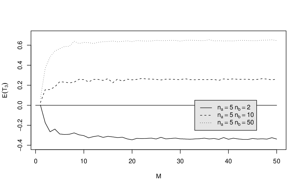
where and independently, and the cluster sizes are generated via . The dependency of cluster size on the realizations of induces the informative cluster size property. We wish to estimate the population mean which is zero in this case. and are naturally unbiased, that is,
The regular sample mean
where , is generally not unbiased and not even consistent for . In fact, there is no corresponding functional . The expected value of depends not only on and , but also on (see Figure 1).
The variances of the two unbiased estimators and are, of course, quite different:
and we conclude that
is the preferred estimate for the population quantity .
Remark 2.
If it cannot be assumed that are exchangeable, a location center can still be defined as an expected value of a randomly chosen observation in a random cluster, which still serves as a descriptive statistic of the distribution. This functional is then defined in the sample space of
where is a pseudo random variable uniformly distributed in . Also and are conditionally independent conditioned on . Let be the resulting probability measure. Then the location functional is . It is then straightforward to see that
If are exchangeable, then is naturally equal to . The resulting estimate is again
This can be generalized into cases where is not necessarily uniformly distributed.
Remark 3.
If the cluster size is noninformative, exchangeable, and we wish to estimate , all the weighted means
are unbiased. Optimal weights can be found in some simple settings. Recall that, for informative cluster size, weights proportional to in the th cluster guarantee unbiasedness. It may be possible to find other classes of weights that would also result in estimates having this property.
In a similar way, there are several possible functionals for the variance of . Again,
is biased,
is appropriate under exchangeability but loses information, and
is the most natural modification of the sample variance in this setting. It is only asymptotically unbiased. Unlike in the standard setting, a general correction term to correct for the bias in finite samples cannot be given. The variance functional corresponding to is naturally
3.2 Other distribution functionals
Let denote the marginal distribution of a randomly chosen in a random cluster. The cumulative distribution function and the corresponding quantiles still serve as useful summary measures of the marginal distribution even when exchangeability assumption is violated (Remark 2). A natural functional for is
The corresponding quantile functional satisfies
The properly estimated cumulative distribution function yield corresponding estimates of quantiles as well. The conventional estimate is biased for these purposes and there is no corresponding functional.
Even though the correct functional form may appear obvious, we stress that this simple functional structure must be maintained in all levels when the functional nests other functionals within it. This need for caution can be demonstrated by investigating the correct functional of the -trimmed mean
where the and are the corresponding quantiles. Now the quantiles themselves are functionals which should be based on the correctly defined cumulative distribution functionals.
Another example is the sample correlation, where the correct functional form employs three redefined functionals, as shown by Example 5.
Example 5 (Sample correlation coefficient).
Suppose that we observe a sample of i.i.d. clusters with bivariate observations
where with and . Thus, and are uncorrelated but the cluster size is informative in the following way. Assume that large cluster sizes appear only when both components are large,
where and . Consider the biases of different sample statistics for at . First,
where
Deviation from zero indicates linear dependency and thus, it is clearly not a good estimate of the marginal covariance functional of interest. The weighted covariance functional
is still off the target because of the biased location estimate, and the correct covariance functional,
where the estimate of the mean vector is
The appropriate covariance functional is
To estimate the unknown correlation coefficient , the correct covariance functional should be standardized using the square root of the product of appropriately defined marginal variance functionals.
Example 5 shows that incorrect functional forms can indicate dependency when it is actually an artefact caused by informative cluster size. The opposite, incorrect functionals suggesting no dependency in presence of real correlation, could also happen in a setting where the cluster sizes are related to the outcomes in a specific way.
3.3 Sign and rank based functionals
Much of the literature on informative cluster size has been on nonparametric methods. It thus makes sense to define the basic sign and rank concepts and related quantities in the same functional spirit.
Suppose that the interest lies in the median of the distribution of rather than its expected value. Alternative location functionals for this marginal median are then and which satisfy
respectively. Then is the sample median of observations and is the weighted median of all observations with weights proportional to in the th cluster. In the sign test one confronts the hypotheses
A modified sign test statistic related to is
which is a special case of weighted sign tests considered by Larocque et al. (2007), but in the case of noninformative cluster size, with weights chosen as . Again, standard asymptotics show that the standardized and quadratic form of the test statistic has a limiting chi-square distribution with one degree of freedom under the null hypothesis.
A signed-rank test for informative cluster size problems was considered by Datta and Satten (2008). Their test is based on the within-cluster resampling approach proposed by Hoffman et al. (2001), which cleverly avoids the modeling of the covariance structure. The concepts of rank and signed-rank can be defined in an informative cluster size setting in a functional manner. The estimate for the cumulative distribution functional is
An apparent modification of the rank of is, accordingly, . For the signed-rank concept we first need
and then the signed-rank of is . The signed-rank test statistic for testing whether the symmetry center of the distribution of is zero is then
This test has been proposed in Datta and Satten (2008), where also the limiting distribution is found via the resampling strategy.
To define the Hodges-Lehmann location functional for the distribution of we need, as in the i.i.d. case, two independent copies of the distribution of , say, and . Alternative location functionals and satisfy
respectively. Note then that is the Hodges-Lehmann estimate calculated from observations and is the weighted Hodges-Lehmann estimate based on all observations. The signed-rank test given above is related to the latter functional.
3.4 Regression functionals
In the linear regression case the cluster variables are . On each cluster, we observe cluster sizes , a matrix consisting of multivariate outcomes and a matrix of covariates . Assume that
are exchangeable and that, for the correct , . Possible regression coefficient functionals in this case are and satisfying
Then is the least squares estimate based on and is a weighted least squares estimate using all the observations in the appropriate way. Again, in the case of informative sample size, there is no functional corresponding to the naive estimate satisfying
It is useful to note that from the estimating equation
we get by straightforward calculation that
and that
where with , . The first part of the right hand side converges in probability to its expected value, and the second part clearly has a limiting normal distribution. Thus, the statistical inference on the regression coefficients can be based on a normal distribution with mean zero and a covariance matrix, which can be estimated by the sandwiching form , where
For cases where are not exchangeable, we can define in the sample space of
by
Functional then is a measure of “average regression”.
In standard cluster specific random effects models, if the cluster size distribution only depend on the random effect but not on the covariates, then a simple calculation shows that the corresponding components of the estimators without the weight also converge to the correct regression parameters. In other words, in such cases, the classical analyses will also work for such parameters but the estimates of the other parameters including the intercept terms will continue to be biased. Benhin et al. (2005), Gueorguieva (2005), Wang et al. (2011) and Neuhaus and McCulloch (2011), e.g., consider these types of results.
3.5 Regression M functionals
In the univariate case, simultaneous (naive) M functionals and for linear regression are given by equations
where now
Recall that, in maximum likelihood estimation,
and Huber’s estimate, for example, is given by
with tuning parameters . Alternative functionals for clustered data with informative cluster size are given by
Iteration steps to compute the estimates and are:
- 1.
first update the residuals
- 2.
next the weights
- 3.
and finally obtain new values of and as
The covariance matrix estimate of can be approximated by the sandwich estimate where now
4 Test construction
Suppose that the null hypothesis of interest implies that (or can be formulated as)
where corresponds to the probability measure overlying the distribution of , plus the covariates in the regression case, if they are assumed to be random, too. An appropriate test statistic for this testing problem based on i.i.d. observations (plus covariates in case of regression) is simply given by
As for example, if we are interested in testing , then the null hypothesis implies that also with . While is a valid test statistic, it is objectionable: (i) this may be inefficient since a large part of the data will be ignored depending on which observations are chosen by the particular realization of the random indices and (ii) the artificial randomization itself may be unsatisfactory for practical application and may lead to additional variability. Therefore, an appropriate strategy will be to take a further expectation of this test statistic with respect to conditional distribution of the indices given the original clustered data leading to the test statistic
Depending on the problem, this can sometimes be analytically calculated exactly or approximately (up to terms that are asymptotically ignorable, as ) through a linear approximation of (Datta and Satten, 2005; Datta and Satten, 2008). In the one sample problem of testing location symmetry, Datta and Satten (2008) adopted the signed-rank statistic for clustered data by selecting to be the regular signed-rank statistic for i.i.d. data. It turns out that the resulting is algebraically equivalent to the signed-clustered rank test statistic we obtained in Section 3 from an intuitive consideration via statistical functional.
The test statistic can always be estimated using a Monte-Carlo technique that is in the same spirit of the original within-cluster resampling proposal by Hoffman et al. (2001) for the estimation problem:
where a large number sets of realizations of the random indices are drawn.
An estimate of the sampling variance of this test statistic can be computed in one of three possible ways:
- (i)
by analytical calculation involving linearization techniques such as projections;
- (ii)
by the Monte-Carlo variance formula
with the assumption that one has a variance formula for the statistic ; or
- (iii)
by bootstrap resampling of the entire cluster of observations and by empirical variance of the test values of the test statistics calculated with the resampled data.
Example 6 (A modified t-test).
An immediate modification of the -test in conjunction with informative cluster size is as follows. The goal is to confront the null hypothesis with the alternative , where is uniformly distributed. Alternatively, the null can be formulated as , which gives the test statistic . As tends to infinity, the limiting distribution of the modified one-sample -statistic is
where
is a consistent estimate of the limiting variance of , because are i.i.d. with expectation zero under the null.
5 A data example on patients with incomplete spinal cord injuries
This data set is based on an observational cohort of patients at the NeuroRecovery Network (NRN). Patients eligible for NRN have incomplete spinal cord injuries (SCI) with lesion at level T10 or above and are not participating in inpatient rehabilitation programs (Harkema et al., 2012). Patients are discharged from the NRN for non-compliance with treatment, patient election, or if a plateau in the recovery of function is achieved. This last discharge criterion is of particular interest to the present analysis and is the reason for the potential informativeness of the cluster size. More severely impaired patients tended to have more “room for improvement” in function and hence remained enrolled in the NRN for longer periods of time, contributing more observations than those that enrolled with higher pre-existing function. This phenomenon has been previously demonstrated for NRN patients (Figure 2).
The outcome measures per longitudinal evaluation are as follows: The Ten Meter Walk Test is commonly used as a measure of walking capacity in SCI patients. In each test, a patient is instructed to walk as fast (10MW) as possible without assistance from the therapist conducting the assessment. The reliability and validity of this test in measuring walking function has previously been demonstrated (van Hedel et al., 2005).
The sample mean of the ten meter walking speed (meters/second) is . The weighted mean (weights inversely proportional to cluster size) is . This indicates that the marginal mean is underestimated without the proper weighting; in fact, does not estimate any population functional and it is therefore not a proper estimate. The sample statistic does not estimate the same quantity as , either, because the assumption of exchangeability is not reasonable due to improvement in patient conditions over time (Figure 2).
We investigate for further illustration purposes the behavior of four estimates of in the linear model of the form
for studying the effects of gender (1 if male; 0 if female) and four races (indicators race, race3) on the results of the Ten Meter Walk Test (the Ten Meter Walk speed). There are patients with at least one test result and test results with non-missing values on the covariates. The four estimates of regression coefficients and their standard errors are obtained as follows.
- 1.
Within-cluster resampling (WCR) with 1000 resamples. The model is fitted using ordinary least squares on each resample. Variances and standard errors of the regression coefficients are estimated by the Monte-Carlo variance formula given in section 4.
- 2.
Ordinary least squares (OLS) fitted on the full data completely ignoring the clustering.
- 3.
Inverse cluster size weighted least squares (ICSWLS) with weights inversely proportional to cluster size, and fitted on the full data. Standard errors are derived from the sandwich estimator of the covariance matrix given in section 3.
- 4.
Linear mixed model (MM) with an additional patient random effect. Parameter estimates and their standard errors are derived via restricted maximum likelihood estimation using inverse of the covariance matrix as the weight matrix.
- 5.
Inverse cluster size weighted Huber’s regression (ICWHR) estimate with and accompanied with standard errors derived from the corresponding sandwich estimator of the covariance.
| Estimate (standard error) | ||||||||||
|---|---|---|---|---|---|---|---|---|---|---|
| Parameter | WCR | OLS | ICSWLS | MM | ICWHR | |||||
| Intercept | 0.418 | (0.216) | 0.297 | (0.104) | 0.420 | (0.203) | 0.415 | (0.211) | 0.385 | (0.169) |
| gender | 0.139 | (0.064) | 0.107 | (0.029) | 0.138 | (0.059) | 0.137 | (0.064) | 0.094 | (0.047) |
| race1 | 0.086 | (0.220) | 0.172 | (0.107) | 0.086 | (0.218) | 0.088 | (0.214) | 0.031 | (0.176) |
| race2 | 0.042 | (0.244) | 0.258 | (0.119) | 0.040 | (0.229) | 0.053 | (0.238) | 0.032 | (0.216) |
| race3 | -0.060 | (0.211) | 0.038 | (0.102) | -0.061 | (0.202) | -0.056 | (0.207) | -0.063 | (0.167) |
WCR and ICSWLS approaches result into nearly identical parameter estimates and they are both known to be unbiased. Differences are attributable to randomness arising from resampling. Their standard errors are similar throughout. OLS estimates are biased, and severely so. The regression coefficient for race3, even has a different sign. Furthermore, the standard errors of the estimates are artificial and much too small as they do not account for the clustering. The parameter estimates from the linear mixed model often fall between ICSWLS and OLS estimates and are not far off, either. It has been noted that under specific conditions, a linear mixed model can result into consistent estimates of the slope parameters (Neuhaus and McCulloch, 2011); a finding that is supported by these analyses. This, however, is not the case even in a random intercepts model if the covariate is related to the cluster sizes (Wang et al., 2011; Lorenz et al., 2011). In our setting the explanatory variables are not closely related to the cluster sizes and this is a potential reason for the good performance of the linear mixed model here. Among these methods, our preference would be the ICSWLS leading to unbiased estimates without computational burden due to resampling of data. Inverse cluster size weighted Huber’s estimate provides a robust alternative to these methods and performs extremely well for this particular data set with similar estimates of regression coefficients and smaller standard errors throughout.
6 Concluding remarks
This paper gives an account on appropriate models, summary statistics and generalizing statistical classical, nonparametric and robust procedures on clustered data with possibly informative cluster size. We have demonstrated how subtle the problem is, and hope to have convinced the reader of a general method of dealing with it by appropriate functionals, leading to weighted sample statistics. In fact, it seems to us that the whole classical statistical theory, and the theory of robust statistical procedures with the concepts such as the breakdown point and influence function can be reformulated along these lines for informative cluster size problems.
It is clear that not all clustered data suffer from informative cluster size. Nevertheless, it seems like a good idea to investigate the distribution of the responses as function of the cluster size by means of graphical summaries or similar, to make sure this is not the case. Note, however, that the proposed modified properties are valid also if the cluster size is not informative, at the possible cost of losing some efficiency relative to optimally weighted procedures.
Acknowledgements
This research was supported by the Academy of Finland and by NIH grants 1R03DE020839-01A1, 5R03DE020839-02 and 1R03DE022538-01. The authors are grateful for the use of data from the NeuroRecovery Network, and thank the directors of centers participating in the NRN: Steve Ahr (Frazier Rehab Institute, Louisville, KY), Steve Williams, MD (Boston Medical Center, Boston, MA), Daniel Graves, PhD (Memorial Hermann/The Institute of Rehabilitation and Research, Houston, TX), Keith Tansey, MD, PhD (Shepherd Center, Atlanta, GA), Gail Forrest, PhD (Kessler Medical Rehabilitation Research and Education Corporation, West Orange, NJ), D. Michele Basso PT, EdD (The Ohio State University Medical Center, Columbus, OH) and Mary Schmidt Read, PT, DPT, MS (Magee Rehabilitation, Philadelphia, PA).
References
- Benhin et al. (2005) E. Benhin, J. N. K. Rao, and A. J. Scott. Mean estimating equation approach to analysing cluster-correlated data with nonignorable cluster sizes. Biometrika, 92:435–450, 2005.
- Bickel and Lehmann (1975a) P. J. Bickel and E. L. Lehmann. Descriptive statistics for nonparametric models. I. Introduction. The Annals of Statistics, 3:1038–1044, 1975a.
- Bickel and Lehmann (1975b) P. J. Bickel and E. L. Lehmann. Descriptive statistics for nonparametric models. II. Location. The Annals of Statistics, 3:1045–1069, 1975b.
- Billingsley (1995) P. Billingsley. Probability and Measure. John Wiley & Sons, New York, USA, third edition, 1995.
- Chiang and Lee (2008) C.-T. Chiang and K.-Y. Lee. Efficient estimation methods for informative cluster size data. Statistica Sinica, 18:121–133, 2008.
- Datta and Satten (2005) S. Datta and G. A. Satten. Rank-sum tests for clustered data. Journal of the American Statistical Association, 100:908–915, 2005.
- Datta and Satten (2008) S. Datta and G. A. Satten. A signed-rank test for clustered data. Biometrics, 64:501–507, 2008.
- Dunson et al. (2003) D. B. Dunson, Z. Chen, and J. Harry. A Bayesian approach for joint modeling of cluster size and subunit-specific outcomes. Biometrics, 59:521–530, 2003.
- Gueorguieva (2005) R. V. Gueorguieva. Comments about joint modeling of cluster size and binary and continuous subunit-specific outcomes. Biometrics, 61:862–867, 2005.
- Harkema et al. (2012) S. J. Harkema, M. Schmidt-Read, A. Behrman, A. Bratta, S. A. Sisto, and V. R. Edgerton. Establishing the neurorecovery network: multi-site rehabilitation centers that provide activity based therapies and assessments for neurologic disorders. Archives of Physical Medicine and Rehabilitation, 93:1498–1507, 2012.
- Hoffman et al. (2001) E. B. Hoffman, P. K. Sen, and C. R. Weinberg. Within-cluster resampling. Biometrika, 88:1121–1134, 2001.
- Huang and Chen (2003) Y. Huang and Y. Q. Chen. Marginal regression of gaps between recurrent events. Lifetime Data Anal, 9(3):293–303, Sep 2003.
- Larocque et al. (2007) D. Larocque, J. Nevalainen, and H. Oja. A weighted multivariate sign test for cluster correlated data. Biometrika, 94:267–283, 2007.
- Lorenz et al. (2011) D. J. Lorenz, S. Datta, and S. J. Harkema. Marginal association measures for clustered data. Statistics in Medicine, 30(27):3181–3191, Nov 2011. doi: 10.1002/sim.4368. URL http://dx.doi.org/10.1002/sim.4368.
- Neuhaus and McCulloch (2011) J. M. Neuhaus and C. E. McCulloch. Estimation of covariate effects in generalized linear mixed models with informative cluster sizes. Biometrika, 98:147–162, 2011.
- Panageas et al. (2007) K. S. Panageas, D. Schrag, L. A. Russell, E. S. Venkatraman, and C. B. Begg. Properties of analysis methods that account for clustering in volume-outcome studies when the primary predictor is cluster size. Statistics in Medicine, 26:2017–2035, 2007.
- van Hedel et al. (2005) H. van Hedel, M. Wirz, and V. Dietz. Assessing walking ability in subjects with spinal cord injury: validity and reliability of 3 walking tests. Archives of Physical Medicine and Rehabilitation, 86:190–196, 2005.
- Wang et al. (2011) M. Wang, M. K. Kong, and S. Datta. Inference for marginal linear models for clustered longitudinal data with potentially informative cluster sizes. Statistical Methods in Medical Research, 20:347–367, 2011. doi: doi: 10.1177/0962280209347043.
- Williamson et al. (2003) J. M. Williamson, S. Datta, and G. A. Satten. Marginal analyses of clustered data when cluster size is informative. Biometrics, 59:36–42, 2003.
- Williamson et al. (2007) J. M. Williamson, H.-Y. Kim, and L. Warner. Weighting condom use data to account for nonignorable cluster size. Annals of Epidemiology, 17:603–607, 2007.
- Williamson et al. (2008) J. M. Williamson, H.-Y. Kim, A. Manatunga, and D. G. Addiss. Modeling survival data with informative cluster size. Statistics in Medicine, 27:543–555, 2008.