Slow and Stale Gradients Can Win the Race: Error-Runtime Trade-offs in Distributed SGD

Single Node SGD: Analysis of gradient descent dates back to classical works [3] in the optimization community. The problem of interest is the minimization of empirical risk of the form:

Here, $\xi_{n}$ denotes the $n-$th data point and its label where $n=1,2,\dots,N$, and $f(\mathbf{w},\xi_{n})$ denotes the composite loss function. Gradient descent is a way to iteratively minimize this objective function by updating the parameter $\mathbf{w}$ in the opposite direction of the gradient of $F(\mathbf{w})$ at every iteration, as given by:

The computation of $\sum_{n=1}^{N}\nabla f(\mathbf{w}_{j},\xi_{n})$ over the entire dataset is expensive. Thus, stochastic gradient descent [4] with mini-batching is generally used in practice, where the gradient is evaluated over small, randomly chosen subsets of the data. Smaller mini-batches result in higher variance of the gradients, which affects convergence and error floor [5, 6, 7]. Algorithms such as AdaGrad [8] and Adam [9] gradually reduce learning rate to achieve a lower error floor. Another class of algorithms includes stochastic variation reduction techniques that include SVRG [10], SAGA [11] and their variants listed out in [12]. For a detailed survey of different SGD variants, refer to [13].

Synchronous SGD and Stragglers: To process large datasets, SGD is parallelized across multiple learners with a central PS. Each learner processes one mini-batch, and the PS aggregates all the gradients. The convergence of synchronous SGD is same as mini-batch SGD, with a $P$-fold larger mini-batch, where $P$ is the number of learners. However, the time per iteration grows with the number of learners, because some straggling learners that slow down randomly [2]. Thus, it is important to juxtapose the error reduction per iteration with the runtime per iteration to understand the true convergence speed of distributed SGD.

To deal with stragglers and speed up machine learning, system designers have proposed several straggler mitigation techniques such as [14] that try to detect and avoid stragglers. An alternate direction of work is to use redundancy techniques, e.g., replication or erasure codes, as proposed in [15, 16, 17, 18, 19, 20, 21, 22, 23, 24, 25, 26, 27, 28, 29, 30, 31, 32, 33, 34, 35] to deal with the stragglers, as also discussed in Remark 1.

Asynchronous SGD and Staleness: A complementary approach to deal with the issue of straggling is to use asynchronous SGD. In asynchronous SGD, any learner can evaluate the gradient and update the central PS without waiting for the other learners. Asynchronous variants of existing SGD algorithms have also been proposed and implemented in systems [1, 36, 37, 38, 39].

In general, analyzing the convergence of asynchronous SGD with the number of iterations is difficult in itself because of the randomness of gradient staleness. There are only a few pioneering works such as [40, 41, 42, 43, 44, 45, 46, 47, 48, 49, 50, 51, 52] in this direction. In [40], a fully decentralized analysis was proposed that considers no central PS. In [43], a new asynchronous algorithm called Hogwild was proposed and analyzed under bounded gradient and bounded delay assumptions. This direction of research has been followed upon by several interesting works such as [41] which proposed novel theoretical analysis under bounded delay assumption for other asynchronous SGD variants. In [48, 49, 50, 51], the framework of ARock was proposed for parallel co-ordinate descent and analyzed using Lyapunov functions, relaxing several existing assumptions such as bounded delay assumption and the independence of the delays and the index of the blocks being updated. In algorithms such as Hogwild, ARock etc. every learner only updates a part of the central parameter vector $\mathbf{w}$ at every iteration and are thus essentially different in spirit from conventional asynchronous SGD settings [41, 44] where every learner updates the entire $\bm{\mathbf{w}}$. In an alternate direction of work [45], asynchrony is modelled as a perturbation.

Existing machine learning algorithms mostly try to optimize the trade-off of error with the number of iterations, epochs or “work complexity” [7]. Time to complete a task has traditionally been calculated in terms of work complexity measures [53], where the time taken to complete a task is a deterministic function of the size of the task (number of operations). However, due to straggling and synchronization bottle-necks in the system, the same task can often take different time to compute across different learners or iterations. We bring statistical perspective to the traditional work complexity analysis that incorporates the randomness introduced due to straggling. In this paper, we provide a systematic approach to analyze the expected error with runtime for both synchronous and asynchronous SGD, and some variants like $K$-sync, $K$-batch-sync, $K$-async and $K$-batch-async SGD by modelling the runtimes at each learner as i.i.d. random variables with a general distribution.

We also propose a new error convergence analysis for Async and $K$-async SGD that holds for strongly convex objectives and can also be extended to non-convex formulations. In this analysis we relax the bounded delay assumption in [41] and the bounded gradient assumption in [43]. We also remove the assumption of exponential computation time and the staleness process being independent of the parameter values [42] as we will elaborate in Section 3.2. Interestingly, our analysis also brings out the regimes where asynchrony can be better or worse than synchrony in terms of speed of convergence. Further, we propose a new learning rate schedule to compensate for staleness, and stabilize asynchronous SGD that is related but different from momentum tuning in [42, 54] as we clarify in Remark 2.

The rest of the paper is organized as follows. Section 2 describes our problem formulation introducing the system model and assumptions. Section 3 provides the main results of the paper – analytical characterization of expected runtime and new convergence analysis for Async and $K$-async SGD and the proposed learning rate schedule to compensate for staleness. The analysis of expected runtime is elaborated further in Section 4. Proofs and detailed discussions are presented in the Appendix.

We assume that there is a central parameter server (PS) with $P$ parallel learners as shown in Figure 2. The learners fetch the current parameter vector $\mathbf{w}_{j}$ from the PS as and when instructed in the algorithm. Then they compute gradients using one mini-batch and push their gradients back to the PS as and when instructed in the algorithm. At each iteration, the PS aggregates the gradients computed by the learners and updates the parameter $\mathbf{w}$. Based on how these gradients are fetched and aggregated, we have different variants of synchronous or asynchronous SGD.

The time taken by a learner to compute gradient of one mini-batch is denoted by random variable $X_{i}$ for $i=1,2,\dots,P$. We assume that the $X_{i}$s are i.i.d. across mini-batches and learners.

There are two metrics of interest: Expected Runtime and Error.

Our aim is to determine the trade-off between the expected error (measures the accuracy of the algorithm) and the expected runtime after a total of $J$ iterations for the different SGD variants.

We now describe the SGD variants considered in this paper. Please refer to Figure 3 and Figure 4 for a pictorial illustration.

$K$-sync SGD: This is a generalized form of synchronous SGD, also suggested in [36, 55] to offer some resilience to straggling as the PS does not wait for all the learners to finish. The PS only waits for the first $K$ out of $P$ learners to push their gradients. Once it receives $K$ gradients, it updates $\mathbf{w}_{j}$ and cancels the remaining learners. The updated parameter vector $\mathbf{w}_{j+1}$ is sent to all $P$ learners for the next iteration. The update rule is given by:

Here $l=1,2,\ldots,K$ denotes the index of the $K$ learners that finish first, $\xi_{l,j}$ denotes the mini-batch of $m$ samples used by the $l$-th learner at the $j$-th iteration and $g(\mathbf{w}_{j},\xi_{l,j})=\frac{1}{m}\sum_{\xi\in\xi_{l,j}}\nabla f(\mathbf{w}_{j},\xi)$ denotes the average gradient of the loss function evaluated over the mini-batch $\xi_{l,j}$ of size $m$. For $K=P$, the algorithm is exactly equivalent to a fully synchronous SGD with $P$ learners.

$K$-batch-sync: In $K$-batch-sync, all the $P$ learners start computing gradients with the same $\mathbf{w}_{j}$. Whenever any learner finishes, it pushes its update to the PS and evaluates the gradient on the next mini-batch at the same $\mathbf{w}_{j}$. The PS updates using the first $K$ mini-batches that finish and cancels the remaining learners. Theoretically, the update rule is still the same as 2 but here $l$ now denotes the index of the mini-batch (out of the $K$ mini-batches that finished first) instead of the learner. However $K$-batch-sync will offer advantages over $K$-sync in runtime per iteration as no learner is idle.

$K$-async SGD: This is a generalized version of asynchronous SGD, also suggested in [36]. In $K$-async SGD, all the $P$ learners compute their respective gradients on a single mini-batch. The PS waits for the first $K$ out of $P$ that finish first, but it does not cancel the remaining learners. As a result, for every update the gradients returned by each learner might be computed at a stale or older value of the parameter $\mathbf{w}$. The update rule is thus given by:

Here $l=1,2,\ldots,K$ denotes the index of the $K$ learners that contribute to the update at the corresponding iteration, $\xi_{l,j}$ is one mini-batch of $m$ samples used by the $l$-th learner at the $j$-th iteration and $\tau(l,j)$ denotes the iteration index when the $l$-th learner last read from the central PS where $\tau(l,j)\leq j$. Also, $g(\mathbf{w}_{\tau(l,j)},\xi_{l,j})=\frac{1}{m}\sum_{\xi\in\xi_{l,j}}\nabla f(\mathbf{w}_{\tau(l,j)},\xi_{l,j})$ is the average gradient of the loss function evaluated over the mini-batch $\xi_{l,j}$ based on the stale value of the parameter $\mathbf{w}_{\tau(l,j)}$. For $K=1$, the algorithm is exactly equivalent to fully asynchronous SGD, and the update rule can be simplified as:

Here $\xi_{j}$ denotes the set of samples used by the learner that updates at the $j$-th iteration such that $|\xi_{j}|=m$ and $\tau(l,j)$ denotes the iteration index when that particular learner last read from the central PS. Note that $\tau(j)\leq j$.

$K$-batch-async: Observe in Figure 4 that $K$-async also suffers from some learners being idle while others are still working on their gradients until any $K$ finish. In $K$-batch-async (proposed in [41]), the PS waits for $K$ mini-batches before updating itself but irrespective of which learner they come from. So wherever any learner finishes, it pushes its gradient to the PS, fetches current parameter at PS and starts computing gradient on the next mini-batch based on the current value of the PS. Surprisingly, the update rule is again similar to 3 theoretically except that now $l$ denotes the indices of the $K$ mini-batches that finish first instead of the learners and $\mathbf{w}_{\tau(l,j)}$ denotes the version of the parameter when the learner computing the $l-$th mini-batch last read from the PS. While the error convergence of $K$-batch-async is similar to $K$-async, it reduces the runtime per iteration as no learner is idle.

Closely following [7], we also make the following assumptions:

1. 1.

   $F(\mathbf{w})$ is an $L-$ smooth function. Thus,

   $$||\nabla F(\mathbf{w}_{1})-\nabla F(\mathbf{w}_{2})||_{2}\leq L||\mathbf{w}_{1}-\mathbf{w}_{2}||_{2}.$$

   (5)

2. 2.

   $F(\mathbf{w})$ is strongly convex with parameter $c$. Thus,

   $$2c(F(\mathbf{w})-F^{*})\leq||\nabla F(\mathbf{w})||_{2}^{2}\ \ \forall\ \mathbf{w}.$$

   (6)

   Refer to Appendix A for discussion on strong convexity. Our results also extend to non-convex objectives, as discussed in Section 3.

3. 3.

   The stochastic gradient is an unbiased estimate of the true gradient:

   $$\mathbb{E}_{\xi_{j}|\mathbf{w}_{k}}\left[{g(\mathbf{w}_{k},\xi_{j})}\right]=\nabla F(\mathbf{w}_{k})\ \ \forall\ k\leq j.$$

   (7)

   Observe that this is slightly different from the common assumption that says $\mathbb{E}_{\xi_{j}}\left[{g(\mathbf{w},\xi_{j})}\right]=\nabla F(\mathbf{w})$ for all $\mathbf{w}$. Observe that all $\mathbf{w}_{j}$ for $j>k$ is actually not independent of the data $\xi_{j}$. We thus make the assumption more rigorous by conditioning on $\mathbf{w}_{k}$ for $k\leq j$. Our requirement $k\leq j$ means that $\mathbf{w}_{k}$ is the value of the parameter at the PS before the data $\xi_{j}$ was accessed and can thus be assumed to be independent of the data $\xi_{j}$.

4. 4.

   Similar to the previous assumption, we also assume that the variance of the stochastic update given $\mathbf{w}_{k}$ at iteration $k$ before the data point was accessed is also bounded as follows:

   $\displaystyle\mathbb{E}_{\xi_{j}|\mathbf{w}_{k}}\left[{||g(\mathbf{w}_{k},\xi_{j})-\nabla F(\mathbf{w}_{k})||_{2}^{2}}\right]\leq\frac{\sigma^{2}}{m}+\frac{M_{G}}{m}||\nabla F(\mathbf{w}_{k})||_{2}^{2}\ \forall\ k\leq j.$

   (8)

In the following Table 1, we provide a list of the notations used in this paper for referencing.

We compare the theoretical wall clock runtime of the different SGD variants to illustrate the speed-up offered by different asynchronous and batch variants. A detailed discussion is provided in Section 4.

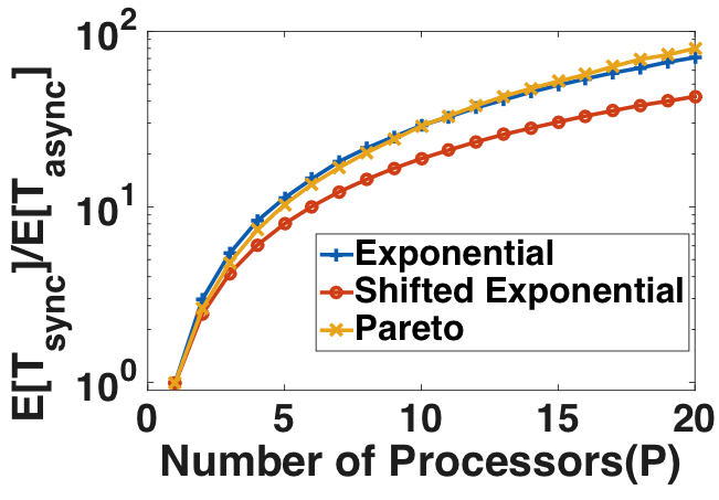
This result analytically characterizes the speed-up offered by asynchronous SGD for any general distribution on the wall clock time of each learner. To prove this result, we use ideas from renewal theory, as we discuss in Section 4. In the following corollary, we highlight this speed-up for the special case of exponential computation time.

Thus, the speed-up scales with $P$ and can diverge to infinity for large $P$. We illustrate the speed-up for different distributions in Figure 5. It might be noted that a similar speed-up as Corollary 1 has also been obtained in a recent work [49] under exponential assumptions.

The next result illustrates the advantages offered by $K$-batch-sync and async over their corresponding counterparts $K$-sync and $K$-async respectively.

To prove this, we derive an exact expression (see Lemma 5 in Section 4) for the expected runtime of $K$-batch-async SGD, for any given i.i.d. distribution of $X_{i}$s, not necessarily exponential. The expected runtime per iteration is obtained as $\frac{K\mathbb{E}\left[{X}\right]}{P}$, using ideas from renewal theory. The full proof of Theorem 2 is also provided in Section 4.

Theorem 2 shows that as $\frac{K}{P}$ increases, the speed-up using $K$-batch-async increases and can be upto $\log{P}$ times higher. For non-exponential distributions, we simulate the behaviour of expected runtime in Figure 6 for $K$-sync, $K$-async and $K$-batch-async respectively for Pareto and Shifted Exponential.

Theorem 3 below gives a convergence analysis of $K$-async SGD for fixed $\eta$, relaxing the following assumptions in existing literature.

• •

  In several prior works such as [42, 19, 21, 49], it is often assumed, for the ease of analysis, that runtimes are exponentially distributed. In this paper, we extend our analysis for any general service time $X_{i}$.

• •

  In [42], it is also assumed that the staleness process is independent of $\mathbf{w}$. While this assumption simplifies the analysis greatly, it is not true in practice. For instance, for a two learner case, the parameter $\mathbf{w}_{2}$ after $2$ iterations depends on whether the update from $\mathbf{w}_{1}$ to $\mathbf{w}_{2}$ was based on a stale gradient at $\mathbf{w}_{0}$ or the current gradient at $\mathbf{w}_{1}$, depending on which learner finished first. In this work, we remove this independence assumption.

• •

  Instead of the bounded delay assumption in [41], we use a general staleness bound

  $$\mathbb{E}\left[{||\nabla F(\mathbf{w}_{j})-\nabla F(\mathbf{w}_{\tau(l,j)})||_{2}^{2}}\right]\leq\gamma\mathbb{E}\left[{||\nabla F(\mathbf{w}_{j})||_{2}^{2}}\right]$$

  which allows for large, but rare delays.

• •

  In [43], the norm of the gradient is assumed to be bounded. However, if we assume that $||\nabla F(\mathbf{w})||_{2}^{2}\leq M$ for some constant $M$, then using 6 we obtain $||\mathbf{w}-\mathbf{w}^{*}||_{2}^{2}\leq\frac{2}{c}(F(\mathbf{w})-F^{*})\leq\frac{M}{c^{2}}$ implying that $\mathbf{w}$ itself is bounded which is a very strong and restrictive assumption, that we relax in this result.

Here, $\gamma$ is a measure of staleness of the gradients returned by learners; smaller $\gamma$ indicates less staleness.

The full proof is provided in Appendix C. We first prove the result for $K=1$ in Section C.1 for ease of understanding, and then provide the more general proof for any $K$ in Section C.2. We use Lemma 1 below to prove Theorem 3.

For the exponential distribution, $p_{0}$ is equal to $\frac{1}{P}$ as we discuss in Lemma 2. For non-exponential distributions, it is a constant in $[0,1]$. For some special classes of distributions like new-longer-than-used (new-shorter-than-used) as defined in Definition 3, we can formally show that $p_{0}$ lies in $[0,\frac{1}{P}]$ ($[\frac{1}{P},1]$) respectively. The following Lemma 2 below provides bounds on $p_{0}$.

The proof is provided in Section C.1.1.

For $K$-batch-async, the update rule is same as $K$-async except that the index $l$ denotes the index of the mini-batch. Thus, the error analysis will be exactly similar. Our analysis can also be extended to non-convex $F(\mathbf{w})$ as we show in Section C.2.1.

Now let us compare with $K$-sync SGD. We observe that the analysis of $K$-sync SGD is same as serial SGD with mini-batch size $Km$. Thus,

Can stale gradients win the race? For the same $\eta$, observe that the error given by Theorem 3 decays at the rate $(1-\eta c(1-\gamma+\frac{p_{0}}{2}))$ for $K$-async or $K$-batch-async SGD while for $K$-sync, the decay rate with number of iterations is $(1-\eta c)$. Thus, depending on the values of $\gamma$ and $p_{0}$, the decay rate of $K$-async or $K$-batch-async SGD can be faster or slower than $K$-sync SGD. The decay rate of $K$-async or $K$-batch-async SGD is faster if $\frac{p_{0}}{2}>\gamma$. As an example, one might consider an exponential or new-shorter-than-used service time where $p_{0}\geq\frac{1}{P}$ and $\gamma$ can be made smaller by increasing $K$. It might be noted that asynchronous SGD can still be faster than synchronous SGD with respect to wall clock time even if its decay rate with respect to number of iterations is lower as every iteration is much faster in asynchronous SGD (Roughly $P\log{P}$ times faster for exponential service times).

The maximum allowable learning rate for synchronous SGD is $\max\{\frac{1}{c},\frac{1}{2L(\frac{M_{G}}{Pm}+1)}\}$ which can be much higher than that for asynchronous SGD,i.e., $\max\{\frac{1}{c(1-\gamma+\frac{p_{0}}{2})},\frac{1}{2L(\frac{M_{G}}{m}+1)}\}$. Similarly the error-floor for synchronous is $\frac{\eta L\sigma^{2}}{2cPm}$ as compared to asynchronous whose error floor is $\frac{\eta L\sigma^{2}}{2c(1-\gamma+\frac{p_{0}}{2})m}$.

In Figure 7, we compare the theoretical trade-offs between synchronous ($K=P$ in Lemma 3) and asynchronous SGD ($K=1$ in Theorem 3). Async-SGD converges very quickly, but to a higher floor. Figure 8 shows the same comparison on the MNIST dataset, along with $K$-batch-async SGD.

The staleness of the gradient is random, and can vary across iterations. Intuitively, if the gradient is less stale, we want to weigh it more while updating the parameter $\mathbf{w}$, and if it is more stale we want to scale down its contribution to the update. With this motivation, we propose the following condition on the learning rate at different iterations.

for a constant $C$. This condition is also inspired from our error analysis in Theorem 3, because it helps remove the assumption $\mathbb{E}\left[{||\nabla F(\mathbf{w}_{j})-\nabla F(\mathbf{w}_{\tau(j)})||_{2}^{2}}\right]\leq\gamma\mathbb{E}\left[{||\nabla F(\mathbf{w}_{j})||_{2}^{2}}\right]$. Using 11, we obtain the following convergence result.

The proof is provided in Section C.3. In our analysis of Asynchronous SGD, we observe that the term $\frac{\eta}{2}\mathbb{E}\left[{||\nabla F(\mathbf{w}_{j})-\nabla F(\mathbf{w}_{\tau(j)})||_{2}^{2}}\right]$ is the most difficult to bound. For fixed learning rate, we had assumed that $\mathbb{E}\left[{||\nabla F(\mathbf{w}_{j})-\nabla F(\mathbf{w}_{\tau(j)})||_{2}^{2}}\right]$ is bounded by $\gamma||\nabla F(\mathbf{w}_{j})||_{2}^{2}$. However, if we impose the condition 11 on $\eta$, we do not require this assumption. Our proposed condition actually provides a bound for the staleness term as follows:

Thus, for a total of $J$ iterations, the expected runtime is given by $J\mathbb{E}\left[{X_{K:P}}\right]$.

The expected runtime of $K$-batch-sync SGD is not analytically tractable in general, but for $X_{i}\sim\exp(\mu)$, the runtime per iteration is distributed as $Erlang(K,P\mu)$. Refer to Section B.2 for explanation. Thus, for $K$-batch-sync SGD, the expected time per iteration is given by,

Unlike the results for the synchronous variants, this result on average runtime per iteration holds only in the limit of large number of iterations. To prove the result we use ideas from renewal theory. For a brief background on renewal theory, the reader is referred to Section B.3.

The expected runtime per iteration of $K$-async SGD is not analytically tractable for non-exponential $X_{i}$, but we obtain an upper bound on it for a class of distributions called the “new-longer-than-used” distributions, as defined below.

Most of the continuous distributions we encounter like normal, exponential, gamma, beta are new-longer-than-used. Alternately, the hyper exponential distribution is new-shorter-than-used and it satisfies $\Pr(U>u+t|U>t)\geq\Pr(U>u)$ for all $t,u\geq 0$.

The proof of this lemma is provided in Section B.4.

We provided a comparison of the expected runtimes of $K$-async and $K$-batch-async SGD variants in Theorem 2, for the special case of exponential computation times. Here, we provide the proof of Theorem 2.

The authors thank Mark Wegman, Pulkit Grover and Jianyu Wang for their suggestions and feedback.

References

- [1] Jeffrey Dean et al. Large scale distributed deep networks. In Advances in Neural Information Processing Systems, pages 1223–1231, 2012.
- [2] Jeffrey Dean and Luiz André Barroso. The tail at scale. Communications of the ACM, 56(2):74–80, 2013.
- [3] Stephen Boyd and Lieven Vandenberghe. Convex optimization. Cambridge university press, 2004.
- [4] Herbert Robbins and Sutton Monro. A stochastic approximation method. The annals of mathematical statistics, pages 400–407, 1951.
- [5] Ofer Dekel, Ran Gilad-Bachrach, Ohad Shamir, and Lin Xiao. Optimal distributed online prediction using mini-batches. Journal of Machine Learning Research, 13(1):165–202, 2012.
- [6] Mu Li, Tong Zhang, Yuqiang Chen, and Alexander J. Smola. Efficient mini-batch training for stochastic optimization. In ACM SIGKDD International Conference on Knowledge Discovery and Data Mining, pages 661–670, 2014.
- [7] Léon Bottou, Frank E. Curtis, and Jorge Nocedal. Optimization methods for large-scale machine learning. arXiv:1606.04838, 2016.
- [8] John Duchi, Elad Hazan, and Yoram Singer. Adaptive subgradient methods for online learning and stochastic optimization. Journal of Machine Learning Research, 2, July 2011.
- [9] Diederik P. Kingma and Jimmy Ba. Adam: A method for stochastic optimization. International Conference on Learning Representations (ICLR), 2015.
- [10] Rie Johnson and Tong Zhang. Accelerating stochastic gradient descent using predictive variance reduction. In Advances in Neural Information Processing Systems, pages 315–323, 2013.
- [11] Nicolas L Roux, Mark Schmidt, and Francis R Bach. A stochastic gradient method with an exponential convergence rate for finite training sets. In Advances in Neural Information Processing Systems, pages 2663–2671, 2012.
- [12] Lam M Nguyen, Jie Liu, Katya Scheinberg, and Martin Takáč. Sarah: A novel method for machine learning problems using stochastic recursive gradient. In International Conference on Machine Learning, pages 2613–2621, 2017.
- [13] Sebastian Ruder. An overview of gradient descent optimization algorithms. arXiv preprint arXiv:1609.04747, 2016.
- [14] Aaron Harlap, Henggang Cui, Wei Dai, Jinliang Wei, Gregory R. Ganger, Phillip B. Gibbons, Garth A. Gibson, and Eric P. Xing. Addressing the straggler problem for iterative convergent parallel ml. In ACM Symposium on Cloud Computing (SoCC), pages 98–111, 2016.
- [15] Gauri Joshi, Yanpei Liu, and Emina Soljanin. On the delay-storage trade-off in content download from coded distributed storage systems. IEEE Journal on Selected Areas in Communications, 32(5):989–997, 2014.
- [16] Da Wang, Gauri Joshi, and Gregory Wornell. Using straggler replication to reduce latency in large-scale parallel computing. ACM SIGMETRICS Performance Evaluation Review, 43(3):7–11, 2015.
- [17] Gauri Joshi, Emina Soljanin, and Gregory Wornell. Queues with redundancy: Latency-cost analysis. ACM SIGMETRICS Performance Evaluation Review, 43(2):54–56, 2015.
- [18] Gauri Joshi, Emina Soljanin, and Gregory Wornell. Efficient redundancy techniques for latency reduction in cloud systems. ACM Transactions on Modeling and Performance Evaluation of Computing Systems, 2(12), may 2017.
- [19] Kangwook Lee, Maximilian Lam, Ramtin Pedarsani, Dimitris Papailiopoulos, and Kannan Ramchandran. Speeding up distributed machine learning using codes. IEEE Transactions on Information Theory, 64(3):1514–1529, 2018.
- [20] Rashish Tandon, Qi Lei, Alexandros G. Dimakis, and Nikos Karampatziakis. Gradient coding: Avoiding stragglers in distributed learning. In International Conference on Machine Learning, pages 3368–3376, 2017.
- [21] Sanghamitra Dutta, Viveck Cadambe, and Pulkit Grover. Short-dot: Computing large linear transforms distributedly using coded short dot products. In Advances In Neural Information Processing Systems, pages 2100–2108, 2016.
- [22] Wael Halbawi, Navid Azizan-Ruhi, Fariborz Salehi, and Babak Hassibi. Improving distributed gradient descent using reed-solomon codes. arXiv preprint arXiv:1706.05436, 2017.
- [23] Yaoqing Yang, Pulkit Grover, and Soummya Kar. Coded distributed computing for inverse problems. In Advances in Neural Information Processing Systems, pages 709–719, 2017.
- [24] Yaoqing Yang, Pulkit Grover, and Soummya Kar. Fault-tolerant distributed logistic regression using unreliable components. In Communication, Control, and Computing (Allerton), pages 940–947. IEEE, 2016.
- [25] Qian Yu, Mohammad Maddah-Ali, and Salman Avestimehr. Polynomial codes: an optimal design for high-dimensional coded matrix multiplication. In Advances in Neural Information Processing Systems, pages 4406–4416, 2017.
- [26] Can Karakus, Yifan Sun, and Suhas Diggavi. Encoded distributed optimization. In IEEE International Symposium on Information Theory (ISIT), pages 2890–2894, 2017.
- [27] Can Karakus, Yifan Sun, Suhas Diggavi, and Wotao Yin. Straggler mitigation in distributed optimization through data encoding. In Advances in Neural Information Processing Systems, pages 5440–5448, 2017.
- [28] Zachary Charles, Dimitris Papailiopoulos, and Jordan Ellenberg. Approximate gradient coding via sparse random graphs. arXiv preprint arXiv:1711.06771, 2017.
- [29] Songze Li, Sucha Supittayapornpong, Mohammad Ali Maddah-Ali, and Salman Avestimehr. Coded terasort. In IEEE International Parallel and Distributed Processing Symposium Workshops (IPDPSW), pages 389–398, 2017.
- [30] Mohammad Fahim, Haewon Jeong, Farzin Haddadpour, Sanghamitra Dutta, Viveck Cadambe, and Pulkit Grover. On the optimal recovery threshold of coded matrix multiplication. In Communication, Control, and Computing (Allerton), pages 1264–1270. IEEE, 2017.
- [31] Min Ye and Emmanuel Abbe. Communication-computation efficient gradient coding. arXiv preprint arXiv:1802.03475, 2018.
- [32] Songze Li, Mohammad Ali Maddah-Ali, Qian Yu, and A Salman Avestimehr. A fundamental tradeoff between computation and communication in distributed computing. IEEE Transactions on Information Theory, 64(1):109–128, 2018.
- [33] Viveck Cadambe and Pulkit Grover. Codes for Distributed Computing: A Tutorial. IEEE Information Theory Society Newsletter, 67(4):3–15, December 2017.
- [34] Sanghamitra Dutta, Ziqian Bai, Haewon Jeong, Tze Meng Low, and Pulkit Grover. A Unified Coded Deep Neural Network Training Strategy based on Generalized PolyDot codes. In IEEE International Symposium on Information Theory (ISIT) - To Appear, 2018.
- [35] Ankur Mallick, Malhar Chaudhari, and Gauri Joshi. Rateless codes for near-perfect load balancing in distributed matrix-vector multiplication. arXiv preprint arXiv:1804.10331, 2018.
- [36] Suyog Gupta, Wei Zhang, and Fei Wang. Model accuracy and runtime tradeoff in distributed deep learning: A systematic study. In International Conference on Data Mining, pages 171–180, 2016.
- [37] James Cipar, Qirong Ho, Jin Kyu Kim, Seunghak Lee, Gregory R. Ganger, Garth Gibson, Kimberly Keeton, and Eric Xing. Solving the straggler problem with bounded staleness. In Workshop on Hot Topics in Operating Systems, 2013.
- [38] Henggang Cui, James Cipar, Qirong Ho, Jin Kyu Kim, Seunghak Lee, Abhimanu Kumar, Jinliang Wei, Wei Dai, Gregory R Ganger, Phillip B Gibbons, et al. Exploiting bounded staleness to speed up big data analytics. In USENIX Annual Technical Conference (ATC), pages 37–48, 2014.
- [39] Qirong Ho, James Cipar, Henggang Cui, Seunghak Lee, Jin Kyu Kim, Phillip B Gibbons, Garth A Gibson, Greg Ganger, and Eric P Xing. More effective distributed ml via a stale synchronous parallel parameter server. In Advances in Neural Information Processing Systems, pages 1223–1231, 2013.
- [40] John Tsitsiklis, Dimitri Bertsekas, and Michael Athans. Distributed asynchronous deterministic and stochastic gradient optimization algorithms. IEEE Transactions on Automatic Control, 31(9):803–812, 1986.
- [41] Xiangru Lian, Yijun Huang, Yuncheng Li, and Ji Liu. Asynchronous parallel stochastic gradient for nonconvex optimization. In Advances in Neural Information Processing Systems, pages 2737–2745, 2015.
- [42] Ioannis Mitliagkas, Ce Zhang, Stefan Hadjis, and Christopher Ré. Asynchrony begets momentum, with an application to deep learning. In Allerton Conference on Communication, Control, and Computing, pages 997–1004. IEEE, 2016.
- [43] Benjamin Recht, Christopher Re, Stephen Wright, and Feng Niu. Hogwild: A lock-free approach to parallelizing stochastic gradient descent. In Advances in Neural Information Processing Systems, pages 693–701, 2011.
- [44] Alekh Agarwal and John C Duchi. Distributed delayed stochastic optimization. In Advances in Neural Information Processing Systems, pages 873–881, 2011.
- [45] Horia Mania, Xinghao Pan, Dimitris Papailiopoulos, Benjamin Recht, Kannan Ramchandran, and Michael I Jordan. Perturbed iterate analysis for asynchronous stochastic optimization. SIAM Journal on Optimization, 27(4):2202–2229, 2017.
- [46] Sorathan Chaturapruek, John C Duchi, and Christopher Ré. Asynchronous stochastic convex optimization: the noise is in the noise and sgd don’t care. In Advances in Neural Information Processing Systems, pages 1531–1539, 2015.
- [47] Wei Zhang, Suyog Gupta, Xiangru Lian, and Ji Liu. Staleness-aware async-sgd for distributed deep learning. In International Joint Conference on Artificial Intelligence, pages 2350–2356. AAAI Press, 2016.
- [48] Zhimin Peng, Yangyang Xu, Ming Yan, and Wotao Yin. Arock: an algorithmic framework for asynchronous parallel coordinate updates. SIAM Journal on Scientific Computing, 38(5):A2851–A2879, 2016.
- [49] Robert Hannah and Wotao Yin. More iterations per second, same quality–why asynchronous algorithms may drastically outperform traditional ones. arXiv preprint arXiv:1708.05136, 2017.
- [50] Robert Hannah and Wotao Yin. On unbounded delays in asynchronous parallel fixed-point algorithms. Journal of Scientific Computing, pages 1–28, 2016.
- [51] Tao Sun, Robert Hannah, and Wotao Yin. Asynchronous coordinate descent under more realistic assumptions. In Advances in Neural Information Processing Systems, pages 6183–6191, 2017.
- [52] Rémi Leblond, Fabian Pedregosa, and Simon Lacoste-Julien. Asaga: Asynchronous parallel saga. In International Conference on Artificial Intelligence and Statistics (AISTATS), 2017.
- [53] Robert Sedgewick and Kevin Wayne. Algorithms. Addison-Wesley Professional, 2011.
- [54] Jian Zhang, Ioannis Mitliagkas, and Christopher Ré. Yellowfin and the art of momentum tuning. arXiv preprint arXiv:1706.03471, 2017.
- [55] Jianmin Chen, Rajat Monga, Samy Bengio, and Rafal Józefowicz. Revisiting distributed synchronous SGD. CoRR, abs/1604.00981, 2016.
- [56] Ross Sheldon. A first course in probability. Pearson Education India, 2002.
- [57] Robert G. Gallager. Stochastic Processes: Theory for Applications. Cambridge University Press, 1st edition, 2013.
- [58] Jian Zhang, Christopher De Sa, Ioannis Mitliagkas, and Christopher Ré. Parallel sgd: When does averaging help? arXiv preprint arXiv:1606.07365, 2016.
- [59] Dong Yin, Ashwin Pananjady, Max Lam, Dimitris Papailiopoulos, Kannan Ramchandran, and Peter Bartlett. Gradient diversity empowers distributed learning. arXiv preprint arXiv:1706.05699, 2017.
- [60] Fan Zhou and Guojing Cong. On the convergence properties of a -step averaging stochastic gradient descent algorithm for nonconvex optimization. arXiv preprint arXiv:1708.01012, 2017.
- [61] Sixin Zhang, Anna E Choromanska, and Yann LeCun. Deep learning with elastic averaging sgd. In Advances in Neural Information Processing Systems, pages 685–693, 2015.
- [62] David M Kreps. A course in microeconomic theory, volume 41. JSTOR, 1990.
- [63] Yann LeCun. The mnist database of handwritten digits. http://yann. lecun. com/exdb/mnist/, 1998.
- [64] Alex Krizhevsky and Geoffrey Hinton. Learning multiple layers of features from tiny images. Technical report, University of Toronto, 2009.
- [65] Alex Krizhevsky, Ilya Sutskever, and Geoffrey E Hinton. Imagenet classification with deep convolutional neural networks. In Advances in Neural Information Processing Systems, pages 1097–1105, 2012.
Appendix A STRONG CONVEXITY DISCUSSION
Definition 4 (Strong-Convexity).
A function is defined to be -strongly convex, if the following holds for all and in the domain:
For strongly convex functions, the following result holds for all in the domain of .