Segmented Successive Cancellation List Polar Decoding with Tailored CRC

Denote the input alphabet, output alphabet, and transition probabilities of a B-DMC by $\mathcal{X}$, $\mathcal{Y}$, and $W(y|x)$. With block length $N=2^{n}$, the information vector, encoded vector, and received vector are $u^{N}_{1}=(u_{1},...,u_{N})$, $x^{N}_{1}=(x_{1},...,x_{N})$, and $y^{N}_{1}=(y_{1},...,y_{N})$. The polar encoding is given by

where $G_{N}$ and $B_{N}$ are the generation matrix and bit-reversal permutation matrix respectively, and $F=\left[\begin{smallmatrix}1&0\\ 1&1\end{smallmatrix}\right]$. Transmitting channels between $x^{N}_{1}$ and $y^{N}_{1}$ are
$W^{(i)}_{N}(y^{N}_{1},u^{i-1}_{1}|u_{i})$, derived by channel combining

and channel splitting

Define $I(W)$ as the symmetric capacity. For B-DMC $W$ and $\delta\in(0,1)$, ${W^{(i)}_{N}}$ polarizes: as $N$ goes to infinity via powers of $2$, $I(W^{(i)}_{N})\in(1-\delta,1]$ approaches $I(W)$ and $I(W^{(i)}_{N})\in[0,\delta)$ approaches $(1-I(W))$. In $(N,K)$ codes, the $K$ most reliable channels with indices in information set $\mathcal{A}$ are chosen to transmit the $K$ information bits in $u_{1}^{N}$; whereas the others, with indices in frozen set $\mathcal{A}_{c}$, transmit the $(N-K)$ frozen bits.

The SC polar decoding tree is a full binary tree. Fig. 1 shows a toy example for $N=8$. For each node at the $n$-th level, two possible choices are $0$ and $1$. Each set consisting of all the leaf nodes is associated with a unique estimated codeword ${\hat{u}}^{N}_{1}=(\hat{u}_{1},\hat{u}_{2},...,\hat{u}_{N})$. If $i\in\mathcal{A}_{c}$, $\hat{u}_{i}=0$. Otherwise, the SC decoder computes its log-likelihood ratio (LLR):

and generates its decision as

The LLR updating is conducted based on the two equations listed in Eq. (6). $\max^{*}$ denotes the Jacobi logarithm:

This recursive process starts from each (sub-)tree’s root and always traverses the left branch before the right (Fig. 1). When the leaf level is reached, hard decision is made and returned to the parent node.

As a greedy search algorithm, SC decoding keeps only one path based on step-wise decision, with complexity of $\mathcal{O}(N\log N)$. However, this single-candidate method only guarantees the local optimality, and will possibly result in incorrect result. To this end, the SCL decoding, which keeps a list of $L$ survivals, was proposed by [6, 7] independently. Fig. 2 illustrates the difference between SC and SCL algorithms. The complexity of SCL decoder is $\mathcal{O}(LN\log N)$. At the $i$-th step, if $i\in\mathcal{A}$, the SCL decoder splits each current path into two paths with both $\hat{u}_{i}=0$ and $\hat{u}_{i}=1$. Out of the $2L$ paths, only the $L$ best ones are kept. Finally, the decoder chooses the best path at the end of decoding process.

For further improvement, CA-SCL decoder introduces CRC as a detection tool at the end of decoding [8]. Illustrated in Fig. 3, CRC detector helps to decide which candidates are possibly correct before metric comparison. Here, $m$ denotes the number of CRC bits. The CRC-passed candidate with the largest metric value is chosen as the final result. If no candidate passes the CRC detection, a decoding failure is claimed.

To the authors’ best knowledge, there are two segmented CRC-aided SCL methods. The PSCL scheme proposed in [11] aims to reduce memory consumption, and applies uniform partitions to code bits for implementation convenience. The hardware reduction comes at the cost of some performance loss compared to the conventional CA-SCL algorithm and always forces the number of candidate paths to $1$ after each CRC. The SCA-SCL scheme proposed in [10] aims to reduce both the time and space complexity. Uniform segments are applied to information bits and CRC is employed as a tool to eliminate decoding redundancy without harming the performance.

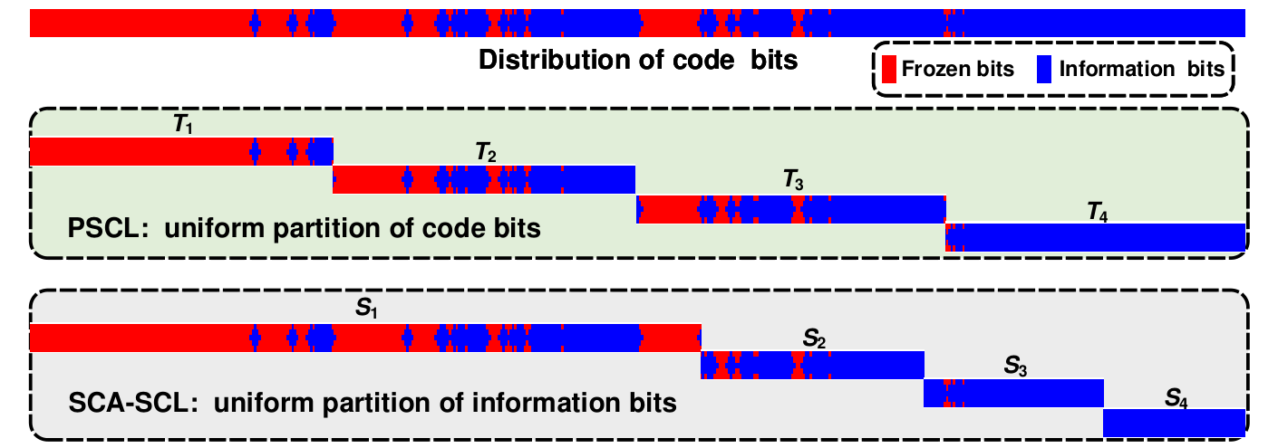
Let $P$ denote the number of segments. For PSCL decoder, the index set of Segment-$i$ is $T_{i}$ ($1\leq i\leq P$). $|\cdot|$ denotes the cardinality of one set. We have

For SCA-SCL decoder, the index set of Segment-$i$ is $S_{i}$ ($1\leq i\leq P$). we have

One simple example of $P=4$ is illustrated in Fig. 5.

Theoretically, both schemes are similar but differ in the partition methods. PSCL decoding employs uniform code bit partition, which is implementation friendly. However, since only one candidate can survive after each CRC, small performance degradation is expected, especially in low SNR region. SCA-SCL decoding employs uniform information bit partition, which can keep the performance as CA-SCL decoding while successfully reducing the space and time complexity. This advantage comes from the decoding flexibility. However, the flexibility will make the implementation more complicated.

The first observation is that, both schemes apply the same CRC to the uniformly partitioned segments. Without looking into the symmetric capacity of each binary channel, this straightforward scheme may not be optimal. The second observation is that both schemes have their own merits, it would be smarter to merge them together. In other words, it is estimated that we can propose a new approach which is both implementation friendly and adaptive.

One simple mixture of both schemes is to introduce early termination to PSCL decoding. However, this simple combination may not be reasonable in certain cases. Fig. 6 gives an example with $P=4$. Shown in Fig. 7, for the $(1024,512)$ code with $m=32$, the information lengths of four segments are $20$, $123$, $156$, and $245$, respectively. If uniform CRC bits are employed, the first segment has $|T^{\prime}_{1}|=|T_{1}|-|C_{1}|=12$ information bits and the last segment has $|T^{\prime}_{4}|=|T_{4}|-|C_{4}|=237$ information bits. It is unreasonable to use the same $8$-bit CRC to both the $12$-bit and $237$-bit segments. To this end, the TCA-SCL decoding is proposed in the following section.

Assume a total of $m$ CRC bits are available and are divided into $P$ segments $C_{1},C_{2},\ldots,C_{P}$. It may not be suitable to set $|C_{1}|=|C_{2}|=\ldots=|C_{P}|$ for $P$ segments with different lengths. How to measure the requirement of the CRC length for each segment is critical. To the authors’ best knowledge, no literature has addressed this specific problem. To maintain the same error detection capability in the situation of independent channels, it is concluded that longer sequence requires more CRC bits [12]. However, this conclusion does not suit polar codes because the reliability of different channels are different. A reasonable measurement on requirement of CRC length should take both sequence length and symmetric capacity into account. In the following, concepts of virtual transform and virtual length are proposed to this end.

Including CRC bits, we always pick the $K+m$ most reliable bits out of $N$ based on the symmetric capacity $I(W^{(i)}_{N})$ with $i\in\mathcal{A^{\prime}}$. $\mathcal{A^{\prime}}$ is the new information set including CRC bits, and $|\mathcal{A^{\prime}}|=K+m$. Calculate $\bar{I}$ as follows:

The CRC allocation is given by

where $\textrm{adjust}(\cdot)$ is a function which adjusts the allocation results to near integers and takes the following steps: 1) find an unmarked $k$ which has minimum $|\textrm{ROUND}(\frac{m\times{v{l_{k}}}}{{\sum\nolimits_{i=1}^{P}{v{l_{i}}}}})-\frac{m\times{v{l_{k}}}}{{\sum\nolimits_{i=1}^{P}{v{l_{i}}}}}|$, then mark $k$ and set $|C_{k}|=\textrm{ROUND}(\frac{m\times{v{l_{k}}}}{{\sum\nolimits_{i=1}^{P}{v{l_{i}}}}})$; 2) repeat step 1) for $(P-2)$ times; 3) Assume the left unmarked index is $k^{\prime}$. Set $|{C_{k^{\prime}}}|=m-\sum\limits_{i\neq k^{\prime}}{|{C_{i}}|}$, where $1\leq i\leq P$.

Before we give more details of the proposed TCA-SCL decoding, one visualization method of symmetric capacity is proposed for easy understanding and illustration. In this visualization, the gradient colors from iridescence are used to demonstrate the symmetric capacity of each channel. According to the legend, the more symmetric capacity approaching $1$ ($0$), the more bathochromic (hypsochromic) it will be. Fig. 8(a) shows the visualization for polar codes with $N=64$.

This refined SCA-SCL decoding based on virtual length is named TCA-SCL decoding. Details of TCA-SCL decoding is given as follows. The corresponding performance and implementation are discussed in Section 6 and Section 7.

The detailed tailored CA-SCL decoding is given in this subsection. For TCA-SCL encoding, we set $P$ segments and perform the virtual transform to obtain the corresponding virtual lengths. Then we allocate the CRC bits according to the ratio of virtual lengths before polar encoding.

Here, $\textrm{addCRC}(\cdot)$ is function which performs Eq. (15). Function $\textrm{encoder}(\cdot)$ performs conventional polar encoding. For TCA-SCL decoding, SCL decoding with early termination is performed as follows. Here, the function $\textrm{SCL}^{\prime}(\cdot)$ is the SCL decoding for Segment-$j$. Define $\mathcal{U}_{i}$ as the the output paths set of SCL($\cdot$) in $i$-th segment. Define $\textrm{passCRC}(\cdot)$ as the function which checks if at least one path of $\mathcal{U}_{i}$ can pass the CRC. If one or more than one path can pass the CRC, the path with the largest metric of them is chosen to refresh $\hat{u}^{N}_{1}$.

In this subsection, performance comparison between different algorithms is given with binary-input additive white Gaussian noise channels (BI-AWGNCs). Different code lengths, rates, and partition schemes are considered: for Fig. 10(a), we have $N=64$, $K=36$, $m=8$, and $P=2$; for Fig. 10(b), we have $N=1024$, $K=512$, $m=32$, and $P=4$. The information set $A$ is selected according to [2, 19]. We use corresponding hex value to represent CRC polynomial. For example, a CRC-$4$ detector with polynomial $g(D)=D^{4}+D+1$ is described as CRC-$4$ ($0$x$9$) in this paper (the ‘$+1$’ is implicit in the hex value). For $(64,36)$ code, we set $2$ copies of CRC-$4$ ($0$x$9$) for (HARQ-)PSCL scheme, and CRC-$5$ ($0$x$12$) and CRC-$3$ ($0$x$5$) for (HARQ-)TCA-SCL scheme. For $(1024,512)$ code, we set $4$ copies of CRC-$8$ ($0$xA$6$) for (HARQ-)PSCL scheme, and CRC-$3$ ($0$x$5$), CRC-$10$ ($0$x$327$), CRC-$11$ ($0$x$583$), and CRC-$8$ ($0$xA$6$) for (HARQ-)TCA-SCL scheme. All the CRC detectors are with the best CRC generation polynomial suggested by [12].

According to Fig. 10, compared with the PSCL scheme, the proposed TCA-SCL scheme has a $0.1$ dB performance gain when $\textrm{FER}=10^{-2}$ for both $(64,36)$ and $(1024,512)$ codes. The HARQ-TCA-SCL ($T=3$) scheme introduces a $0.25$ dB and $0.13$ dB gain over the HARQ-PSCL scheme when frame error rate $\textrm{FER}=10^{-2}$ for $(64,36)$ and $(1024,512)$ codes, respectively.

Define the product of the actual decoding length and list size as the average list size. Since the average computational complexity is proportional to the average list size, here we analyze the average list sizes of TCA-SCL and HARQ-TCA-SCL decoders denoted by $\bar{L}_{T}$ and $\bar{L}_{H}$, respectively. Assume the total frame number is $F$, and the decoder ends at the $P_{i}$-th segment of the $i$-th frame. For the TCA-SCL decoder, $\bar{L}_{T}$ can be calculated as

Suppose the $i$-th frame is retransmitted $R_{i}$ times ($0\leq{R_{i}}\leq T$). For the HARQ-TCA-SCL decoder, $\bar{L}_{H}$ is calculated as

For low SNR, thanks to the early termination $\bar{L}_{T}$ is small due to high error rate. On the other hand, a larger number of retransmissions leads to a higher $\bar{L}_{H}$ for HARQ-TCA-SCL decoder. As SNR increases, $\bar{L}_{T}$ and $\bar{L}_{H}$ converge to $L$: 1) TCA-SCL decoder is more likely to finish the decoding process, and 2) the retransmission time of HARQ-TCA-SCL decoder converges to $0$. It should be noted that, according to Eq. (18) and (19) $0\leq{\bar{L}_{H}}-{\bar{L}_{T}}\leq\frac{L}{P}T$.

Shown in Fig. 11, (HARQ-)TCA-SCL scheme has the same complexity as (HARQ-)PSCL scheme. The HARQ-TCA-SCL scheme has $50.3\%$ and $38.5\%$ higher complexity than the PSCL scheme at $\textrm{SNR}=1.5$ dB for $(64,36)$ and $(1024,512)$ codes, respectively. As SNR goes up, the complexity of HARQ-TCA-SCL scheme tends to be as same as the PSCL scheme asymptotically with better performance.

To better demonstrate the advantages of the proposed TCA-SCL decoders, FPGA implementations based on Altera Stratix V are given as well. To be in accordance with Table 2, five decoders have been implemented. The same parameters as the aforementioned example are employed here: $N=1024$, $K=512$, $m=32$, $P=4$, and $L=2$. All the five decoders employ the same LLR quantization scheme of $1$ sign bit, $6$ integer bits, and $1$ decimal bit. In Fig. 15, the FER performance comparison of floating SC and quantized-SC with $q=8$ bits indicates the validity of the quantized scheme.

The implementation results are compared in terms of adaptive logic modules (ALMs), registers, and memory bits. It is shown that, compared to the CA-SCL decoder, TCA-SCL (SF or DF) decoder can achieve $18.8\%$ or $15.0\%$ ALM reduction. For further ALM reduction, with the help of folding technique, FTCA-SCL (SF or DF) decoder consumes $40.11\%$ or $42.9\%$ ALMs compared to TCA-SCL (SF or DF) with slightly increased latency, as analyzed in [22]. It is also observed that the ALMs’ reduction is not that much as the reduction of MNs listed in Table 1. This is because Table 1 does not consider the comparison part, which introduces major part of ALMs consumption and stays the same between different architectures.

For implementation convenience, here memory has been employed by both folded decoders. Therefore, we consider the sum of registers and memory bits as the total memory consumption. It is observed TCA-SCL (SF or DF) decoder requires $77.03\%$ or $82.1\%$ memory compared to the CA-SCL decoder. Also, the introduction of folding technique does not affect the memory cost, which has been indicated by Theorem 3. Comparing FTCA-SCL (DF) decoder and FTCA-SCL (SF) decoder, when DF scheme is employed, the latency can be reduced $15.90\%$ at the cost of $11.99\%$ increased ALMs.

For the latency issue, since the critical paths of all designs are determined by the critical path of the same SC decoding kernel, we believe it is safe to compare in term of clock number. It is shown that the segmented CRC decoders will introduce more latency due to more serial CRC operations. Second, the DF scheme is more time efficient. Third, the folded versions come at the cost of higher latency.

In general, the proposed four architecture of DC-SCL decoding can reduce the hardware consumption compared to CA-SCL decoder. Designers can choose the suitable one according to different application requirements.

References

- (1) E. Arıkan and E. Telatar, “On the rate of channel polarization,” in Proc. IEEE International Symposium on Information Theory (ISIT), 2009, pp. 1493–1495.
- (2) E. Arıkan, “Channel polarization: A method for constructing capacity-achieving codes for symmetric binary-input memoryless channels,” IEEE Trans. Inf. Theory, vol. 55, no. 7, pp. 3051–3073, July. 2009.
- (3) N. Goela, S. B. Korada, and M. Gastpar, “On LP decoding of polar codes,” in Proc. IEEE Information Theory Workshop (ITW), 2010, pp. 1–5.
- (4) E. Arıkan, “A performance comparison of polar codes and Reed-Muller codes,” IEEE Commun. Lett., vol. 12, no. 6, pp. 447–449, June. 2008.
- (5) N. Hussami, S. B. Korada, and R. Urbanke, “Performance of polar codes for channel and source coding,” in Proc. IEEE International Symposium on Information Theory (ISIT), 2009, pp. 1488–1492.
- (6) I. Tal and A. Vardy, “List decoding of polar codes,” in Proc. IEEE International Symposium on Information Theory Proceedings (ISIT), 2011, pp. 1–5.
- (7) K. Chen, K. Niu, and J. Lin, “List successive cancellation decoding of polar codes,” Electronics Letters, vol. 48, no. 9, pp. 500–501, April 2012.
- (8) K. Niu and K. Chen, “CRC-Aided decoding of polar codes,” IEEE Commun. Lett., vol. 16, no. 10, pp. 1668–1671, 2012.
- (9) E. Arıkan, “Polar Coding for 5G Wireless?” June 2015, Invited Talk of International Workshop on Polar Code.
- (10) H. Zhou, C. Zhang, W. Song, S. Xu, and X. You, “Segmented CRC-Aided SC list polar decoding,” in Proc. IEEE Vehicular Technology Conference (VTC), 2016, pp. 1–5.
- (11) S. A. Hashemi, A. Balatsoukasstimming, P. Giard, C. Thibeault, and W. J. Gross, “Partitioned successive-cancellation list decoding of polar codes,” in Proc. IEEE International Conference on Acoustics, Speech and Signal Processing (ICASSP), 2016, pp. 957–960.
- (12) P. Koopman and T. Chakravarty, “Cyclic redundancy code (CRC) polynomial selection for embedded networks,” in Proc. Annual IEEE/IFIP International Conference on Dependable Systems and Networks (DSN), 2004, pp. 145–154.
- (13) J. Hagenauer, “Rate-compatible punctured convolutional codes (RCPC codes) and their applications,” IEEE Trans. Commun., vol. 36, no. 4, pp. 389–400, 1988.
- (14) D. N. Rowitch and L. B. Milstein, “On the performance of hybrid FEC/ARQ systems using rate compatible punctured turbo (RCPT) codes,” IEEE Trans. Commun., vol. 48, no. 6, pp. 948–959, 2000.
- (15) G. Yue, X. Wang, and M. Madihian, “Design of rate-compatible irregular repeat accumulate codes,” IEEE Trans. Commun., vol. 55, no. 6, pp. 1153–1163, 2007.
- (16) K. Chen, K. Niu, and J. Lin, “A hybrid ARQ scheme based on polar codes,” IEEE Commun. Lett., vol. 17, no. 10, pp. 1996–1999, 2013.
- (17) K. Niu, K. Chen, and J. Lin, “Beyond turbo codes: Rate-compatible punctured polar codes,” in Proc. IEEE International Conference on Communications (ICC), 2013, pp. 3423–3427.
- (18) H. Saber and I. Marsland, “An incremental redundancy hybrid ARQ scheme via puncturing and extending of polar codes,” IEEE Trans. Commun., vol. 63, no. 11, pp. 3964–3973, 2015.
- (19) I. Tal and A. Vardy, “How to construct polar codes,” IEEE Trans. Inf. Theory, vol. 59, no. 10, pp. 6562–6582, 2011.
- (20) C. Zhang, B. Yuan, and K. K. Parhi, “Reduced-Latency SC polar decoder architectures,” in Proc. IEEE International Conference on Communications (ICC), 2011, pp. 3471–3475.
- (21) X. Liang, J. Yang, C. Zhang, W. Song, and X. You, “Hardware efficient and low-latency CA-SCL decoder based on distributed sorting,” in Proc. IEEE Global Communications Conference (GLOBECOM), Dec 2016, pp. 1–6.
- (22) X. Liang, C. Zhang, S. Zhang, and X. You, “Hardware-Efficient folded SC polar decoder based on -segment decomposition,” in Proc. IEEE Asia Pacific Conference on Circuits and Systems (APCCAS), Oct 2016, pp. 1–4.
- (23) S. Lin and D. J. Costello, “Error control coding,” Principles of Mobile Communication, vol. 44, no. 2, pp. 607 – 610, 2004.