A bootstrap test to detect prominent
Granger-causalities across frequencies

Let us suppose that the past values of a time series ${Y}_{t}$, i.e. ${Y}_{t-1}$, ${Y}_{t-2}$, $\dots$, help predicting the value at time $t$ of another time series ${X}_{t}$, that is, ${Y}_{t-1}$, ${Y}_{t-2}$, $\dots$ add significant information to the past values of ${X}_{t}$ (${X}_{t-1}$, ${X}_{t-2}$, $\dots$) for predicting ${X}_{t}$. In that case we say that ${Y}_{t}$ Granger-causes ${X}_{t}$.

We now briefly recall the bases of Granger-causality spectral theory. We follow the approach in Ding et al., (2006), which we refer to for the details. Suppose that ${X}_{t}$ and ${Y}_{t}$, jointly covariance-stationary, follow a non-singular $VAR(k)$ model. Defining $\mathbf{Z}_{t}=[{X}_{t},{Y}_{t}]^{\prime}$, we have

where $\mathbf{\epsilon}_{t}\sim N_{2}(0,{\Sigma_{2}})$, ${\Sigma_{2}}$ is a $2\times 2$ covariance matrix, and $\mathbf{A}_{1},\ldots,\mathbf{A}_{k}$ are $2\times 2$ coefficient matrices.

Moving to the frequency domain, for each frequency $\omega$ we define the transfer function $\mathbf{P}(\omega)$ of $\mathbf{Z}_{t}$ in (2.1) as

which is invertible if and only if the roots of the equation $\det(\mathbf{I}_{p}-\sum_{j=1}^{k}\mathbf{A}_{j}L^{j})\penalty\ =\penalty\ 0$ (where $L$ is the lag operator) lie within the unit circle. Setting $\mathbf{P}(\omega)=$
$\left[\begin{array}[]{cc}P_{{XX}}(\omega)&P_{{XY}}(\omega)\\ P_{{YX}}(\omega)&P_{{YY}}(\omega)\end{array}\right]$, the definition (2.2) allows to define in a compact way the model-based spectrum $h(\omega)$ as follows:

where ^∗ denotes the complex conjugate.

Setting $\mathbf{\Sigma_{2}}=\left[\begin{array}[]{cc}\sigma_{2}&\upsilon_{2}\\ \upsilon_{2}&\gamma_{2}\end{array}\right]$, we need for computational reasons to define the transform matrix $\mathbf{S}=\left[\begin{array}[]{cc}1&0\\ -\frac{\upsilon_{2}}{\gamma_{2}}&1\end{array}\right],$ from which we derive the transformed transfer function matrix $\mathbf{\tilde{{P}}}(\omega)=\mathbf{S}\times\mathbf{P}(\omega)$. The process $\mathbf{Z}_{t}=[{X}_{t},{Y}_{t}]^{\prime}$ is normalized accordingly as $\mathbf{Z}^{*}_{t}=\mathbf{\tilde{{P}}}(L)[{X}_{t},{Y}_{t}]^{\prime}$ and becomes $\mathbf{Z}^{*}_{t}=[{X}^{*}_{t},{Y}^{*}_{t}]^{\prime}$.

The unconditional Granger-causality spectrum of ${X}_{t}$ (effect-variable) respect to ${Y}_{t}$ (cause-variable) is then defined as (Geweke,, 1982)

In the empirical analysis, the theoretical values of coefficient and covariance matrices will be replaced by the corresponding SURE estimates (Zellner,, 1962).

Moreover, we can define the conditional Granger causality spectrum of ${X}_{t}$ respect to ${Y}_{t}$ given an exogenous variable ${W}_{t}$ (conditioning variable). Suppose we estimate a VAR on $[{X}_{t},{W}_{t}]^{\prime}$ with covariance matrix of the noise terms $\mathbf{\Sigma_{2^{\prime}}}=\left[\begin{array}[]{cc}\sigma_{2^{\prime}}&\upsilon_{2^{\prime}}\\ \upsilon_{2^{\prime}}&\gamma_{2^{\prime}}.\end{array}\right]$ and transfer function $\mathbf{G}(\omega)$ (defined as in (2.2)). The corresponding normalized process of $[{X}_{t},{W}_{t}]^{\prime}$ (according to the procedure described above) is denoted by $[{X}^{*}_{t},W^{*}_{t}]^{\prime}$.

We then estimate a VAR on $[{X}_{t},{Y}_{t},{W}_{t}]^{\prime}$ with covariance matrix of the noise terms

and transfer function $\mathbf{P}^{\prime}(\omega)$. Building the matrix

we can define $\mathbf{Q}(\omega)=\mathbf{C}^{-1}(\omega)\mathbf{P}^{\prime}(\omega)$, which is a sort of “conditional” transfer function matrix. The theoretical spectrum of ${X}^{*}$ can thus be written as

The conditional spectrum of ${X}_{t}$ (effect-variable) respect to ${Y}_{t}$ (cause-variable) given ${W}_{t}$ (conditioning variable) is (Geweke,, 1984)

Both $h_{{Y}\rightarrow{X}}(\omega)$ and $h_{{Y}\rightarrow{X}|{W}}(\omega)$ range from $0$ to $\infty$, with $-\pi\penalty\ \leq\penalty\ \omega\penalty\ \leq\penalty\ \pi$. $h_{{Y}\rightarrow{X}}(\omega)$ expresses the power of the relationship from ${Y}$ to ${X}$ at frequency $\omega$, $h_{{Y}\rightarrow{X}|{W}}(\omega)$ expresses the strength of the relationship from ${Y}$ to ${X}$ at frequency $\omega$ given ${W}$. Therefore, the unconditional spectrum accounts for the whole effect of the past values of ${Y}_{t}$ onto ${X}_{t}$, while the conditional spectrum accounts for the direct effect of the past values of ${Y}_{t}$ onto ${X}_{t}$ excluding the effect mediated by the past values of ${W}_{t}$. The same measures are more easily defined in the time-domain. In that case, they are defined for the process as a whole (not frequency-wise as in the frequency domain).

Granger-causality spectra $h_{{Y}\rightarrow{X}}(\omega)$ and $h_{{Y}\rightarrow{X}|W}(\omega)$ can be interpreted as follows. If $h_{{Y}\rightarrow{X}}(\omega)>0$, it means that past values of ${Y}_{t}$ help predicting ${X}_{t}$, and $\frac{1}{\omega}$ is a relevant cycle. If $h_{{Y}\rightarrow{X}|W}(\omega)>0$, it means that past values of ${Y}_{t}$ in addition to those of ${W}_{t}$ help predicting ${X}_{t}$, and $\frac{1}{\omega}$ is a relevant cycle. Significant frequencies give us some hints on the relevant delay structure of the cause variable with respect to the effect variable.

We remark that these measures do not give any information on the sign of the relationship, which is given by time-domain measures like the correlation coefficient. It rather describes the strength, i.e. the intensity, of the causal relationship.

The inference on Granger-causality spectra in the frequency domain is still an open problem. In fact, differently from the corresponding time-domain quantities, the limiting distribution for unconditional and conditional spectra is unknown (see Barnett and Seth, (2014), section 2.5). In spite of that,
Breitung and Candelon, (2006) test the nullity of unconditional and conditional GC at each frequency $\omega$, imposing a necessary and sufficient set of linear restrictions to the (possibly cointegrated) VAR model best fitting the series. The resulting test statistics is distributed under the null as a Fisher distribution with $2$ and $T-2k$ degrees of freedom (except for $\omega=\{0,\pi\}$ at which the distribution is $F_{(1,T-k)}$), where $k$ is the VAR delay and $T$ is the time series length.

As said in the Introduction, that test applied on macroeconomic series often flags most of causalities as significant, due to the rich causality structure. For this reason, in order to disambiguate among significant causalities the most prominent ones, we propose a complementary bootstrap testing approach. At each frequency $\omega$, we test the null hypothesis $H_{0}:t(\omega)=t_{med}$, against the alternative $H_{1}:t(\omega)>t_{med}$, where the functional $t(\omega)$ may be the unconditional GC $h_{{Y}\rightarrow X}(\omega)$, the conditional GC $h_{{Y}\rightarrow{X}|{W}}(\omega)$ or their difference $h_{{Y}\rightarrow X}(\omega)-h_{{Y}\rightarrow{X}|{W}}(\omega)$, and $t_{med}$ is the median of $t(\omega)$ across frequencies under the assumption of stochastic independence.

Since the distributions of $h_{{Y}\rightarrow X}(\omega)$ and $h_{{Y}\rightarrow{X}|{W}}(\omega)$ are unknown, we approximate the distribution of each $t(\omega)$ under the null by the stationary bootstrap of Politis and Romano, (1994). A similar approach was originally proposed by Ding et al., (2006), which tests the same null hypothesis of Breitung and Candelon, (2006) by the randomization procedure of Blair and Karniski, (1993), retaining the maximum causality across frequencies. Differently, our procedure tests by bootstrap the equality between each unconditional or conditional causality and the median causality under the assumption of stochastic independence. Applying the stationary bootstrap to each time series independently of the other ones approximates the no-causality situation, because it approximates the Markov chain best representing independently each series. We stress that unconditional and conditional spectra must be assessed separately, because their distributions are in general different.

In Ding et al., (2006), the comparison between unconditional and conditional Granger causalities is performed using the randomized t-test of Blair and Karniski, (1993) on the bootstrapped series of the causality peak across frequencies. This approach is suitable for their case, where they perform psychological/neurological experiments, which allow to have multiple trials data. On the contrary, in the economic context, we can not perform such a test because we only have a single realization. This is the reason why we take the difference between unconditional and conditional GC, which allows to determine if the conditioning variable has a significant impact (amplification or annihilation) on the causal relationship in our time-dependent data context.

Our idea derives from Politis and Romano, (1994), according to which each Fréchet-differentiable functional may be successfully approximated by the stationary bootstrap, and the resulting bias depends on the sum of the Fréchet-differential $h_{F}$ evaluated at each observation, given that the distance between the empirical and the true distribution function of $X_{t}$ is small.

The bootstrap series obtained via the stationary bootstrap of
Politis and Romano, (1994) are stationary Markov chains conditionally on the data. It means that each bootstrap series $X_{1}^{*},\ldots,X_{T}^{*}$ is a Markov chain conditionally on $X_{1},\ldots,X_{T}$. Suppose that we apply the same procedure to $X_{t}$, $Y_{t}$ and $W_{t}$, obtaining the stationary bootstrap series $X_{t}^{*}$, $Y_{t}^{*}$ and $W_{t}^{*}$. Computing unconditional and conditional Granger causality spectra on those series equals to assess causalities under the assumption of stochastic independence, because the entire stochastic behaviours of $X_{t}^{*}$, $Y_{t}^{*}$ and $W_{t}^{*}$ are explained by the conditional distributions of $X_{t}^{*}|X_{t-1}^{*}$, $Y_{t}^{*}|Y_{t-1}^{*}$, $W_{t}^{*}|W_{t-1}^{*}$. Therefore, testing each Granger-causality computed on the original series $X_{t}$, $Y_{t}$ and $W_{t}$ against the median causality computed across frequencies on $X_{t}^{*}$, $Y_{t}^{*}$ and $W_{t}^{*}$ is effective as a test for causality strength in relative terms.

Let us consider $\hat{r}(\omega)=\hat{h}_{{Y}\rightarrow X}(\omega)$, which is defined as (2.3) where the coefficient matrices $\mathbf{A}_{j},j=1,\ldots,k$, and the error covariance matrix $\mathbf{\Sigma_{2}}$ are replaced by the corresponding SURE estimates (Zellner,, 1962). We know that SURE estimates $\mathbf{\hat{A}}_{j}$, $j=1,\ldots,k$, are rational functions of the data, thus being Fréchet-differentiable. $\mathbf{\hat{\tilde{{P}}}}(\omega)$ and $\mathbf{\hat{\Sigma}}_{2}$ are functions of the $\mathbf{\hat{A}}_{j}$, thus being rational in turn; the same holds as a consequence for $\hat{{{h}}}(\omega)$. Therefore, $\hat{h}_{{Y}\rightarrow X}(\omega)$, the natural logarithm of a rational function of the data, is Fréchet-differentiable. At this point, as pointed out in Politis et al., (2012), page 30, even if the median is not Fréchet-differentiable, the bootstrap for $\hat{h}_{{Y}\rightarrow X}(\omega)$ is still valid, provided that the density function of $median({h}_{{Y}\rightarrow X}(\omega))$ is positive. As a consequence, according to Politis and Romano, (1994), paragraph 4.3, we can estimate consistently any quantile of the distribution of the median of $\hat{h}_{{Y}\rightarrow X}(\omega)$ under the null hypothesis.

Considering $\hat{r}(\omega)=\hat{h}_{{Y}\rightarrow{X}|{W}}(\omega)$, which is defined as (2.4) where the coefficient matrices and the error covariance matrix are replaced by the corresponding SURE estimates, a similar reasoning can be carried out. The same applies to the estimated difference of $\hat{h}_{{Y}\rightarrow X}(\omega)-\hat{h}_{{Y}\rightarrow{X}|{W}}(\omega)$, that is Fréchet-differentiable apart from the case $\hat{h}_{{Y}\rightarrow X}(\omega)=\hat{h}_{{Y}\rightarrow{X}|{W}}(\omega)$, which holds with null probability.

We stress that our aim is not to represent the common multivariate distribution function $F$ of the process $\mathbf{Z}_{t}=[X_{t},Y_{t},W_{t}]$. That problem is an estimation one, which would be effectively solved by parametric or residual bootstrap. Our aim is to exploit the random process $\mathbf{Z}_{t}^{*}=[X_{t}^{*},Y_{t}^{*},W_{t}^{*}]$ to derive the bootstrap quantile $q_{1-\alpha}^{*}$ which satisfies

where $\alpha$ is the significance level and $r_{med}^{*}$ is the bootstrap median across frequencies of unconditional, conditional GC or their difference under the assumption of stochastic independence. Since $r_{med}$ is Fréchet-differentiable, $P(r_{med}^{*}\leq q_{1-\alpha}^{*})$ approximates consistently $P(r_{med}\leq q_{r,1-\alpha})$ as $T^{\frac{1}{3}}\rightarrow\infty$ under the null hypothesis of stochastic independence.

In more detail, suppose that $r$ is a Fréchet-differentiable functional, that is, there exists some influence function $h_{F}$ such that

with $\int h_{F}dF=0$ ($||.||$ is the supremum norm). We define the mixing coefficient

where $A$ and $B$ vary over events in the $\sigma$-fields generated by $\{X_{t},t\leq 0\}$ $\{X_{t},t\geq k\}$. The following Theorem holds.

We refer to Appendix Appendix for the proof.

Due to the nature of our test, we need to exclude any stochastic process with a constant Granger-causality spectrum different from a white noise. Suppose that $\mathbf{Z}_{t}$ is a stochastic process with auto-covariance matrices $\mathbf{R}_{j}=cov(\mathbf{Z}_{t},\mathbf{Z}_{t-j})$, $j\in\mathcal{Z}^{+}$. Throughout the paper, we need to assume that, in case there is at least one non-zero causality coefficient at one delay $j\in\mathcal{Z}^{+}$, the resulting covariance matrix is not diagonal, i.e. the effect and the cause variable are not uncorrelated. At the same time, we need to assume that each auto-covariance matrix $R_{j}$, $j\geq 1$, is positive definite.

We clarify the expressed constraints by an example. Consider the case of a $VAR(1)$ with the following parameters: $\mathbf{\Sigma}=diag(1,1)$, $\mathbf{A}_{1}=\left[\begin{array}[]{cc}0&0.5\\ 0&0\end{array}\right]$. According to Wei et al., (2006), p. 392, the vectorized covariance matrix of a vector $AR(1)$ process is $vec(R_{0})=(\mathbf{I}-\mathbf{A}_{1}\otimes\mathbf{A}_{1})^{-1}vec(\mathbf{\Sigma})$ and the vectorized autocovariance matrix at lag $k$ is $vec(\mathbf{R}_{k})=vec(\mathbf{R}_{0})\mathbf{A}_{1}^{k}$. Therefore, we have $\mathbf{R}_{0}=diag(1.25,1)$, while $\mathbf{R}_{1}$, $\mathbf{R}_{2}$, $\ldots$ are singular matrices. The same holds, for instance, if we suppose $\mathbf{A}_{1}=\left[\begin{array}[]{cc}0.5&0.5\\ 0&0\end{array}\right]$. In that case, the covariance matrix results $\mathbf{R}_{0}=diag(\frac{5}{3},1)$.

Such cases cannot be dealt by our procedure, as SURE estimates are inconsistent. Out of this pathological set, our test achieves a power of $100\%$ if the underlying process is non-stationary. On the contrary, the test of
Breitung and Candelon, (2006) is less conservative, flagging surely as significant any causality distant enough from $0$.

We now report in detail the testing procedures relative to the three functionals.

• •

  For the functional $\hat{h}_{{Y}\rightarrow X}(\omega)$, our bootstrap procedure is

  • –

    Simulate $N$ stationary bootstrap series $(X^{*}_{t},Y^{*}_{t})$ given the observed series $(X_{t},Y_{t})$.

  • –

    On each simulated series $(X^{*}_{t},Y^{*}_{t})$:

    1. 1.

       estimate a VAR model on $(X^{*}_{t},Y^{*}_{t})$ via SURE using BIC for model selection.

    2. 2.

       at Fourier frequencies $f_{i}=\frac{i}{T},i=1,\ldots,[\frac{T}{2}]$, compute $h_{{Y^{*}}\rightarrow X^{*}}(2\pi f_{i})$.

    3. 3.

       compute $median_{\{f_{i},i=1,\ldots,T/2\}}h_{{Y^{*}}\rightarrow X^{*}}(2\pi f_{i})$.

  • –

    Then, compute $q_{uncond,1-\alpha}$, the $(1-\alpha)$-quantile of the bootstrap distribution at Step 3 across the $N$ bootstrap series, where $\alpha$ is the significance level.

  • –

    Finally, at each $f_{i}$, flag $\hat{h}_{{Y}\rightarrow X}(2\pi f_{i})$ as significant if larger than $q_{uncond,\alpha}$.

• •

  For the functional $\hat{h}_{{Y}\rightarrow{X}|{W}}(\omega)$, the procedure becomes

  • –

    Simulate $N$ stationary bootstrap series $(X^{*}_{t},Y^{*}_{t},W^{*}_{t})$ given the observed series $(X_{t},Y_{t},W_{t})$.

  • –

    On each simulated series $(X^{*}_{t},Y^{*}_{t},W^{*}_{t})$:

    1. 1.

       estimate a VAR model on $(X^{*}_{t},W_{t}^{*})$ and $(X^{*}_{t},Y^{*}_{t},W^{*}_{t})$ via SURE using BIC for model selection.

    2. 2.

       at Fourier frequencies $f_{i}=\frac{i}{T},i=1,\ldots,[\frac{T}{2}]$, compute $h_{{Y^{*}}\rightarrow{X^{*}}|{W^{*}}}(2\pi f_{i})$.

    3. 3.

       compute $median_{\{f_{i},i=1,\ldots,T/2\}}h_{{Y^{*}}\rightarrow{X^{*}}|{W^{*}}}(2\pi f_{i})$.

  • –

    Then, compute $q_{cond,1-\alpha}$, the $(1-\alpha)$-quantile of the bootstrap distribution at Step 3 across the $N$ bootstrap series.

  • –

    Finally, at each $f_{i}$, flag $\hat{h}_{{Y}\rightarrow{X}|{W}}(2\pi f_{i})$ as significant if larger than $q_{cond,\alpha}$.

• •

  For the functional $\hat{h}_{{Y}\rightarrow X}(\omega)-\hat{h}_{{Y}\rightarrow{X}|{W}}(\omega)$, the procedure is

  • –

    Simulate $N$ stationary bootstrap series $(X^{*}_{t},Y^{*}_{t},W^{*}_{t})$ given the observed series $(X_{t},Y_{t},W_{t})$.

  • –

    On each simulated series $(X^{*}_{t},Y^{*}_{t},W^{*}_{t})$:

    1. 1.

       estimate a VAR model on $(X^{*}_{t},Y^{*}_{t})$, $(X^{*}_{t},W^{*}_{t})$ and $(X^{*}_{t},Y^{*}_{t},W^{*}_{t})$ via SURE using BIC for model selection.

    2. 2.

       at Fourier frequencies $f_{i}=\frac{i}{T},i=1,\ldots,[\frac{T}{2}]$, compute $h_{{Y^{*}}\rightarrow X^{*}}(2\pi f_{i})-h_{{Y^{*}}\rightarrow{X^{*}}|{W^{*}}}(2\pi f_{i})$.

    3. 3.

       compute $median_{\{f_{i},i=1,\ldots,T/2\}}h_{{Y^{*}}\rightarrow X^{*}}(2\pi f_{i})-h_{{Y^{*}}\rightarrow{X^{*}}|{W^{*}}}(2\pi f_{i})$.

  • –

    Then, compute $q_{diff,\frac{\alpha}{2}}$ and $q_{diff,1-\frac{\alpha}{2}}$, the $(\frac{\alpha}{2})$- and $(1-\frac{\alpha}{2})$-quantiles of the bootstrap distribution at Step 3 across the $N$ bootstrap series.

  • –

    Finally, at each $f_{i}$, flag $\hat{h}_{{Y}\rightarrow X}(2\pi f_{i})-\hat{h}_{{Y}\rightarrow{X}|{W}}(2\pi f_{i})$ as significant if smaller than $q_{diff,\frac{\alpha}{2}}$ or larger than $q_{diff,1-\frac{\alpha}{2}}$.

We provide an R package, called “grangers”, which performs these routines.

In addition, we extend our framework to test the nullity of $r(2\pi f_{i})$, $i=1,\ldots,[\frac{T}{2}]$, across the frequency range. In order to do that, we apply Bonferroni correction, that is, we apply the test procedure to each frequency with significance level $\frac{2\alpha}{T}$. In this way, we ensure that the overall level is not larger than $\alpha$ under the null. This approach is conservative: anyway, the test still has a power of $100\%$ as the VAR process tends to non-stationarity.

In order to clarify the interpretation of our results, we need to define the concept of “prominence” in a formal way. At a significance level $\alpha$, given a random time series sampled by the underlying data generating process, any functional $r(\omega)$ is said to be maximally prominent at frequency $\omega$ if $P\{r(\omega)>r_{med}\}>1-\alpha$, where $r_{med}$ is the median of $r(\omega)$ across frequencies. As a consequence, the power of our test procedure approaches $1$ as $r(\omega)$ is maximally prominent.

We define the prominence rate at frequency $\omega$ as the expected probability of $r(\omega)$ to be maximally prominent: $prom(\omega)$: $P(r(\omega)>q_{1-\alpha})$. The prominence rate answers the question “Which is the probability that $r(\omega)$ is maximally prominent?” The degree of prominence at frequency $\omega$ is then defined as $dp(\omega)$: $P(r(\omega)>r_{med})$. Instead, the power at frequency $\omega$ is defined as $power(\omega)=P(\hat{r}(\omega)>q_{1-\alpha})$. Denoting the solutions of the characteristic equation $\det(\mathbf{I}_{p}-\sum_{j=1}^{k}\mathbf{A}_{j}L^{j})\penalty\ =\penalty\ 0$ in decreasing order by $\lambda_{1},\ldots,\lambda_{q}$, the maximal power at frequency $\omega$ is defined as $mp(\omega)=\lim_{|\lambda_{1}|\rightarrow 1}power(\omega)$. For our test we observe $\max_{\omega\in]0,2\pi]}mp(\omega)=1$.

In general, $\hat{r}(\omega)$ is significant if larger than ${r}_{med}^{*}$ at a significance level $\alpha$. As explained in Section 2.2, the distribution of ${r}_{med}^{*}$ consistently resembles the one of ${r}_{med}$ by the stationary bootstrap. The level of our test, as expected, is approximately equal to the chosen significance level $\alpha$ under the null, i.e. in case of zero-causality at all frequencies (white noise process).

We now describe the performance of our test in a number of situations. First of all, suppose that we simulate $100$ replicates from a VAR process in the form (2.1) with $k=1$, $\mathbf{\Sigma}=diag(1,1)$ and no causality coefficients. The VAR delay is selected for each bootstrap setting by BIC criterion. Our tested coefficient matrix $\mathbf{A}_{1}$ is ${A_{1,(jj)}}=0,0.2,0.5,0.8,1$, $j=1,2$. We observe that the estimated level is below $5\%$ at all Fourier frequencies, as long as $A_{1,(jj)}$ is distant from $1$. If $A_{1,(jj)}=1$ (double random walk), the rejection rate increases at low frequencies, according to the shape of prominence rate and degree of prominence, until $0.4$.

Another relevant case we deal with is for $k=1$ and ${A_{1,(j2)}}=0.5,1$, $j=1,2$. This process has an unconditional causality which decreases as the frequency increases. For ${A_{1,(j2)}}=0.5$ (Figure 2), the degree of prominence ranges from $0.8$ to $0.3$ and the rejection rate is above $5\%$ at all frequencies, ranging from $0.9$ to $0.3$ approximately. For ${A_{1,(j2)}}=1$ (Figure 2), the power at the lowest frequency is one, reflecting the prominence rate and the degree of prominence.

The same case is tested for the conditional causality, with very similar results.

We now compare an unconditional and a conditional causality which are zero at all frequencies. For both cases, the rejection rates stand below $5\%$ at all frequencies. If we compare two decreasing causalities having the shape above described (${A_{1,(j2)}}=0.5,1$, $j=1,2$), the rejection rate at the lowest frequency tends to increase until $0.4$ if the non-zero coefficients are equal to $1$ (the limit case of a double random-walk). This pattern reflects the shape of prominence rate and degree of prominence (Figure 4).

If we compare an unconditional null causality to a decreasing conditional causality with parameters $0.5$ and $1$, the rejection rate is above $5\%$ at all frequencies and increases to $0.6$ or to $1$ respectively at the lowest frequency. In the latter case, we are in presence of a maximally prominent causality difference, as the degree of prominence and the prominence rate confirm.

Moreover, consider the VAR models described in Breitung and Candelon, (2006), paragraph 4. Those models have $k=3$, ${A_{k,(j2)}}=1$, $k=1,3$, $j=1$ and ${A_{k,(j2)}}=-2\cos(\omega^{*})$, $k=2$, $j=1$. Such coefficient structure results in a null causality at frequency $\omega^{*}$. On these settings, we can compare the results of our test to the results of “BC test” by Breitung and Candelon, (2006), which appear in dashed line. In addition, we test the sensitivity of the results to the condition number of the covariance matrix, setting $\mathbf{\Sigma}=diag(1,1)$, $\mathbf{\Sigma}=diag(0.2,1)$, $\mathbf{\Sigma}=diag(5,1)$.

If $\omega^{*}=\frac{\pi}{2}$ and $\mathbf{\Sigma}=diag(1,1)$, our rejection rate is $0.8$ at extreme frequencies, and $0.6$ at $\omega^{*}$, resembling the shape of the degree of prominence (Figure 5). On the contrary, BC test shows a rejection rate of $0.2$ at $\omega^{*}$, and $1$ at extreme frequencies. Setting $\mathbf{\Sigma}=\mathbf{diag}(0.2,1)$, the rejection rate of BC test ranges from $0.7$ to $0.2$, while ours is approximately constant around $0.3$ (Figure 6). This happens because the magnitude of $X$ is much smaller than the one of $Y$, such that $X$ is close to a null process, and the underlying causality is small and detected as constant across frequencies. Setting $\mathbf{\Sigma}=diag(5,1)$ (Figure 7), the rejection rate of both tests stands around $1$, except from a value of $0.3$ at $\omega^{*}$. This occurs because the magnitude of $Y$ is much smaller than the one of $X$, such that any non-null causality is detected as maximally prominent.

Setting $A_{k,(22)}$, $k=1,3$, to $0.25$ and $0.5$ equals to increase the magnitude of the VAR roots until the limit value of $1$ (non-stationary case). In that case, we observe that the range of our rejection rate increases accordingly to the degree of prominence, achieving $1$ in the non-stationary case. Our competitor detects much better the null causality, while it is less able, as expected, to catch the shape of the degree of prominence across frequencies.

If we set, as in Breitung and Candelon, (2006), $\omega^{*}=0$, $\omega^{*}=\frac{\pi}{4}$, $\omega^{*}=\frac{3\pi}{4}$ and $\omega^{*}={\pi}$, we note that our competitor is less precise, as described therein, particularly for the first two cases, because the rejection rate is considerably above $5\%$. Its rejection rate for non-zero causalities is $100\%$, while ours resembles the shape of the degree of prominence, which tends to $0$ for null causalities with particular intensity for the cases $\omega^{*}=0$, $\omega^{*}=1$.

To sum up, the rejection rate of our test depends on three factors:

• •

  the magnitude of VAR roots, which has the effect to extend the range. In general, the rejection rate is perturbed at low frequencies as the process is closer to non-stationarity;

• •

  the true underlying spectral variability, which in turn depends on the relationship between the magnitude of causality and non-causality coefficients;

• •

  the condition number of the autocovariance matrices $\mathbf{R}_{j}$, $j\geq 0$, which masks the underlying spectral variability.

In Table 1 we report the rejection rates of the test on all causalities jointly considered obtained by Bonferroni correction. We note that the test has power approximately $0.05$ in case of no-causality (Case 3), and approximately $1$ in case of non-stationarity (Cases 2 and 7).

We have considered the time series of GDP at market price in the Euro Area (chain linked volumes in Euro) and the monetary aggregate M3 and M1 (outstanding amount of loans to the whole economy excluded the monetary and financial sector, all currencies combined). M3 is also called “broad money”, M1 “narrow money”.

There is not a general consensus on which measure of money supply is the most appropriate. While the Federal Reserve has officially ceased to publish M3 series since 2006, the M3 index of notional stocks, i.e. the annual growth rate of the outstanding amount (also called “base money”), is still used by the ECB as the official measure of short-term circulating money. For a nice discussion on the role of M3 as a policy target for central bankers see for example Alves et al., (2007).

Since our goal is to focus on the effect of monetary policy on output, we restrict our analysis to the period 1999-2017, when the ECB has taken actual decisions on the Euro Area. Monthly series (all but GDP) are made quarterly by averaging. We can thus denote our series by ${GDP}_{t}$, ${M3}_{t}$, ${M1}_{t}$, ${HICP}_{t}$, ${UN}_{t}$, ${LTN}_{t}$, where $t=1,\ldots,56$ (there are $56$ quarters from Winter 2001 to Autumn 2014). The data are drawn from the ECB Real Time Research database where national figures are aggregated according to a changing composition of the Euro Area across time (see Giannone et al., (2012)). We refer to https://www.ecb.europa.eu/stats and ECB, (2012) for technical and computational details.

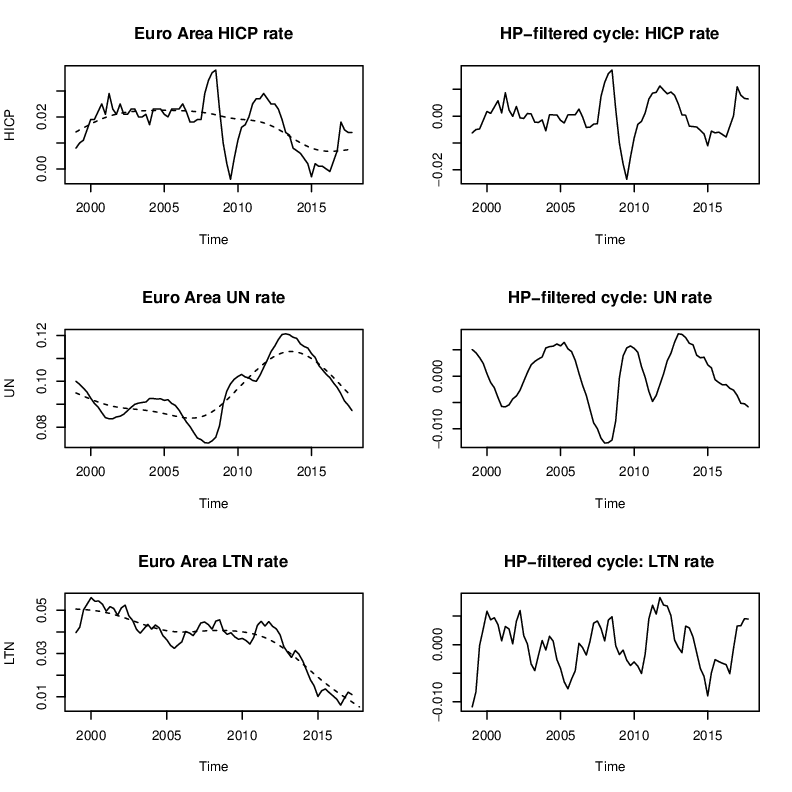
According to Dickey-Fuller test, the logarithmic transform of $GDP_{t}$, $M3_{t}$, $M1_{t}$ are non-stationary, as well as the three conditioning variables $HICP_{t}$, $UN_{t}$ and $LTN_{t}$. Therefore, following Friedman and Schwartz, (1975), we pass all series by Hodrick-Prescott filter (Hodrick and Prescott,, 1997), with the canonical value of $\lambda=1600$, in order to remove any trend and to extract cyclical components. We do not use Baxter-King filter (Baxter and King,, 1999), as suggested in Belongia and Ireland, (2016), because we have not enough end of sample data. Cycle extraction is performed via the R package “mFilter”.

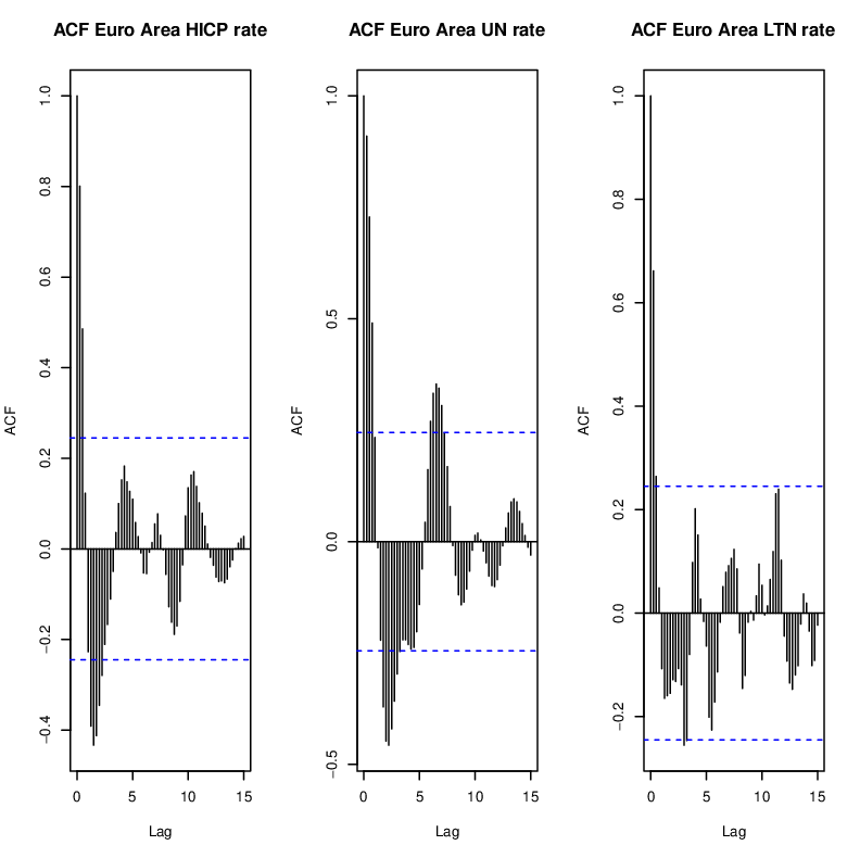
Figures 9 and 9 contain the plots of $GDP_{t}$, $M3_{t}$, $M1_{t}$ and $HICP_{t}$, $UN_{t}$, $LTN_{t}$ respectively. Left figures contain the original series and the estimated trend, while right figures contain the estimated cycles. Figures 11 and 11 show the ACF of the extracted cycles. The patterns are very similar across series: positive for the first 4-5 quarters, negative for all quarters around 2 years and non-significant elsewhere. $UN_{t}$ shows a rebound for the quarters around $5$ years. $LTN_{t}$ is no longer significant after $2$ quarters. Figure 12 shows the CCF for the couples GDP-M3 and GDP-M1. Their pattern is similar: we have positive correlation around $0$ and negative correlation at sides around the lag of $2$ years.

Since our ultimate goal is to infer about the cause-effect relationship of money stock and economic output, we test at each frequency the equality between Granger-causality spectra and the median GC across frequencies, both unconditional and conditional on the inflation rate, the unemployment rate and the long-term interest rate. In this way, we can display the relevant cycles in the causality structure of the relationship from GDP to M3 (M1) and viceversa. Due to the use of Fast Fourier Transform, the frequencies used are the following: $f_{i}=\frac{i}{80},i=1,\ldots,40$, because $T=76$. The frequency range is re-scaled to $[0,2]$ for the quarterly frequency of our series.

Relevant VAR models, estimated including an intercept by the R package “vars” (Pfaff et al.,, 2008), are selected by the Bayesian Information Criterion (BIC), imposing a maximum of four lags. BIC is used because we know that BIC is correctly estimating the unknown number of delays, while AIC may overestimate it, thus increasing the probability to estimate non-stationary VAR models. In any case, all roots of estimated characteristic polynomials are strictly smaller than one. In the end, the resulting number of delays is then fixed across the bootstrap inference procedure for each VAR estimation. The number of bootstrap samples is $1000$.

Note that for computational reasons BC test cannot be computed for $k=1$. Besides, its p-value is constant across frequencies (except the last one) for $k=2$. BC test requires a large number of delays, while ours works for all values, given that the resulting VAR is stationary and non-singular. Therefore, we can not compare directly our test to BC test on real data, because BC is not useful for all cases with $k\leq 2$.

We start describing VAR estimates on the couple GDP-M3. Our lag selection procedure chooses $2$ lags. In the ${GDP}_{t}$ equation, ${GDP}_{t-1}$ and ${GDP}_{t-2}$ are heavily significant, while ${M3}_{t-1}$ and ${M3}_{t-2}$ slightly are (at $5\%$ and $10\%$ respectively). This results in a GC spectral shape which is approximately constant across frequencies. In the ${M3}_{t}$ equation, $M3_{t-1}$ is heavily significant, while $GDP_{t-2}$ is at $10\%$. The corresponding GC shape is prominent at low frequencies.

Concerning the couple GDP-M1, our VAR lag selection procedure chooses $2$ lags. In the ${GDP}_{t}$ equation, ${GDP}_{t-1}$, ${GDP}_{t-2}$ and ${M1}_{t-2}$ are heavily significant. The related unconditional GC shape is prominent at low frequencies only. In the ${M1}_{t}$ equation, only ${M1}_{t-1}$ is heavily significant, while $GDP_{t-1}$ has a p-value of $12\%$. The resulting GC spectral shape is thus prominent only at very low frequencies.

In Figures 14 and 14, unconditional and conditional GC spectra from M3 to GDP and viceversa are reported. The same spectra from M1 to GDP and viceversa are reported in Figures 16 and 16 respectively. In dashed the bootstrap threshold at 5% is outlined. In dotted, the same threshold for the overall test obtained by Bonferroni correction is depicted.

We first comment conditional GC spectra for the couple GDP-M3. Conditioning on HICP, the level of significance of ${M3}_{t-1}$ and ${M3}_{t-2}$ is increased in the ${GDP}_{t}$ equation. This results in a GC decreasing across frequencies and prominent across the entire frequency range. In the $M3_{t}$ equation, the level of significance of ${GDP}_{t-2}$ increases to $5\%$. As a result, GC is prominent until the period of $1$ year. Conditioning on UN, in the ${GDP}_{t}$ equation the level of significance of ${M3}_{t-1}$ is $5\%$ while ${M3}_{t-2}$ is no longer significant. This results in a GC prominent only across the left half of the frequency range. In the $M3_{t}$ equation, ${GDP}_{t-2}$ is no longer significant, resulting in a non-prominent GC everywhere. Conditioning on LTN, the level of significance is $5\%$ for ${M3}_{t-1}$ and $10\%$ for ${M3}_{t-2}$ in the $GDP_{t}$ equation. The corresponding GC is prominent across the entire frequency range. In the $M3_{t}$ equation, ${GDP}_{t-2}$ is significant at $5\%$, causing again GC to be prominent everywhere.

We now comment conditional GC spectra for the couple GDP-M1. Conditioning on HICP, in the $GDP_{t}$ equation ${M1}_{t-2}$ is still heavily significant. The spectral shape is almost the same as the unconditional one. In the $M1_{t}$ equation, the level of significance is quite smaller, so that the only prominent causality is at the lowest frequency. Conditioning on UN, ${M1}_{t-2}$ is still heavily significant in the $GDP_{t}$ equation. The spectral shape is very close to the unconditional one (even if slightly weaker). In the $M1_{t}$ equation, $GDP_{t-1}$ has a p-value of $20\%$ and the related GC shape is close to the unconditional one. Conditioning on LTN, ${M1}_{t-2}$ is still significant at $1\%$ in the $GDP_{t}$ equation, causing GC shape to be almost the same as the one conditioning on UN. In the $M1_{t}$ equation, $GDP_{t-1}$ has a p-value of $26\%$. As a consequence, we observe prominence only at the lowest frequency.

Concerning the overall test on all causalities, we observe the absence of any significance in four cases out of sixteen: the GC spectra from M3 to GDP, unconditional and conditional both on UN and LTN, and the GC spectrum from GDP to M3 conditional on UN. We remark that this test is conservative in nature: however, it allows to adequately contextualize the significance of individual tests.

Finally, GC spectral differences are reported in Figures 18, 18 for the couple $M3-GDP$, in Figures 20, 20 for the couple $M1-GDP$ . From M3 to GDP, we only observe a remarkable amplification power of HICP at low frequencies. UN and LTN show no-causality influence even according to the overall test. From GDP to M3, HICP and LTN show amplification power at the lowest frequency and annihilation power around the period of 2 years. On the contrary, UN amplifies the causal relationship across the left quarter of the frequency range. From M1 to GDP, the three conditioning variables show annihilation power at very low frequencies. From GDP to M1, UN is observed to amplify the link at low frequencies, while the impact of HICP and LTN is not remarkable even according to the overall test.

To sum up, the causal relationship from M3 to GDP is prominent only conditionally on HICP, which appears to be an amplifier, at low frequencies. We can say that conditionally on HICP the low frequency components of M3 appear to be good predictors of the same components of GDP one step ahead. The causal relationship from GDP to M3 is also present at low frequencies, except if we condition on UN, which shows a strong annihilation power. On the contrary, the causality from M1 to GDP is prominent, both unconditionally and conditionally on HICP, UN and LTN, at all frequencies. The three explanatory variables show a remarkable annihilation power at low frequencies. In the end, the causality from GDP to M1 appears strong at low frequencies only. The impact of HICP and LTN on the link can be assumed to be non-remarkable, while UN shows a remarkable amplification power at very low frequencies.

Let us define the random vector $\mathbf{Z}_{t}=[X_{t},Y_{t},W_{t}]$. We assume that $X_{t}$, $Y_{t}$ and $Z_{t}$ are stochastically independent, which causes the null hypothesis of no-causality to hold. This is like assuming that the distribution function $F_{\mathbf{Z}}$ can be factorized as $F_{X}F_{Y}F_{W}$. In addition, we assume that $X_{t}$, $Y_{t}$ and $Z_{t}$ are strictly stationary.

By Politis and Romano, (1994) (paragraph 4.3) we know that

where $\hat{F}_{X}$ is the empirical density function of $X_{t}$ and $F_{X}$ is the corresponding true distribution function. The same equation holds for $Y$ and $Z$.

If, for some $d\geq 0$, $E(h_{F_{X}}(X_{1}))^{2+d}<\infty$, and if it holds $\sum_{k}\alpha_{X}(k)^{\frac{d}{2+d}}<\infty$, then $\frac{1}{\sqrt{T}}\sum_{i=1}^{T}h_{F_{X}}(X_{i})$ is asymptotically normal with mean $0$ and variance

The same equation holds for $Y$ and $W$ if $E(h_{F_{Y}}(Y_{1}))^{2+d}$, $\alpha_{Y}(k)^{\frac{d}{2+d}}<\infty$, and $E(h_{F_{W}}(W_{1}))^{2+d}$, $\sum_{k}\alpha_{W}(k)^{\frac{d}{2+d}}<\infty$ respectively.

At the same time, if $\sum_{k}k^{2}\alpha_{X}(k)^{1/2-\tau}<\infty$, $\sum_{k}k^{2}\alpha_{Y}(k)^{1/2-\tau}<\infty$,
$\sum_{k}k^{2}\alpha_{Z}(k)^{1/2-\tau}<\infty$ for some $0<\tau<1/2$, the stochastic processes $\hat{F}_{X}-F_{X}$, $\hat{F}_{Y}-F_{Y}$, $\hat{F}_{W}-F_{W}$ converge in supremum norm to a Gaussian process having continuous paths and mean $0$. Therefore, $\sqrt{T}(r(\hat{F})-r(F))$ is asymptotically normal with mean $0$ and variance (4.2).

Moreover, for each random variable the distribution of $\sqrt{T}(r(\hat{F})-r(F))$ is approximated via the distribution of $\sqrt{T}(r(\hat{F}^{*})-r(\hat{F}))$, where $\hat{F}^{*}$ is the empirical density function obtained via stationary bootstrap. This holds because the two distributions converge to the same Gaussian process under previous weak dependence assumptions, provided that $T^{\frac{1}{3}}\rightarrow\infty$.

References

- Alves et al., (2007) Alves, N., Marques, C. R., Sousa, J., et al. (2007). Is the euro area m3 abandoning us? Technical report.
- Andrés et al., (2006) Andrés, J., David López-Salido, J., and Vallés, J. (2006). Money in an estimated business cycle model of the euro area. The Economic Journal, 116:457–477.
- Assenmacher-Wesche and Gerlach, (2008) Assenmacher-Wesche, K. and Gerlach, S. (2008). Interpreting euro area inflation at high and low frequencies. European Economic Review, 52:964–986.
- Barnett and Seth, (2014) Barnett, L. and Seth, A. K. (2014). The mvgc multivariate granger causality toolbox: a new approach to granger-causal inference. Journal of neuroscience methods, 223:50–68.
- Baxter and King, (1999) Baxter, M. and King, R. G. (1999). Measuring business cycles: approximate band-pass filters for economic time series. the Review of Economics and Statistics, 81(4):575–593.
- Belongia and Ireland, (2016) Belongia, M. T. and Ireland, P. N. (2016). Money and output: Friedman and schwartz revisited. Journal of Money, Credit and Banking, 48(6):1223–1266.
- Berger and Osterholm, (2011) Berger, H. and Osterholm, P. (2011). Does money growth granger cause inflation in the euro area? evidence from out‐of‐sample forecasts using bayesian vars. Economic Record, 87:45–60.
- Berzuini et al., (2012) Berzuini, C., Dawid, P., and Bernardinelli, L. (2012). Causality: Statistical perspectives and applications. John Wiley & Sons.
- Blair and Karniski, (1993) Blair, R. C. and Karniski, W. (1993). An alternative method for significance testing of waveform difference potentials. Psychophysiology, 30(5):518–524.
- Breitung and Candelon, (2006) Breitung, J. and Candelon, B. (2006). Testing for short-and long-run causality: A frequency-domain approach. Journal of Econometrics, 132:363–378.
- Brovelli et al., (2004) Brovelli, A., Ding, M., Ledberg, A., Chen, Y., Nakamura, R., and Bressler, S. L. (2004). Beta oscillations in a large-scale sensorimotor cortical network: directional influences revealed by granger causality. Proceedings of the National Academy of Sciences of the United States of America, 101:9849–9854.
- Canova and Menz, (2011) Canova, F. and Menz, T. (2011). Does money matter in shaping domestic business cycles? an international investigation. Journal of Money, Credit and Banking, 43:577–607.
- Cendejas et al., (2014) Cendejas, J. L., Castañeda, J. E., and Muñoz, F.-F. (2014). Business cycle, interest rate and money in the euro area: A common factor model. Economic Modelling, 43:136–141.
- Dhamala et al., (2008) Dhamala, M., Rangarajan, G., and Ding, M. (2008). Analyzing information flow in brain networks with nonparametric granger causality. Neuroimage, 41:354–362.
- Ding et al., (2006) Ding, M., Chen, Y., and Bressler, S. L. (2006). 17 granger causality: Basic theory and application to neuroscience. Handbook of time series analysis: recent theoretical developments and applications, page 437.
- ECB, (2012) ECB (2012). Manual on mfi balance sheet statistics, april 2012.
- Friedman and Schwartz, (1975) Friedman, M. and Schwartz, A. J. (1975). Money and business cycles. In The state of monetary economics, pages 32–78. NBER.
- Friedman and Schwartz, (2008) Friedman, M. and Schwartz, A. J. (2008). A monetary history of the United States, 1867-1960. Princeton University Press.
- Geweke, (1982) Geweke, J. F. (1982). Measurement of linear dependence and feedback between multiple time series. Journal of the American statistical association, 77:304–313.
- Geweke, (1984) Geweke, J. F. (1984). Measures of conditional linear dependence and feedback between time series. Journal of the American Statistical Association, 79:907–915.
- Giannone et al., (2012) Giannone, D., Henry, J., Lalik, M., and Modugno, M. (2012). An area-wide real-time database for the euro area. Review of Economics and Statistics, 94:1000–1013.
- Giannone et al., (2013) Giannone, D., Lenza, M., and Reichlin, L. (2013). Money, credit, monetary policy and the business cycle in the euro area: what has changed since the crisis. Technical report, ECB.
- Gomez-Gonzalez et al., (2015) Gomez-Gonzalez, J. E., Villamizar-Villegas, M., Zarate, H. M., Amador, J. S., and Gaitan-Maldonado, C. (2015). Credit and business cycles: Causal effects in the frequency domain. Ensayos sobre Política Económica, 33:176–189.
- Granger, (1969) Granger, C. W. (1969). Investigating causal relations by econometric models and cross-spectral methods. Econometrica: Journal of the Econometric Society, pages 424–438.
- Hayo, (1999) Hayo, B. (1999). Money-output granger causality revisited: an empirical analysis of eu countries. Applied Economics, 31:1489–1501.
- Hidalgo, (2000) Hidalgo, J. (2000). Nonparametric test for causality with long-range dependence. Econometrica, 68:1465–1490.
- Hidalgo, (2005) Hidalgo, J. (2005). A bootstrap causality test for covariance stationary processes. Journal of Econometrics, 126:115–143.
- Hodrick and Prescott, (1997) Hodrick, R. J. and Prescott, E. C. (1997). Postwar us business cycles: an empirical investigation. Journal of Money, credit, and Banking, pages 1–16.
- Hosoya, (1991) Hosoya, Y. (1991). The decomposition and measurement of the interdependency between second-order stationary processes. Probability theory and related fields, 88:429–444.
- Hosoya, (2001) Hosoya, Y. (2001). Elimination of third-series effect and defining partial measures of causality. Journal of time series analysis, 22:537–554.
- Lemmens et al., (2008) Lemmens, A., Croux, C., and Dekimpe, M. G. (2008). Measuring and testing granger causality over the spectrum: An application to european production expectation surveys. International Journal of Forecasting, 24:414–431.
- Lütkepohl, (2005) Lütkepohl, H. (2005). New introduction to multiple time series analysis. Cambridge Univ Press.
- Pfaff et al., (2008) Pfaff, B. et al. (2008). Var, svar and svec models: Implementation within r package vars. Journal of Statistical Software, 27(4):1–32.
- Phillips, (1988) Phillips, P. C. (1988). Spectral Regression for Cointegrated Time Series. Cowles Foundation Discussion Papers 872, Cowles Foundation for Research in Economics, Yale University.
- Pierce, (1979) Pierce, D. A. (1979). R 2 measures for time series. Journal of the American Statistical Association, 74:901–910.
- Politis and Romano, (1994) Politis, D. N. and Romano, J. P. (1994). The stationary bootstrap. Journal of the American Statistical association, 89:1303–1313.
- Politis et al., (2012) Politis, D. N., Romano, J. P., and Wolf, M. (2012). Subsampling. Springer Science & Business Media.
- Psaradakis et al., (2005) Psaradakis, Z., Ravn, M. O., and Sola, M. (2005). Markov switching causality and the money–output relationship. Journal of Applied Econometrics, 20:665–683.
- Roebroeck et al., (2005) Roebroeck, A., Formisano, E., and Goebel, R. (2005). Mapping directed influence over the brain using granger causality and fmri. Neuroimage, 25:230–242.
- Tiwari, (2014) Tiwari, A. K. (2014). The frequency domain causality analysis between energy consumption and income in the united states. Economia Aplicada, 18:51–67.
- Tsukuda and Miyakoshi, (1998) Tsukuda, Y. and Miyakoshi, T. (1998). Granger causality between money and income for the japanese economy in the presence of a structural change. The Japanese Economic Review, 49:191–209.
- Wei et al., (2006) Wei, W. W. et al. (2006). Time series analysis: univariate and multivariate methods. Pearson Addison Wesley.
- Wen et al., (2013) Wen, X., Rangarajan, G., and Ding, M. (2013). Multivariate granger causality: an estimation framework based on factorization of the spectral density matrix. Philosophical Transactions of the Royal Society of London A: Mathematical, Physical and Engineering Sciences, 371.
- Wiener, (1956) Wiener, N. (1956). The theory of prediction. Modern mathematics for engineers, 1:125–139.
- Yamada and Yanfeng, (2014) Yamada, H. and Yanfeng, W. (2014). Some theoretical and simulation results on the frequency domain causality test. Econometric Reviews, 33:936–947.
- Zellner, (1962) Zellner, A. (1962). An efficient method of estimating seemingly unrelated regressions and tests for aggregation bias. Journal of the American statistical Association, 57(298):348–368.