Scalar Quantization as Sparse Least Square Optimization
Abstract
Quantization can be used to form new vectors/matrices with shared values close to the original. In recent years, the popularity of scalar quantization for value-sharing application has been soaring as it has been found huge utilities in reducing the complexity of neural networks. Existing clustering-based quantization techniques, while being well-developed, have multiple drawbacks including the dependency of the random seed, empty or out-of-the-range clusters, and high time complexity for large number of clusters. To overcome these problems, in this paper, the problem of scalar quantization is examined from a new perspective, namely sparse least square optimization. Specifically, inspired by the property of sparse least square regression, several quantization algorithms based on least square are proposed. In addition, similar schemes with and regularization are proposed. Furthermore, to compute quantization results with given amount of values/clusters, this paper designed an iterative method and a clustering-based method, and both of them are built on sparse least square. The paper shows that the latter method is mathematically equivalent to an improved version of k-means clustering-based quantization algorithm, although the two algorithms originated from different intuitions. The algorithms proposed were tested with three types of data and their computational performances, including information loss, time consumption, and the distribution of the values of the sparse vectors, were compared and analyzed. The paper offers a new perspective to probe the area of quantization, and the algorithms proposed can outperform existing methods especially under some bit-width reduction scenarios, when the required post-quantization resolution (number of values) is not significantly lower than the original number.
Keywords:
Scalar Quantization, Least Square, Least Square, Clustering, Approximation1 Introduction
Quantization can reduce the number of bits to represent vectors and matrices by producing their replacements with shared values and acceptable differences. The technique has been found great usefulness in some areas, e.g., image processing[1], speech recognition[2], and machine Learning techniques[3]. And recently, with the growing research interests in deploying neural networks on resource-scarce edge devices, quantization techniques have grasped considerable attention because of its ability in reducing the size of network[4][5][6][7]. Recent works like [7] and [5] suggest that by simply running scalar quantization, the size of the neural network can be considerably reduced, while the reduction in precision is almost negligible. A recent study [8] (by the authors) discusses to apply novel methods quantization in neural network compression, and it can serve as the inspiration of this paper. However, the method proposed in this paper can be used in both neural network compression and general-purpose quantization.
Popular scalar quantization methods often adopt a clustering-based scheme[6], and K-means clustering quantization and its variations are the most prominent techniques used in the area. While straightforward and convenient, these methods frequently suffer from the several problems: 1. empty clusters or irrational values (say, out-of-range values) due to bad random initialization; 2. reliance on randomness. Practical K-means clustering is usually solved by Lloyd’s-like algorithms, which are heuristic methods and cannot guarantee the optimal solution; and 3. time consumption. To produce reliable results, K-means algorithm is usually executed multiple times (usually 5 to 10 times) with different initializations. While such technique could improve the quality of the results, the time complexity of this method is high, especially when the number of post-quantization values is large (high-resolution).
In this paper, the quantization algorithms are examined from another perspective: sparse least square optimization. The idea is straightforward to understand: if one regards each value in the original vector to be a combination of some ’basis’, then by introducing sparsity to the possible amount of combinations, the number of values to be ’generated’ will be constrained. Specifically, we consider the sparse-inducing properties of and norm-regularization, and design algorithms that could minimize the reconstruction difference and introduce sparsity to the ’basis’ simultaneously. Based on the above idea, the -constrained least square form of quantization algorithm is first proposed in the paper. In addition, to optimize the performance based on its computational properties, an alternative version with both and norm-regularization is explored and implemented. Furthermore, to design a least square quantization method that could produce results by indicating certain amounts of quantization amounts (instead of the value of penalization coefficient ), two additional algorithms are designed: the first one is introduced by following the idea of the least square optimizations with iteratively enhancing constraints, and the second one is accomplished by combining k-means clustering with least square optimization. Interestingly, the second approach could also be interpreted as an improvement of the conventional k-means clustering quantization method. The proposed methods are compared with quantization techniques based on k-means clustering, Mixture of Gaussian, and a novel data transformation-based clustering method proposed in [9]. Experimental results illustrate that the performance of the proposed algorithms are competitive. For the -based algorithms, they are especially favorable in terms of running-time complexity, which makes them particularly useful when the required quantization amounts is not in a trivial scale. Moreover, the results provided by the proposed methods are more exact and relatively more independent from random seed.
Notice that our methods are very similar to sparse compression in signal processing[10]. Nevertheless, they deals with different problems: in quantization problem, the constructed vector should have shared values; while in sparse signal processing, it only demands the sparse vector to be able to produce a vector close to the original signal.
The rest of the paper is arranged as follows: section 2 will be introducing related work in the field; section 3 will be introducing our designed methods mathematically, and analyze their optimization properties with proofs on convergence and complexity; the experimental results of the methods are shown, compared and analyzed in section 4; and finally, a conclusion is drawn in section 5 and future research topics related to this paper is discussed.
2 Related Work
Scalar quantization is a classical problem, and methods to carry out this task are relatively well-developed. [6] provides a brief survey for basic methods concerning quantization, which includes domain-based hand-coding methods and clustering-based techniques such as k-means quantization. The idea of quantizing vectors with clustering methods provides us an open skeleton, in which we can plug novel clustering techniques to produce new quantization algorithms [8]. For instance, a classic study [11] adopts agglomerative clustering to perform image quantization, and achieved competitive performance at that time. Similarly, authors of [12] designed an adaptive clustering method specifically fitting their quantization technique. It is noticeable that the term ’k-means quantization’ is sometimes referred as ’hard c-means quantization’ in related research [13], and a similar concept ’fuzzy c-means quantization’ refers to a variation of the method that assign a ’fuzzy partition/membership parameter’ to each data point [14]. A key difference between fuzzy c-means and k-means quantization methods is that during the clustering procedure, each data point will contribute to the update of every cluster in the former, while will only affect one specific cluster in the latter. Moreover, after getting the clustering results, the membership of a data point will be obvious in k-means, while in fuzzy c-means the membership should be computed by taking argmax operation.
Apart from clustering-based quantization, [15] offers an alternative technique to use Mixture of Gaussian method to perform quantization specifically for neural networks, and a recent paper [16] re-examined this idea and formally designed it to be used for neural network compression and provided a mathematical justification for it. Other techniques to perform vector quantization include [17], which utilized divergence instead of distance metric as the measurement and derived an algorithms based on it; [18], which designed a neural network to perform quantization; and [19], which considered pairwise dis-similarity as the optimization metric. Moreover, quantization is of practical usage in areas of signal processing and image retrieval with specific constraints and characteristics. Thus, there are scalar quantization algorithms specifically designed to optimize evaluation metrics of the fields [20, 21]. Furthermore, for high-dimensional vector quantization, there have been multiple codebook-based algorithms with various optimization strategies [22, 23]. However, despite these developments in the area, to the best of the authors’ knowledge, hitherto there has not been publication discussing scalar quantization algorithms as sparse least square optimization.
There are notable amount of academic publications discussing the applications of vector quantization, and recently, research lying in this area has been connected to neural networks, as the ability of quantization in compressing model size is being exploited in implementing neural networks on edge devices. [7] conducted a notable study of implementing quantization to the compression of neural network, and illustrated that simply applying k-mean scalar quantization can achieve satisfying compression rate while maintaining an acceptable accuracy. Similarly, in a more recent study, [24] provides a survey for the usage of quantization in neural networks, and listed the major challenges in the area. [5] proposed a general pipeline to reduce model storage, and an important part of it is quantization. And similar with [16] mentioned above, [25] specifically designed a fixed-point quantization method to compress neural networks. More recent work also focused on introducing weight quantization into the overall neural network field, instead of only quantizing pre-trained networks: [26] proposed a novel network that could perform weight quantization during the training process; [27] designed an algorithm to learn compressible representations with neural networks based on quantization; and [28] proposed a method to use codebook-based quantization to compress the neural network and learn the codebook and network parameters simultaneously. As mentioned in the introductory section, the inspiration of this work comes from a neural network weight-sharing problem mentioned in [8], and the quantization of a set of neural network weight parameters is tested in the experimental section.
The algorithm proposed in this work has significant similarity with compressive sensing (sparse signal processing) in terms of regularization idea and optimization target functions [10, 29, 30]. Typical approaches to induce sparsity in compressive sensing algorithms are to introduce norm[31], norm [32, 33] and/or norm [34] to the target optimization functions. And similarly, our algorithms utilize these techniques to induce sparsity. Meanwhile, since norm is not everywhere differentiable and norm is not even convex, there also exist plenty of algorithms devoted to efficiently solve the optimization problems [35, 36, 37]. In this paper, we use coordinate descent method for optimization, and the newly-proposed Fast Best Subset Selection [38] (will be called ’ learn’ in this paper) to optimize target functions.
3 Quantization Algorithms
3.1 Problem Setup
The quantization task can be described as follows: suppose we have a vector that has distinct values. Now we intend to find a vector with distinct values, where . In some case, it can also be set as a more strict condition , where is the upper bound of the post-quantization amounts of values and . Then by denoting the differences between the original vector and the constructed one with norm, our original target function could be formed as:
| (1) | ||||||
Where means the number of distinct values of the vector. And notice that here we only consider in 1-dimension vector form (scalar quantization). If the data is coded in a matrix, such as neural network parameters and images, we can simply ’flatten’ the matrix into a vector to perform quantization, and then turn it back to the original shape. However, in this paper, the methods cannot perform quantization operating directly on vectors. The design of such methods will be an interesting research topic in the future.
3.2 Quantization as Sparse Least Square and Algorithms with Regularization
To begin with, we first pre-process into , which we directly operate on distinct values and recover the full vector by indexing later. And to fulfill the purpose of quantization, we will be needing to construct a new vector with length and distinct values. We could assume there exist a ’base’ vector with shape , where is a given number, and the is generated by through linear transformation. Notice that there should be , as it will otherwise be unreasonable to project vector in to with linear transformation. Then suppose the linear transformation matrix is (with shape ), the relationship between , , and will be:
And combining this expression with equation 1, we can get the new optimization target:
| (2) |
Solving 2 is a matrix decomposition problem without any form of sparsity/value-sharing. To introduce sparsity, here we introduce another matrix , with , and each entry of should be:
| (3) |
By designing the matrix with this addition form, we could be able to achieve ’same values’ when there exist . Equation 3 could be achieved by designing matrix as a lower-triangular matrix (with main diagonal on):
And now we have two matrices, and , to control the constructed vector. Intuitively, if we add and/or norm regularization on the target function, it will be possible for us to produce vector with shared values. Here we consider in the first place because it is continuous and convex. Our optimization target then become:
| (4) | ||||
Where and are the transformation matrix and base vector from equation 2, and refers to a vector with values. Now the property of sparsity would be able to introduced if 4 is optimized. However, the there are two target matrices in the target function, which makes the optimization problem difficult. To determine the system in a convenient way, we will be needing some approximations. Here, we will fix and only optimize . Now suppose , we could pose the matrix as follows:
And we will get a vector , in the following format:
Since the the transformation matrix is within full rank, the linear space is not changed. This property implies that with proper configuration, we can find the correct solution of . Notice that the above transformation matrix is given under the assumption of , and for the scenario, we can simply leave some of the rows of as and keep the rank as .
After the above transformations, the optimization target now becomes:
| (5) |
And this is equivalent to form a vector of and a lower-triangular matrix :
And in practice, we simply use the value of original unique-value vector to fill the value of . The configuration of matrix ensures global convergence and convenience in finding initial values, as one can see a further discussion in section 3.2.1. The final optimization target with regularization will be as follows:
| (6) |
Equation 6 is very similar to the optimization target in compressive sensing. Nevertheless, there are two significant differences: firstly, the root of the target function and the derivations are different from those in compressive sensing; and secondly, the produced vector will be a quantized vector instead of just a sparse vector close to the original as in compressive sensing.
By introducing sparsity, target function 6 loses its property of being everywhere differentiable. Thus, the solution cannot usually be found analytically, and one has to use numerical (often gradient/proximal-based) methods to find the solution. This will inevitably increase the time complexity, and the exact time cost will be discussed in the later passages. However, although an analytical solution becomes unable to obtain, the optimization of the target function is not uncommon: it is a typical LASSO problem. In this paper, we employ Coordinate Descent method to solve it, and an argument of linear and global convergence has been put in section 3.2.1. In the experiments, the LASSO solvers we used is based on the program in Sk-learn [39].
It is noticeable that the ’raw result’ of equation 6 can still be improved. As the optimization should satisfy both sparsity and loss, the values in the solved vector might not optimally reduce the difference between and the constructed vector. Thus, we consider to solve the least square with positions leading to to further improve the result. Mathematically, this idea can be denoted as to use matrix to perform the least square optimization, where the matrix should be:
| (7) |
Which means, the will pick the columns with corresponding non-zeros indexes in . The optimization target will therefore be:
| (8) |
The target function 8 is in a everywhere-differentiable least-square form, thus it could be direct solved analytically:
| (9) |
Where would be vector, where is the number of distinct values. The values of could be put back into the vector to get the final result :
| (10) |
And finally, the quantized vector could be constructed by multiplying the vector with the ’based transformation’ matrix :
| (11) |
The overall quantization method with regularization could be denoted as algorithm 1. In the experiment section, the results of -based algorithms with and without least square to optimize will be shown separately.
Input: Original vector
Output: Quantized vector
3.2.1 Convergence of the Optimization Target
Algorithm 1 achieves sparsity and quantization through the -regularized least square form in equation 6. In general, the convergence of such type of target function is not guaranteed. However, as we will discuss in this section, with the Coordinate Descent method applied in this paper, the optimization target in equation 6 will linearly converge to a global minimum. In addition, by showing the convergence of algorithm 1, the convergence of other -based algorithm mentioned in this paper can be analyzed in a similar manner. The convergence of target function 6 is based on the following result:
Proposition 1.
The target function 6 is strongly (and strictly) convex.
Proof.
The proposition can be verified by showing both the least square and the regularization parts are strictly convex. Showing the -regularization part is strongly convex is trivial; For the least square part, consider computing the Hessian with respect to , which will result in . Let and , the Hessian matrix will be:
| (12) |
Now notice that is of full column rank (since ), by definition there will be for all non-zero vectors . Thus, the Hessian matrix is positive definite, and the least square part is strongly convex. And finally, the summation of two strongly convex functions will result in a strongly convex function. ∎
The proposition has two important implications regarding the optimization of the target function 6: 1. Since the function is strongly convex, there exists one (and only one) global optimum; and 2. Coordinate Descent algorithm converges linearly to it ([40, 41]). These two properties bring up favorable optimization characteristics for algorithm 1, especially when one compares to the unstable optimization dynamic of k-means.
Moreover, from a qualitative analysis perspective, the configuration of matrix further provides a straightforward way to set initial value for optimization. By simply setting , the least square part will be of loss. Starting from this point, it is straightforward to show that setting a single value and optimizing can limit the square loss to . Furthermore, when using Coordinate Descent to optimize one dimension of the matrix, other dimensions will get optimized towards the converging direction at the same time. Consequently, the convergence characteristics of the target function 6 under the setup of this paper should be preferable.
3.3 Regularization Algorithm and Regularization Algorithm
One possible improvement of algorithm 1 will be to add a negative penalization term to the original. The optimization target can be denoted with the following formula:
| (13) |
Equation 13 is similar with Elastic Net [42], but with a negative coefficient. The intuition behind this scheme is that optimization often leads to values with small quantities before it could reach . Thus, adding the ’negative norm’ can be regarded as a relaxation for the original least square to find sparse index while keep the non-zero values on their original level. More formally, if we inspect the mathematical expressions under coordinate descent with shrinkage model, the LASSO optimization could be expressed as:
| (14) |
Where denotes the coordinate to be optimized and means the shrinkage operator defined by:
for positive-valued . In comparison, the Coordinate Descent for negative penalization will be:
| (15) |
Which means, for the combined optimization, the proximal been projected will be larger as the denominator of will be subtracting a positive value. Also, the absolute value of the threshold to be shrinkaged as is higher, making the vector easier to achieve sparsity. There are rare, if any, integrated Lasso optimization packages that permits the parameter setting like equation 13. Thus, this algorithm is optimized by the coordinate descent method implemented by the authors.
Another variation of the algorithm based on 6 could be to replace the norm with norm. In the algorithm, instead of directly add a penalization term, we explicitly set limitations of the number of distinct values:
| (16) | ||||||
Where is a number that we manually set, which indicate the upper bound of the amount of distinct values. Finding the exact solution with norm is NP-hard [43], thus we could only be solve by heuristic-based algorithms up to now. In this paper we utilize the recent-proposed ’L0Learn’ as mentioned above [38], which utilizes combinational optimization scheme with coordinate descent and support the value of (amount of quantization) up to 100. However, one should notice that the optimization method is not universal, which means, it could not reach arbitrary required number of values under our settings. Also, this is the reason why one can only specify an ’upper bound’ () of the quantization amounts in this method
3.4 Iterative Quantization with Regularization
One major drawback of algorithm 1 and the improved -based algorithm is that they could not explicitly indicate the number of demanded distinct values (quantization amounts). To obtain an algorithm capable to explicitly specify amount of distinct values, an iterative method is designed. The paradigm of the algorithm is straightforward: it starts with a small value and gradually increase the quantities of it, until the amount of non-zero values of the optimized could be reduced to equal to or less than the required amounts. Specifically, at each iteration, the algorithm will firstly follow the procedure of algorithm 1 with current . After obtaining the optimized of the -th iteration, it will be put back to the target function and the will be obtained with the algorithm 1 at the -th iteration.
The iterative quantization method could be described as algorithm 2.
Input: Original vector , Desired number of distinct value
Output: Quantized vector
3.5 Clustering-based Least Square Sparse Optimization
Algorithm 2 could provide quantization results with given amount of distinct values . However, since the algorithm could be sensitive to the change of , in practice it might fail to optimize to exact values but provide values instead. Similarly, for the algorithm with equation 16, we could only set the upper bound of the amount of distinct values and there are no guarantees for how many distinct values will finally be produced. To further improve the capacity of quantization algorithm, here we discuss a general target that could produce definite amount of values with least square form, and design a basic method based on the combination of k-means clustering and least square optimization.
Suppose we want to construct a vector with distinct values now, and here we directly set the parameter vector to a vector with entries ( shape). And now we need to use a transformation matrix to transform the -value vector into a vector while maintaining the values constructed. One possible scheme could be to use a transformation matrix with one-hot encoded at each row. Under this scheme, the optimization target will be as following:
| (17) | ||||||
The constraint of in equation 17 means that for each row in the matrix, it will be 1 if we want the corresponding value to be belonging to this cluster; otherwise, it will 0. An alternative expression of the matrix will be:
| (18) |
here means the group(cluster) which the th value belongs to. The optimization will be difficult to perform with two optimization variables and a discrete geometry. Here, we propose a simple approximation to deal with this problem: one can first perform clustering (e.g. k-means) to obtain to approximate matrix . Then the target function can be further transferred into the following expression:
| (19) | ||||
And notice that since the ’index of non-zeros’ of the algorithm is obtained through clustering, the rank of the is no longer a problem of concern. Hence, one could simply compute the value to fill all of the non-zero entries. Based on the above settings and equation 18 and 19, the matrix would be the follows:
The optimization of equation 19 is a typical linear regression problem and could be solved in closed form with polynomial time complexity or even faster with approximations [44]. By taking derivatives and set it to 0, we could obtain the solution:
| (20) |
The algorithm of the clustering-based least square method could be given as algorithm 3. One interesting point is, from the perspective of clustering methods, algorithm 3 could be viewed as an improvement of k-means clustering quantization. In conventional clustering-based quantization algorithm, the representation of a certain cluster of values is simply given as the mean of the cluster. In contrast, for the proposed algorithm, it alternatively computes the value of the cluster that produce the smallest least square distance from the original.
Notice that there should exist multiple schemes to solve the optimization problem proposed by equation 17, and the method proposed here is only a basic solution. The exploration of solving this task could be one of our future research focuses.
Input: Original vector , Desired number of distinct value
Output: Quantized vector
3.6 Time Complexity Analysis
As it has been mentioned above, the proposed algorithm cannot outperform k-means-based quantization method consistently in every case. In fact, as we will see in this section, if the number of iterations to compute k-means and sparse least square are asymptotically the same, the proposed quantization method will run with a worse time complexity. However, in practice, k-means often takes significantly more iterations to converge, and to avoid out-of-the-range values and empty sets, multiple trails are usually required. In this sense, the proposed least square-based algorithm will have a more favorable time complexity.
With (block) Coordinate Descent, the time complexity of convex Lasso regression is , where and are the magnitude and number of dimensions of data, respectively, and is the number of iterations. Under the setting of algorithm 1, since the matrix to be optimized is (where is the length of ), the complexity will be . As we have seen in section 3.2.1, the target function will converge globally and linearly under Coordinate Descent optimization, and the number of iterations to expect is usually less than those of k-means. In our experiments, as one can observe from section 4, the optimum can usually be found in acceptable number of iterations.
With the popular Lloyd’s method, the time complexity of k-mean algorithm is , where is the number of iterations; is the number of cluster centroids (and the desired number of distinct values in scalar quantization); is the length of ; and is the times of trials to guarantee convergence. By comparing the two complexities, one can observe that if there is , the k-means-based method will be asymptotically running in a higher complexity, and the complexity of the proposed method will become more preferable. This case will unlikely to happen when is small, but will become common when we have . That is to say, if moderate to large number of post-quantization values(high-resolution results) is desired in the quantization task, the proposed algorithm will converge faster than k-means. This type of quantization requirements are not unusual in engineering applications: for instance, sometimes it would be desirable to reduce the number of distinct values to the nearest to reduce memory cost yet preserve most of the information. Consequently, in such cases, the proposed algorithm will be much more favorable than existed k-means clustering-based one.
4 Experimental Results
To verify the rationality and effectiveness of the proposed methods, three types of data, namely neural network fully-connected layer weight matrix, MNIST image, and artificially generated data sampled from different distributions, are employed to obtain experimental results for illustrations and analysis. The performances are evaluated mostly based on quantization information loss and time-consumption. The information loss is denoted by loss between the original vector and the quantized vector for MNIST image and artificially-generated data, and by post-quantization recognition accuracy for the neural network compression. Notice that in some certain scenarios, a high loss may not necessarily mean a deficient performance. For example, in image quantization, the loss could be dominated by few values far away from the original, and the image with higher loss might actually possess an overall more favorable quality. Thus, for the quantization of MNIST images, the post-quantization results are plotted as images in figure 5 to assistant one to evaluate the performances from a human intuition.
Another point to notice is that in the experiments of MNIST and artificially-generated data, the post-quantization outputs are processed by a ’hard-Sigmoid’ function before they are utilized to compute the information loss. The ’hard-Sigmoid’ function is denoted as follows:
| (21) |
Where and are the ’floor’ and ’ceiling’ of the range of values. The reason for this function to be implemented is that in many situations, the quantization results must lie in a certain range. For example, MNIST quantization values must be in , otherwise it will not be recognized in practical image storage/displaying systems. Applying the function could avoid out-of-range values that might reduce the loss in a prohibited way.
Major experiments in this section involve the comparison between selected existing methods, including k-means clustering, Mixture of Gaussian quantization, and quantization based on a recently proposed data transformation clustering[9], and the proposed algorithms, including the quantization method (equation 6), with least square method (algorithm 1), and clustering-based least square method (algorithm 3). For the experiments of neural network weights and artificially-generated data with specific distributions, all the algorithms listed except the optimization-based one are tested (since it could not consistently procude stable results). In contrast, in the experiment of MNIST images, we focused on comparing the proposed methods, including the -based algorithm, with k-means clustering. In addition, the performance comparison between sole -based and -based quantization is examined with a separate optimization program implemented by the authors. Furthermore, the performances of -based optimization method (equation 16) is implemented and tested with the previously-mentioned optimization software[38] based on R. The optimization and k-means-based methods are accomplished via Lasso and k-means in Sk-learn[39], respectively, and the codes are both optimized to the possible extent as far as the authors concern. One might concern that the multiple times of running optimization(10 times by default) in the k-means of Sk-learn could lead to an unfair comparison for the time consumption. However, running multiple times is the standard practice for K-means to produce reliable results. Furthermore, for fuzzy c-means clustering, [13] illustrates that it will take longer time than k-means (hard c-means), yet the performance are not significantly better. Thus, fuzzy c-means quantization is not included in the experiments.
Experimental results illustrate that in general, 1. The -based quantization method will lead to a higher information loss comparing to K-means clustering, but the running time can be considerably reduced for medium-size data. Meanwhile, applying quantization with Mixture of Gaussian has slightly worse performance for neural network weights comparing with K-means but approximately same results for the artificially-generated data, while employing the novel data transformation-based clustering will produce a similar performance with K-means for the neural-network weights but worse performance for the artificially-generated ones; 2. After applying least square to -based sparse quantization method, the performance can be much more competitive and the information loss will be in the same level of k-means, while the running time is still significantly quicker than K-means; 3. The clustering-based least square method can perform slightly better than K-means, and it does not take significant longer running time; 4. the combined + optimization can induce fewer distinct values (quantization amounts) with the same of sole method, but the algorithm is sensitive with the value of ; and finally, 5. -based quantization method (under the optimization algorithm provided in [38]) can provide good performance within acceptable running time, but it could not universally produce quantization results (some amounts of quantization amounts are irretrievable) and the optimization could fail under some circumstances (especially when the demanded quantization amount is large).
4.1 Neural Network Weight Matrix
To test the effectiveness of our methods on neural network quantization (which is also the original problem inspired this paper), a 5-layer fully-connected network for MNIST image recognition is introduced. The network is trained with stochastic gradient descent and the original accuracy on training and testing data are and , respectively. In the experiments, the last layer () matrix is processed by the quantization method and the weights are replaced by the post-quantization matrix. Figure 1 illustrates the change of accuracy on training and testing data with respect to different number of quantization values (cluster numbers) for , least square, k-means and cluster-based least square methods. In addition, the running time of each method is demonstrated in the figure. And since the accuracy of MNIST recognition is fairly robust against quantization, figure 2 further provides a figure zooming in the area that the accuracy starts to drop with a higher precision of quantization amounts.
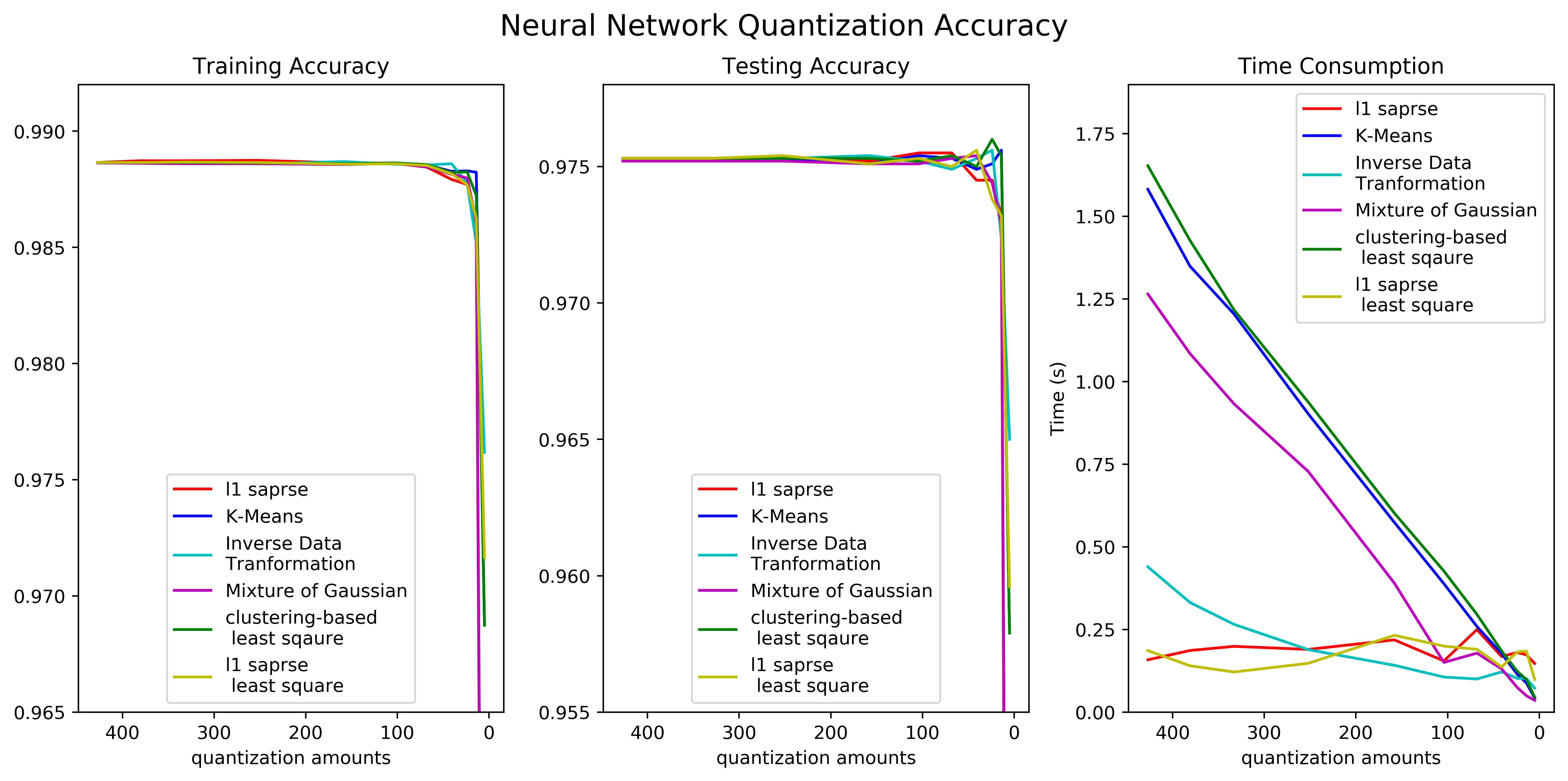

From the figures it can be found out that the proposed sparse regression-based methods can provide competitive performances for the last-layer quantization of the neural network. The pure sparse regression provides a slightly more deficient performance than other proposed methods, but in most cases the deficiency is negligible and it can still outperform Mixture of Gaussian-based quantization. Comparing to the time-consuming k-means based methods, the proposed methods can provide an alternative solution with much quicker running time. In addition, if the least square method is applied to optimize the of as algorithm 1 does, the algorithm will be able to provide no less competitive results than k-means method does in terms of accuracy, while the running time will remain at a low level. The clustering-based least square exact method can provide the overall optimal performance, especially in the area approaching to accuracy decrements. And the additional time consumed by solving least square on the top of k-means is negligible.
Figure 3 shows the values of the neural network last-layer quantization with different level of sparsity (quantization amounts). The full-column plot on the left is the weights solved by least square without sparsity. It could be found that even for the least square solution without any additional regularization term, some of the values of still hit the values around or equal to 0. The plots of the rest three columns represent the values of without least square, with least square and k-means based exact value methods, respectively. The trick behind the third plot is that the values of the dense vector are assigned to the starting index of each ’batch’ of same-values, which can form a equivalent illustration to a sparse parameter.
From the plots of -based quantization, it could be observed that almost all the are positive. This result is consistent with the characteristics of Coordinate Descent, which utilize a shrinkage operator and decreases small positive values to . The major difference between sparse least square methods and clustering-based method is that the latter tends to produce positive and negative values in roughly equivalent amounts. However, despite the differences between values of vectors, the two types of methods share a ’central zero area’ for index around 300-400. This implies that the proposed least square-based methods can capture the geometric information of the vector similar to clustering-based methods, while the time complexity is significantly lower. Furthermore, a most-positive vector is more consistent with the configuration of the matrix.

Moreover, to illustrate the effects of replacing with optimization, the performance of and optimization on the last-layer neural network data is illustrated in figure 4 with a coordinate descent optimization method implemented separately. Neither of the weights in the illustrated plots is optimized with least square. From the figure it could be observed that the method could in general lead to fewer quantization amounts for the same value, while produce a smaller loss comparing to the original. The experimental result also verifies the argument in section 3.3. However, despite the favorable performance, the algorithm could be sensitive to the value of , and it could be numerically very unstable if the value of is too large or too small. To improve the tolerance of in this algorithm could be a point of exploration in the future.

And finally, as for the quantization method, it could not find any non-trivial solution under the optimization method of [38], which indicated the drawbacks of numerical unreliability of -based method.
4.2 MNIST Image Quantization
Quantization could be used in image processing to reduce the number of values and space complexity. In this paper, a MNIST-digit image is chosen as an example to show the performance of image quantization of the proposed methods. The performances of two types of -based algorithms and two kinds of clustering-based methods are illustrated and compared in Fig.5. From the figure we could find out that K-means and the clustering-based least square optimization can provide the best performances in general, and there is no significant differences in terms of execution time. with least square optimization of values can provide less norm difference loss than using solely. Meanwhile, in terms of running time, the -based optimization approaches can provide significant advantages over K-means-based methods. Another remark of the MNIST quantization is that the K-means methods sometime provide out-of-range values (not in the interval ) when the number of clusters are large, and the reason can be attributed to bad initialization. However, for the least-square optimization methods, this problem does not happen at least in the MNIST circumstance.


The quantization result of method is shown separately in figure 6. It could be observed from the figure that the qualities of images are in general high and the loss is competitive. However, the problem of ’not universal’ is also very significant from the figures: in many cases, the algorithm could only find the largest possible quantization amounts smaller than the given value. In addition, the algorithm often fail to find solution when the required quantization amount is large.
4.3 Artificially-Generated Data with Specific Distributions
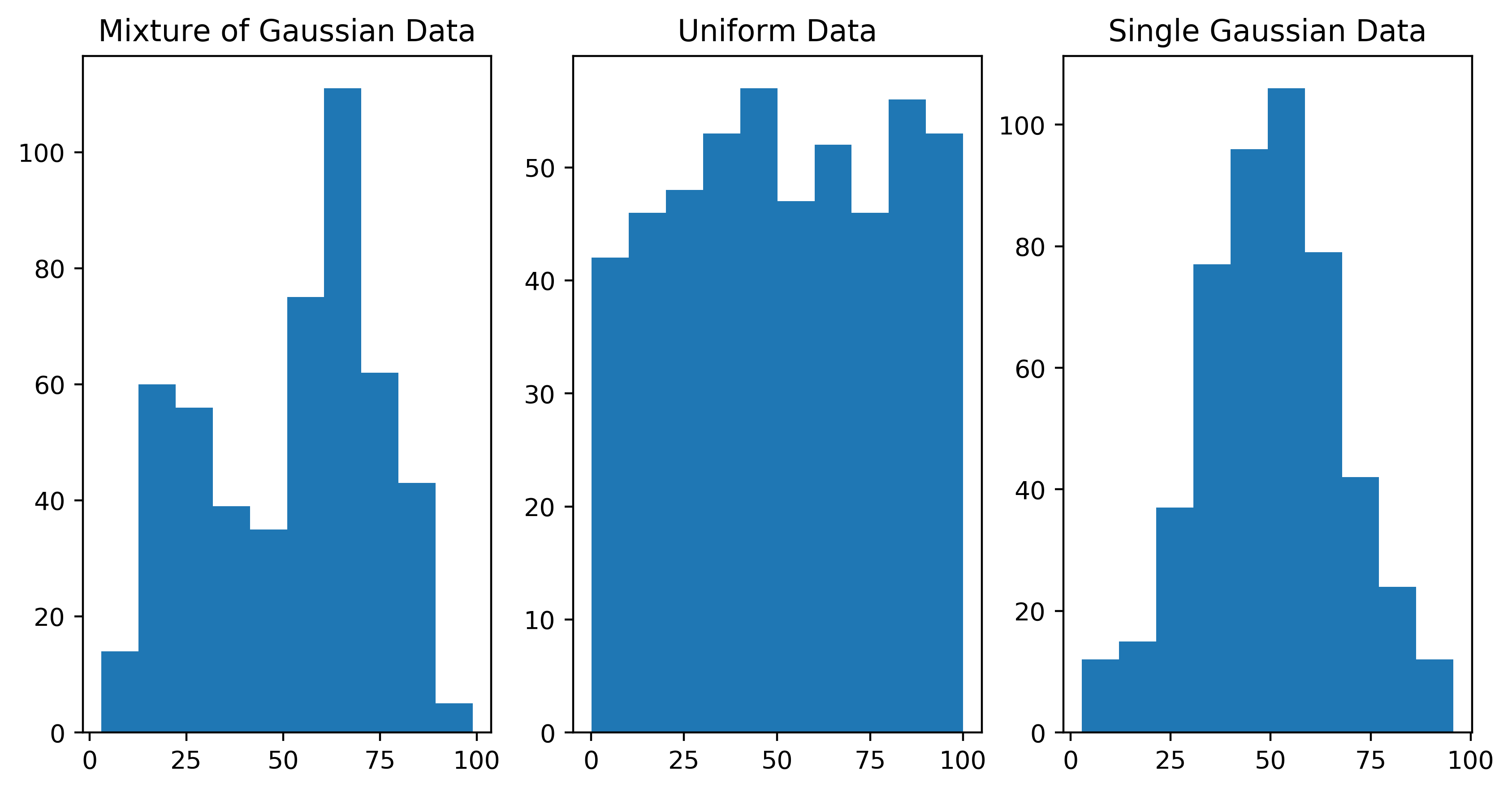
To test the performance of the proposed algorithms on data of different distributions, three types of distributions, namely Mixture of Gaussian, Uniform and Single Gaussian, are employed to generate 500 samples from each of them. The samples are constrained in the range of , and the distributions of the data we used could be shown as figure 7. In practice, these three types of distributions could describe most cases of 1-d data characteristics.
The experimental results for different quantization methods based on the above 3 types of data is shown in figure 8. From the figure, it could be observed that the information loss deficiency of without least square is more significant comparing to those for neural network and MNIST image. However, considering the running time reduced by the algorithm, the overall performance could still be regarded as merited. Also, if least square is employed to optimize the values of the vector, the information loss of approach will be only slightly higher than k-means based methods optimization, while the run-time will be still of great advantage comparing to the k-means branch of methods.

And finally, for the quantization method, again in the experiments it could not provide meaningful results for the quantization of the artificially-generated data. This problem further demonstrates the issue of using optimization despite its favourable information loss: getting the exact solution of is NP-hard, and with approximation optimization, there is a risk of failure in getting the results.
5 Conclusion
This paper proposed several sparse least square-based algorithms to better accomplish the task of scalar quantization. The characteristics and computational properties of the proposed algorithms are examined, and the advantages, drawbacks, and the advantageous scenarios of each of them are analyzed. The algorithms are implemented and tested under the scenarios of neural network weight, MNIST image and artificially-generated data respectively, and the results are demonstrated and analyzed. Experimental results shows that the proposed algorithms have competitive performances in terms of information loss/preservation, and the favorable properties in running time could make the -based algorithms especially useful when processing large batch of medium-size data and the number of post-quantization values are not far from the original.
The paper made the following major contributions: Firstly, it proposed several novel quantization methods with competitive information preservation ability and much more favorable time complexity; Secondly, the paper innovated the pioneering work of using least square optimization to solve the quantization problem, which could bring huge research potentials in the area; And thirdly, the algorithms proposed in the paper provide broader options for engineering practice, especially when the purpose of performing quantization is to restrict the number of distinct values to a high-resolution level, and when the number of post-quantization values is still large.
In the future, the authors intend to continue to explore quantization algorithms based on the idea initiated in the paper. One major problem of interests will be to extend the quantization method into high-dimensional vector scenarios by adopting novel target function and optimization method.
6 Acknowledgement
The authors would like to thank Mr. Feng Chen from Northwestern Polytechnical University, China, and Mr. Shixiong Wang from National University of Singapore, Singapore. Mr. Chen and Mr. Wang provided the authors many useful comments for the algorithms and programs of the research.
7 Declaration of interest
The authors declare no conflicts of interest.
References
- [1] P. C. Cosman, K. L. Oehler, E. A. Riskin, R. M. Gray, Using vector quantization for image processing, Proceedings of the IEEE 81 (1993) 1326–1341.
- [2] M. Saleem, Z. U. Rehman, U. Zahoor, A. Mazhar, M. R. Anjum, Self learning speech recognition model using vector quantization, in: 2016 Sixth International Conference on Innovative Computing Technology (INTECH), pp. 199–203.
- [3] H. Jegou, M. Douze, C. Schmid, Product quantization for nearest neighbor search, IEEE Transactions on Pattern Analysis and Machine Intelligence 33 (2011) 117–128.
- [4] K. F., A. E., D. G., Weight quantization for multi-layer perceptrons using soft weight sharing, Artificial Neural Networks (ICANN) 2130 (2001).
- [5] S. Han, H. Mao, W. J. Dally, Deep compression: Compressing deep neural network with pruning, trained quantization and huffman coding, CoRR abs/1510.00149 (2015).
- [6] V. Sze, Y. Chen, T. Yang, J. S. Emer, Efficient processing of deep neural networks: A tutorial and survey, CoRR abs/1703.09039 (2017).
- [7] Y. Gong, L. Liu, M. Yang, L. Bourdev, Compressing deep convolutional networks using vector quantization, arXiv preprint arXiv:1412.6115 (2014).
- [8] C. Wang, The Practical Implementation and Algorithm Exploration of Embedded Deep Learning (unpublished), Master’s thesis, Dept. of Computer Science, University College London, London, United Kingdom, 2017.
- [9] R. Azimi, M. Ghayekhloo, M. Ghofrani, H. Sajedi, A novel clustering algorithm based on data transformation approaches, Expert Systems with Applications 76 (2017) 59–70.
- [10] M. Elad, M. A. T. Figueiredo, Y. Ma, On the role of sparse and redundant representations in image processing, Proceedings of the IEEE 98 (2010) 972–982.
- [11] Z. Xiang, G. Joy, Color image quantization by agglomerative clustering, IEEE Computer Graphics and Applications (1994) 44–48.
- [12] S. Hsieh, K.-C. Fan, An adaptive clustering algorithm for color quantization, Pattern Recognition Letters 21 (2000) 337–346.
- [13] Q. Wen, M. E. Celebi, Hard versus fuzzy c-means clustering for color quantization, EURASIP Journal on Advances in Signal Processing 2011 (2011) 118.
- [14] H. L. Capitaine, C. Frélicot, A fast fuzzy c-means algorithm for color image segmentation, in: Proceedings of the 7th conference of the European Society for Fuzzy Logic and Technology, Atlantis Press, 2011/08, pp. 1074–1081.
- [15] S. Nowlan, G. Hinton, simplifying neural networks by soft weight-sharing, Neural Computation 4 (1992) 473–493.
- [16] K. Ullrich, E. Meeds, M. Welling, Soft Weight-Sharing for Neural Network Compression, ArXiv e-prints (2017).
- [17] T. Villmann, S. Haase, Divergence-based vector quantization, Neural Computation 23 (2011) 1343–1392. PMID: 21299418.
- [18] T. M. Martinetz, S. G. Berkovich, K. J. Schulten, ‘neural-gas’ network for vector quantization and its application to time-series prediction, IEEE Transactions on Neural Networks 4 (1993) 558–569.
- [19] B. Hammer, D. Hofmann, F.-M. Schleif, X. Zhu, Learning vector quantization for (dis-)similarities, Neurocomputing 131 (2014) 43 – 51.
- [20] P. T. Boufounos, Universal rate-efficient scalar quantization, IEEE transactions on information theory 58 (2012) 1861–1872.
- [21] W. Zhou, M. Yang, X. Wang, H. Li, Y. Lin, Q. Tian, Scalable feature matching by dual cascaded scalar quantization for image retrieval, IEEE transactions on pattern analysis and machine intelligence 38 (2016) 159–171.
- [22] L. Ai, J. Yu, Z. Wu, Y. He, T. Guan, Optimized residual vector quantization for efficient approximate nearest neighbor search, Multimedia Systems 23 (2017) 169–181.
- [23] E. C. Ozan, S. Kiranyaz, M. Gabbouj, Competitive quantization for approximate nearest neighbor search, IEEE Transactions on Knowledge & Data Engineering (2016) 1–1.
- [24] Y. Guo, A survey on methods and theories of quantized neural networks, arXiv preprint arXiv:1808.04752 (2018).
- [25] D. D. Lin, S. S. Talathi, V. S. Annapureddy, Fixed point quantization of deep convolutional networks, CoRR abs/1511.06393 (2015).
- [26] I. Hubara, M. Courbariaux, D. Soudry, R. El-Yaniv, Y. Bengio, Quantized neural networks: Training neural networks with low precision weights and activations., Journal of Machine Learning Research 18 (2017) 1–30.
- [27] E. Agustsson, F. Mentzer, M. Tschannen, L. Cavigelli, R. Timofte, L. Benini, L. V. Gool, Soft-to-hard vector quantization for end-to-end learning compressible representations, in: Advances in Neural Information Processing Systems, pp. 1141–1151.
- [28] M. A. Carreira-Perpinán, Y. Idelbayev, Model compression as constrained optimization, with application to neural nets. part ii: Quantization, arXiv preprint arXiv:1707.04319 (2017).
- [29] E. Candès, J. Romberg, Sparsity and incoherence in compressive sampling, Inverse Problems 23 (2007) 969–985.
- [30] J. Wright, Y. Ma, J. Mairal, G. Sapiro, T. S. Huang, S. Yan, Sparse representation for computer vision and pattern recognition, Proceedings of the IEEE 98 (2010) 1031–1044.
- [31] J. A. Tropp, A. C. Gilbert, Signal recovery from random measurements via orthogonal matching pursuit, IEEE Transactions on Information Theory 53 (2007) 4655–4666.
- [32] R. Tibshirani, Regression shrinkage and selection via the lasso: a retrospective, Journal of the Royal Statistical Society: Series B (Statistical Methodology) 73 (2011) 273–282.
- [33] J. Yang, Y. Zhang, Alternating direction algorithms for l1-problems in compressive sensing, SIAM Journal on Scientific Computing 33 (2011) 250–278.
- [34] F. Nie, H. Huang, X. Cai, C. H. Ding, Efficient and robust feature selection via joint l2,1-norms minimization, in: J. D. Lafferty, C. K. I. Williams, J. Shawe-Taylor, R. S. Zemel, A. Culotta (Eds.), Advances in Neural Information Processing Systems 23, Curran Associates, Inc., 2010, pp. 1813–1821.
- [35] M. Schmidt, G. Fung, R. Rosales, Fast optimization methods for l1 regularization: A comparative study and two new approaches, in: J. N. Kok, J. Koronacki, R. L. d. Mantaras, S. Matwin, D. Mladenič, A. Skowron (Eds.), Machine Learning: ECML 2007, Springer Berlin Heidelberg, Berlin, Heidelberg, 2007, pp. 286–297.
- [36] S. Gazagnes, E. Soubies, L. Blanc-Féraud, High density molecule localization for super-resolution microscopy using cel0 based sparse approximation, in: 2017 IEEE 14th International Symposium on Biomedical Imaging (ISBI 2017), pp. 28–31.
- [37] S. J. Wright, Coordinate Descent Algorithms, ArXiv e-prints (2015).
- [38] H. Hazimeh, R. Mazumder, Fast best subset selection: Coordinate descent and local combinatorial optimization algorithms, arXiv preprint arXiv:1803.01454 (2018).
- [39] F. Pedregosa, G. Varoquaux, A. Gramfort, V. Michel, B. Thirion, O. Grisel, M. Blondel, P. Prettenhofer, R. Weiss, V. Dubourg, J. Vanderplas, A. Passos, D. Cournapeau, M. Brucher, M. Perrot, E. Duchesnay, Scikit-learn: Machine learning in Python, Journal of Machine Learning Research 12 (2011) 2825–2830.
- [40] Z.-Q. Luo, P. Tseng, Error bounds and convergence analysis of feasible descent methods: a general approach, Annals of Operations Research 46 (1993) 157–178.
- [41] M. Hong, X. Wang, M. Razaviyayn, Z.-Q. Luo, Iteration complexity analysis of block coordinate descent methods, Mathematical Programming 163 (2017) 85–114.
- [42] H. Zou, T. Hastie, Regularization and variable selection via the elastic net, Journal of the Royal Statistical Society: Series B (Statistical Methodology) 67 (2005) 301–320.
- [43] E. Amaldi, V. Kann, On the approximability of minimizing nonzero variables or unsatisfied relations in linear systems, Theoretical Computer Science 209 (1998) 237 – 260.
- [44] P. Dhillon, Y. Lu, D. P. Foster, L. Ungar, New subsampling algorithms for fast least squares regression, in: Advances in neural information processing systems, pp. 360–368.