A novel approach for fusion of heterogeneous sources of data
Abstract
With advancements in sensor technology, heterogeneous sets of data such as those containing scalars, waveform signals, images, and even structured point clouds, are becoming increasingly popular. Developing statistical models based on such heterogeneous sets of data to represent the behavior of an underlying system can be used in the monitoring, control, and optimization of the system. Unfortunately, available methods only focus on the scalar and curve data and do not provide a general framework for integrating different sources of data to construct a model. This paper addresses the problem of estimating a process output, measured by a scalar, curve, image, or structured point cloud by a set of heterogeneous process variables such as scalar process setting, sensor readings, and images. We introduce a general multiple tensor-on-tensor regression (MTOT) approach in which each set of input data (predictor) and output measurements are represented by tensors. We formulate a linear regression model between the input and output tensors and estimate the parameters by minimizing a least square loss function. In order to avoid overfitting and reduce the number of parameters to be estimated, we decompose the model parameters using several bases that span the input and output spaces. Next, we learn the bases and their spanning coefficients when minimizing the loss function using a block coordinate descent algorithm combined with an alternating least square (ALS) algorithm. We show that such a minimization has a closed-form solution in each iteration and can be computed very efficiently. Through several simulation and case studies, we evaluate the performance of the proposed method. The results reveal the advantage of the proposed method over some benchmarks in the literature in terms of the mean square prediction error.
1 Introduction
With advancements in sensor technology, heterogeneous sets of data containing scalars, waveform signals, images, etc. are more and more available. For example, in semiconductor manufacturing, machine/process settings (scalar variables), sensor readings in chambers (waveform signals), and wafer shape measurements (images) may be collected to model and monitor the process. In this article, we refer to non-scalar variables as high-dimensional (HD) variables. Analysis and evaluation of such heterogeneous data sets can benefit many applications, including manufacturing processes (Szatvanyi et al.,, 2006; Wójcik & Kotyra,, 2009), food industries (Yu & MacGregor,, 2003), medical decision-making (Bellon et al.,, 1995), and structural health monitoring (Balageas et al.,, 2010). Specifically, analysis of such data may lead to the construction of a statistical model that estimates a variable (including HD) based on several other variables (regression model). Unfortunately, most works in regression modeling only consider scalars and waveform signals (Liang et al.,, 2003; Ramsay & Silverman,, 2005; Fan et al.,, 2014; Luo & Qi,, 2017), without including images or structured point clouds. However, in several applications, images or structured point clouds are available. For example, materials scientists are interested in constructing a link between process variables, e.g., the temperature and pressure under which a material is operating, and the microstructure of the material (Khosravani et al.,, 2017), which is often represented by an image or a variation of the microstructure image obtained by two-point statistics. Generating such a linkage model requires regression analysis between scalar and waveform process variables as inputs and an image. For more detailed information and a case study, please refer to (Gorgannejad et al.,, 2018).
As another example, in semiconductor manufacturing, overlay errors (defined as the difference between in-plane displacements of two layers of a wafer) are directly influenced by the shape of the wafer before the lithographic process. In this process, both the wafer shape and the overlay error (in the x and y directions) can be represented as images as shown in Figure 1. Prediction of the overlay error across a wafer based on the wafer shape can be fed forward to exposure tools for specific corrections (Turner et al.,, 2013). In order to predict the overlay error based on the wafer shape deformation, an image-on-image statistical model is required to capture the correlation between the wafer overlay and shape.


In addition to the space and computational issues caused by the large size of the HD variables, the challenge of developing an accurate model for a process with a heterogeneous group of variables is twofold: Integrating variables of different forms (e.g., scalars, images, curves) while capturing their “within” correlation structure. Mishandling this challenge can lead to an overfitted, inaccurate model. The regular regression approach that considers each observation within an HD variable as an independent predictor excessively increases the number of covariates in comparison to the sample size () and ignores the correlation between the observations. Consequently, this method may cause severe overfitting and produce inaccurate predictions. Principle component regression (PCR) alleviates the problem by first reducing the dimension of both the input variables and the output. Nevertheless, PCR fails to exploit the structure of images or point clouds. Furthermore, PCR determines the principle components (PCs) of the inputs and the outputs separately from each other without considering the interrelationship between them. Functional data analysis, specifically the functional regression model (FRM), has become popular in recent years due to its built-in data reduction functionality and its ability to capture nonlinear correlation structures (Liang et al.,, 2003; Ramsay & Silverman,, 2005; Yao et al.,, 2005; Fan et al.,, 2014; Ivanescu et al.,, 2015; Luo & Qi,, 2017). However, FRM requires a set of basis functions that is usually specified based on domain knowledge rather than a data-driven approach. Recently, Luo & Qi, (2017) proposed an approach that can combine several profiles and scalars to predict a curve, while learning the bases that span the input and output spaces. Nevertheless, it is not clear how to extend this approach to other forms of data effectively.
In the past few years, multilinear algebra (and, in particular, tensor analysis) has shown promising results in many applications from network analysis to process monitoring (Sun et al.,, 2006; Sapienza et al.,, 2015; Yan et al.,, 2015). Nevertheless, only a few works in the literature use tensor analysis for regression modeling. Zhou et al., (2013) has successfully employed tensor regression using PARAFAC/CANDECOMP (CP) decomposition to estimate a scalar variable based on an image input. The CP decomposition approximates a tensor as a sum of several rank-1 tensors (Kiers,, 2000). Zhou et al., (2013) further extended their approach to a generalized linear model for tensor regression in which the scalar output follows any exponential family distribution. Li et al., (2013) performed tensor regression with scalar output using Tucker decomposition. Tucker decomposition is a form of higher order PCA that decomposes a tensor into a core tensor multiplied by a matrix along each mode (Tucker,, 1963). CP decomposition is a special case of Tucker decomposition that assumes the same rank for all the basis matrices. Yan et al., (2017) performed the opposite regression and estimated point cloud data using a set of scalar process variables. Recently, Lock, (2017) developed a tensor-on-tensor regression (TOT) approach that can estimate a tensor using a tensor input while learning the decomposition bases. However, several limitations in TOT should be addressed. First, TOT uses CP decomposition, which restricts both the input and output bases to have exactly the same rank (say, ). This restriction may cause over- or under-estimation when the input and the output have different ranks. For example, when estimating an image based on few scalar inputs, the rank of the output can be far larger than the input matrix. Second and more importantly, this approach can only take into account a single tensor input and cannot be used effectively when multiple sources of input data with different dimensions and forms (e.g., a combination of scalar, curve, and image data) are available. The extension of TOT to multiple tensor inputs generates a significant challenge due to the first limitation previously mentioned. Because the output and the inputs should have the same rank, extending the TOT approach to multiple tensor inputs as well requires all the inputs to have the same rank (which is equal to the rank of the output). However, this means that in certain situations, such as when scalar and image inputs exist, one of the inputs should take the rank of the other, causing a severe underfitting or overfitting problem. One approach to allow multiple forms of data in TOT is to combine all the data into one single input tensor, e.g., an image and scalar input being merged by transforming each scalar value into a constant image. However, this approach generates a few issues: First, it significantly increases the size of the data, and second, it masks the separate effect of each input on the output due to the fusion of inputs. Furthermore, in situations in which the dimension of modes does not match (for example, a curve input with 60 observed points and an image of size 50x50), merging data into one tensor requires a method for dimension matching. Finally, the TOT approach fails to work on tensors of moderate size (e.g., on the image data of size 20000 pixels used in our case study) due to its high space complexity.
The overarching goal of this paper is to overcome the limitations of the previous methods, such as PCR, FRMs, and TOT, by constructing a unified regression framework that estimates a scalar, curve, image, or structured point cloud based on a heterogeneous set of (HD) input variables. This will be achieved by representing the output and each group of input variables as separate tensors and by developing a multiple tensor-on-tensor regression (MTOT). To avoid overfitting and estimating a large number of parameters, we perform Tucker decomposition on each group of inputs’ parameters using one set of bases to expand each of the input spaces and another set of bases to span the output space. We obtain the input bases by performing Tucker decomposition on the input tensors, then define a least square loss function to estimate the decomposition coefficients and output bases. To ensure uniqueness, we impose an orthonormality constraint over the output bases when minimizing the loss function and show a closed-form solution for both the bases and the decomposition coefficient in each iteration of our algorithm. This approach not only performs dimension reduction similar to PCR, but it also learns the output bases in accordance with the input space. Furthermore, the use of tensors to represent the data preserves the structure of an image or structured point cloud.
The rest of the article is organized as follows: In Section 2, we introduce notations and the multilinear algebra concepts used in the paper. In Section 3, we formulate the multiple tensor-on-tensor regression model and illustrate the closed-form solution for estimating the parameters. In Section 4, we describe four simulation studies. The first simulation study combines a profile and scalar data to estimate a profile output. This simulation study is particularly considered to compare MTOT to the available methods in functional regression. The second and third simulation studies contain images or point clouds either as the input or output. The fourth simulation considers estimating a nonsmooth profile using a set of scalar inputs. In each simulation study, we compare the performance of the proposed method with benchmarks in terms of (standardized) mean square prediction errors (MSPE). A case study on predicting the overlay errors based on the wafer shape is conducted in Section 5. Finally, we summarize the paper in Section 6.
2 Tensor Notation and Multilinear Algebra
In this section, we introduce the notations and basic tensor algebra used in this paper. Throughout the paper, we denote a scalar by a lower or upper case letter, e.g., or ; a vector by a boldface lowercase letter and a matrix by a boldface uppercase letter, e.g., and ; and a tensor by a calligraphic letter, e.g., . For example, we denote an order- tensor by , where is the dimension of the mode of tensor . We also denote a mode- matricization of tensor as , whose columns are the mode- fibers of the corresponding tensor , and . We also define a more general matricization of a tensor as follows: Let and be two sets that partition the set , which contains the dimensions of the modes of the tensor . Then, the matricized tensor is specified by , where and , and
where and . For simplicity of notation, we will denote as .
The Frobenius norm of a tensor can be defined as the Frobenius norm of any matricized tensor, e.g., . The mode- product of a tensor by a matrix is a tensor in and is defined as
The Tucker decomposition of a tensor decomposes the tensor into a core tensor and orthogonal matrices so that . The dimensions of the core tensor is smaller than , i.e., . Furthermore, the Kronecker product of two matrices and is denoted as and is obtained by multiplying each element of matrix to the entire matrix :
We link the tensor multiplication with the Kronecker product using the Proposition 1.
Proposition 1.
Let and , and let and , then
where is an unfold of the core tensor with and .
The proof of this proposition can be found in (Kolda,, 2006). Finally, the contraction product of two tensors and is denoted as and is defined as
3 Multiple Tensor-on-Tensor Regression Framework
In this section, we introduce the multiple tensor-on-tensor (MTOT) framework as an approach for integrating multiple sources of data with different dimensions and forms to model a process. Assume a set of training data of size is available and includes response tensors and input tensors , where is the number of inputs. The goal of MTOT is to model the relationship between the input tensors and the response using the linear form
| (1) |
where is the model parameter to be estimated and is an error tensor whose elements are from a random process. To achieve a more compact representation of the model (1), we can combine tensors , , and into one-mode larger tensors , , and and write
| (2) |
The matricization of (2) gives
| (3) |
where and are mode-1 unfolding of tensors and , respectively, and the first mode corresponds to the sample mode. is an unfold of tensor with and . It is intuitive that the parameters of (3) can be estimated by minimizing the mean squared loss function . However, this requires estimating parameters. For example, in the situation in which , minimizing the loss function gives a closed-form solution that requires estimating parameters. Estimating such a large number of parameters is prone to severe overfitting and is often intractable. In reality, due to the structured correlation between and , we can assume that the parameter lies in a much lower dimensional space and can be expanded using a set of basis matrices via a tensor product. That is, for each , we can write
| (4) |
where is a core tensor with and ; is a set of bases that spans the input space; and is a set of bases that spans the output space. With this low-dimensional representation, the estimation of reduces to learning the core tensor and the basis matrices and . In this paper, we allow to be learned directly from the input spaces. Two important choices of are truncated identity matrices (i.e., no transformation on the inputs) or the bases obtained from Tucker decomposition of the input tensor , i.e.,
In a special case that an input tensor is a matrix, the bases are the principle components (PCs) of that input if one uses Tucker decomposition. Allowing to be selected is reasonable because is an independent variable, and its basis matrices can be obtained separately from the output space. Furthermore, learning the core tensors and the bases provides a sufficient degree of freedom to learn . Next, we iteratively estimate the core tensors and the basis matrices by solving the following optimization problem:
| (5) |
where is a identity matrix. The first constraint ensures that the tensor of parameters is low-rank, and the orthogonality constraint ensures the uniqueness of both the bases and the core tensors when the problem is identifiable. In general, the problem of estimating functional data through a set of functions may not be identifiable under some conditions. That is, assuming , one can find , such that , i.e., and both estimate same mean value for the output. He et al., (2000); Chiou et al., (2004); Lock, (2017) discuss the identifiability problem in functional and tensor regression. Because the main purpose of this paper is to estimate and predict the output, we do not discuss the identifiability issue here, as learning any correct set of parameters will eventually lead to the same estimation of the output.
In order to solve (5), we combine the alternating least square (ALS) approach with the block coordinate decent (BCD) method (designated by ALS-BCD). The advantages of ALS algorithms that lead to their widespread use are conceptual simplicity, noise robustness, and computational efficiency (Sharan & Valiant,, 2017). In tensor decomposition and regression, due to the non-convex nature of the problem, finding the global optimum is often intractable, and it is well-known that the ALS algorithm also has no global convergence guarantee and may be trapped in a local optima (Kolda,, 2006; Sharan & Valiant,, 2017). However, ALS has shown great promise in the literature for solving tensor decomposition and regression applications with satisfying results. To be able to employ ALS-BCD, we first demonstrate Proposition 2:
Proposition 2.
When ,, and are known, a reshaped form of the core tensor can be estimated as
| (6) |
where and . Note that has fewer modes () than the original core tensor in (4), but it can be transformed into by a simple reshape operation.
The simplified proof of this proposition is given in Appendix A. Furthermore, if s are orthogonal, the core tensor can be obtained efficiently by the tensor product as
Note that in the situations in which sparsity of the core tensor is of interest, one can include a lasso penalty over the core tensor, and use numerical algorithms (e.g., Iterative Shrinkage-Thresholding Algorithm (Beck & Teboulle,, 2009)) to solve the problem. Furthermore, one can estimate the basis matrices as follows:
Proposition 3.
With known , , and , we can solve by
where and are obtained from the singular value decomposition of , where and ; and is the mode-i matricization of tensor . Note that is truncated.
The simplified proof of this proposition is shown in Appendix B. First note that we do not require calculation of the Kronecker product explicitly to find . In real implementation, we can use Proposition 1 to calculate the complete matrix using tensor products efficiently. Second, unlike the principle component regression (PCR) in which the principle components of the output are learned independent of the inputs, the estimated basis matrices directly depend on the input tensors, ensuring correlation between the bases and inputs. By combining Propositions 2 and 3, Algorithm 1 summarizes the estimation procedure for multiple tensor-on-tensor regression. This algorithm, in fact, combines the block coordinate decent (BCD) algorithm with the ALS algorithm.
3.1 Selection of tuning parameters
The proposed approach requires the selection of the values and . For simplicity and practicality, we assume that for each predictor and the response , the rank is fixed, i.e., and . As a result, we only need to select parameters. For this purpose, we use the k-fold cross-validation method on a -D grid of parameters and find the tuple of parameters that minimizes the mean squared error. As a result, we should define a grid over the rank values. This is achieved as following: First, we unfold each tensor and along their first mode. Next, we find the rank of each unfolded matrix, denoted as and . Then, for each and , we select the tuning parameters from and . Next, for each tuple , we calculate the average sum square error (RSS) and take the one that minimizes the RSS. For all studies in the next sections, we perform five-fold CV.
4 Performance Evaluation Using Simulation
This section contains two parts. In the first part, we only consider curve-on-curve regression and compare our proposed method to the function-on-function regression approach proposed by Luo & Qi, (2017), designated as sigComp. The reason we compare our approach to sigComp is that sigComp can handle multiple functional inputs (curves) and learn the basis functions similar to our approach. In the second part, we conduct a set of simulation studies to evaluate the performance of the proposed method when the inputs or outputs are in the form of images, structured point clouds, or curves with jumps. In this part, we compare the proposed method with two benchmarks: 1) The first benchmark is the TOT approach proposed by Lock, (2017), which can roughly be viewed as a general form of sigComp. Because this approach can only handle a single input tensor, when multiple inputs exist we perform a transformation to merge the inputs into one single tensor. 2) The second benchmark is based on principle component regression (PCR) similar to a benchmark considered in (Fan et al.,, 2014). In this approach, we first matricize all the input and output tensors, then perform principle component analysis to reduce the dimension of the problem by computing the PCA scores of the first few principle components that explain at least percent of the variation in the data. Next, we perform linear regression between the low-dimensional PC score of both inputs and output. More formally, let and denote the mode-1 matricization of the inputs and output, and be a concatenation of all the input matrices. We first compute the first and principle components of and the response . Next, the PC scores of the input are calculated (a matrix in ) and are used to predict the matrix of the scores of the response function (a matrix in ). Then, given the PC scores of the new inputs, we use the fitted regression model to predict the response scores. Finally, we multiply the predicted response scores by the principle components to obtain the original responses. The number of principle components and can be identified through a cross-validation procedure. In this paper, instead of cross-validating over and directly, we perform CV over the percentage of variation the PCs explain, i.e., . For this purpose, we take the value of from and take the that minimizes the CV error. The standardized mean square prediction error (SMSPE) is used as a performance measure to compare the proposed method with the benchmarks. The SMSPE is defined as
4.1 Simulation studies for curve-on-curve regression
In this simulation, we consider multiple functional (curve) predictors and multiple scalar predictors similar to the simulation study in (Luo & Qi,, 2017). We first randomly generate as follows:
where and are Gaussian processes with covariance function . Next, we generate functional predictors using the following procedure: Let be a matrix with the element equal to for and equal to one for diagonal elements. Next, we decompose , where is a matrix and generate a set of curves using a Gaussian process with covariance function . Finally, we generate the predictors at any given point as
With this formulation, each curve of is a Gaussian process with covariance function , and for each , the vector is a multivariate normal distribution with covariance . When , this vector becomes an independent vector of normally distributed variables. Figure 2 illustrates examples of the predictors when for . We also generate the scalar predictors from a multivariate normal distribution with mean vector zero and the covariance matrix with diagonal elements equal to and off-diagonal elements equal to . The coefficients of the scalar variables denoted by are generated from a Gaussian process with covariance function Finally, we generate the response curves as
where is generated from a normal distribution with zero mean and . We generate all of the input and output curves over and and take the samples over an equidistant grid of size .

For each combination of , we compare the performance of the proposed method with the methods in (Luo & Qi,, 2017) based on the mean square prediction error (MSPE) and the mean square estimation error (MSEE). We do not compare our approach to PCR in this simulation because sigComp has already demonstrated superiority over PCR in simulation studies in (Luo & Qi,, 2017). We implement the sigComp benchmark method using the R package FRegSigCom in which we use 50 spline bases for both the inputs and output and default convergence tolerance. To calculate the MSPE and MSEE, we first generate a sample data of size that is used to learn the model parameters. Next, we generate a testing sample of size and calculate MSPE as
and
We repeat this procedure 50 times to find the means and standard deviations of the MSPE and MSEE for each method. Table 1 reports the results at different values of and different numbers of predictors, . As reported, our proposed approach is superior to the sigComp method in terms of MSPE and MSEE for . For example, when and , the average MSPE and MSEE of the sigComp are and , which are much larger than the corresponding values ( and ) achieved by MTOT. However, the performance of sigComp is comparable or even slightly better than MTOT for . For example, when and , the average MSPE is for sigComp and for MTOT. The reason that sigComp performs slightly better for a larger is that it imposes sparsity when estimating the parameters, thus reducing the chance of overfitting. Figure 3 illustrates prediction examples obtained by each method, along with the true curve for different . As illustrated both of the approaches produce accurate predictions for .
| sigComp | MTOT | ||||
| MSPE | MSEE | MSPE | MSEE | ||
| 0 | 0.7155 (0.0413) | 0.6139 (0.0414) | 0.1039 (0.00130) | 0.0025 (0.0001) | |
| 0 | 0.2052 (0.0089) | 0.1048 (0.0087) | 0.1282 (0.0064) | 0.0286 (0.0061) | |
| 0.5 | 0.2086 (0.0105) | 0.0934 (0.0106) | 0.1159 (0.0034) | 0.0140 (0.0029) | |
| 0 | 0.1052 (0.0011) | 0.0055 (0.0011) | 0.1051 (0.0010) | 0.0053 (0.0003) | |
| 0.5 | 0.1104 (0.0018) | 0.0106 (0.008) | 0.1121 (0.0035) | 0.0141 (0.0043) | |

4.2 Simulation studies for image/ structured point-cloud or non-smooth output
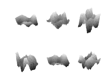
Case I–Waveform surface simulation: We simulate waveform surfaces based on two input tensors, and , where is the number of samples.
To generate the input tensors, we define . Then, we set , where Next, we randomly simulate elements of a core tensor from a standard normal distribution. Then, we generate an input sample using the following model: To generate a response tensor, we first simulate the elements of a core tensor from a standard normal distribution. Moreover, we set , where and . Next, we define the parameter tensors using the following expansion: Finally, we simulate a response tensor as where is the error tensor whose elements are sampled from a normal distribution . For simulation purposes, we assume , , and . That is, we generate a response based on a profile and an image signal. Furthermore, we set , , and . This implies that and . Figure 4a illustrates examples of generated response surfaces. For this simulation study, we first generate a set of data points. Then, we randomly divide the data into a set of size for training and a set of size for testing. We perform CV and train the model using the training set, then calculate the SMSPE for the proposed method and benchmarks based on the testing data. We repeat this procedure 50 times to capture the variance of the SMSPE. In order to prepare data for the TOT approach, three steps are performed: First, because the dimension of the curve inputs and the image inputs do not match, we randomly select points out of 60 to reduce the curve dimension to 50. Second, we replicate each curve 50 times to generate images. Third, for each sample, we merge the image constructed from the curve and the image input to construct a tensor of size . Combining all of the samples, we obtain an input tensor of size , where is the sample size.
Case II–Truncated cone simulation: We simulate a truncated cone based on a set of scalars and simple profile data in a 3D cylindrical coordinate system , where and . We first generate an equidistant grid of over the space by setting and . Specifically, we set . Next, we simulate the truncated cone over the grid by (7) where is the radii of the upper circle of the truncated cone, is the angle of the cone, is the eccentricity of the top and bottom surfaces, is the side curvatures of the truncated cone, and is process noise simulated from . Figure 4b illustrates examples of generated truncated cones. We assume that the parameters of the truncated cone are specific features obtained from a scalar and three simple profile data. In particular, we assume that the scalar predictor is and the profile predictors are , , and ; . That is, the inputs are one scalar and three profiles. We simulate these profiles for training purposes by setting the parameters as follows: We set , , , , and consider a full factorial design to generate samples. That is, for each combination of parameters (e.g., ), we generate a sample containing one scalar value and three profiles. We represent each of the inputs by a matrix (a tensor of order 2) to obtain four input matrices , , , and , where and . Finally, we generate the testing data by sampling the truncated cone parameters as follows: We assume , , , and , where denotes a uniform distribution over the interval , and sample each parameter from its corresponding distribution. In this simulation, we first train the model using the generated training data. Next, we generate a set of 1000 testing data. We predict the truncated cone based on the input values in the testing data and calculate the SMSPE for each predicted cone. In order to prepare the data for TOT, we first replicate the column of to generate a matrix of size , then merge this matrix with the other three matrices to construct an input tensor of size . This tensor is used as an input in the TOT.
Case III–Curve response with jump simulation: We
simulate a response function with jump using a group of B-spline bases.
Let with and and let
and
be two matrices of fourth-order B-spline bases obtained by one and
47 knots over . We generate a response profile
by combining these two bases as follows:
where and are
basis evaluations at the point , and
is a random error simulated from .
The input vector is dense, and its elements are generated
from a uniform distribution over . is
a sparse vector with five consecutive elements equal to one and the
rest equal to zero. The location of five consecutive elements is selected
at random. Figure 4c illustrates examples
of response functions. For this simulation study, we first generate
a set of data points, i.e., .
Then, we randomly divide the data into a set of size for training
and a set of size for testing. We perform CV and train the
model using the training data set. Next, we calculate the SMSPE for
the proposed method and the benchmark based on the testing data. We
repeat this procedure 50 times to capture the variance of the SMSPE.
In each case, we compare the proposed method with benchmarks based on the SMSPE calculated at different levels of noise . Tables 2, 3, and 4 report the average and standard deviation of SMSPE (or its logarithm), along with the average running time of each algorithm for the simulation cases I, II, and III, respectively. In Table 3, we report the average and standard deviation of the logarithm of the SMSPE for better comparison of the values. Please notice that the SMSPE is a standardized error and should not directly be compared to the variance. In all cases, the MTOT has the smallest prediction errors, reflecting the advantage of our method in terms of prediction. Furthermore, with the increase in , all methods illustrate a larger SMSPE in all cases. In the first case, the TOT illustrates a prediction performance comparable to our method at a cost of a much longer running time. For example, when , TOT requires about 147.33 seconds to reach the SMSPE of 0.0170, obtained in 1.05 seconds by MTOT. The performance of both PCR and TOT are significantly worse than MTOT in the second case. The inferior performance of TOT is due to both its restriction on selecting the same rank for both the input and output and the fact that the CP decomposition it uses does not consider the correlation between multiple modes.
In the third case, the prediction performances of all three methods are comparable, indicating that all three are capable of predicting a functional output with discontinuity. However, our approach shows slightly smaller prediction errors. Although the running time of the PCR is significantly lower than the other two approaches, MTOT running time is reasonable and within two-tenths of a second. The TOT shows slightly larger prediction error in all cases with much longer running time, making this approach less appealing. Recall that in this simulation, we used B-spline bases as the coefficients of the input to generate the output curve. Figure 5a illustrates the plot of the columns of the learned coefficient matrix that corresponds to . As can be seen, the learned bases are very similar to B-spline bases used originally as the coefficients. Figure 5b illustrates some of the columns of the learned parameters that correspond to . Unlike the first set of parameters, these parameters are slightly different from the B-spline bases that are originally used for data generation purposes. This is due to the identifiability issue. Our approach imposes an orthogonality restriction that may generate a set of parameters (when the identifiability issue exists) different from the parameters from which the data is originally generated, but that can still produce accurate predictions in terms of the mean value.

| PCR | TOT | MTOT | ||||
|---|---|---|---|---|---|---|
| SMSPE | Time (sec) | SMSPE | Time (sec) | SMSPE | Time (sec) | |
| 0.1 | 0.0057 (0.0015) | 0.03 (0.00) | 0.0046 (0.0011) | 154.98 (17.94) | 0.0044 (0.0011) | 1.05 (0.03) |
| 0.2 | 0.0199 (0.0045) | 0.04 (0.00) | 0.0170 (0.0039) | 147.33 (2.47) | 0.0170 (0.0040) | 1.05 (0.01) |
| 0.3 | 0.0455 (0.0097) | 0.04 (0.00) | 0.0399 (0.0086) | 149.03 (1.36) | 0.0395 (0.0086) | 1.05 (0.02) |
| 0.4 | 0.0773 (0.0233) | 0.04 (0.00) | 0.0678 (0.0135) | 149.13 (0.96) | 0.0673 (0.0212) | 1.05 (0.03) |
| 0.5 | 0.1186 (0.0222) | 0.04 (0.00) | 0.1036 (0.0231) | 146.17 (0.95) | 0.1032 (0.0203) | 1.04 (0.01) |
| 0.6 | 0.1670 (0.0327) | 0.04 (0.00) | 0.1456 (0.0309) | 147.75 (1.81) | 0.1454 (0.0299) | 1.03 (0.01) |
| PCR | TOT | MTOT | ||||
|---|---|---|---|---|---|---|
| log(SMSPE) | Time (sec) | log(SMSPE) | Time (sec) | log(SMSPE) | Time (sec) | |
| 0.01 | -5.555 (0.986) | 0.05 (0.00) | -5.249 (1.326) | 23.58 (5.93) | -8.095 (1.196) | 3.82 (0.09) |
| 0.02 | -5.509 (0.937) | 0.07 (0.00) | -5.197 (1.254) | 27.94 (6.11) | -7.629 (0.869) | 3.92 (0.10) |
| 0.03 | -5.441 (0.879) | 0.08 (0.00) | -5.127 (1.175) | 29.11 (8.46) | -7.215 (0.666) | 3.93 (0.12) |
| 0.04 | -5.360 (0.819) | 0.06 (0.00) | -5.048 (1.097) | 33.61 (9.02) | -6.856 (0.537) | 3.95 (0.14) |
| 0.05 | -5.269 (0.762) | 0.07 (0.00) | -4.963 (1.023) | 34.29 (14.55) | -6.543 (0.454) | 3.99 (0.13) |
| 0.06 | -5.173 (0.710) | 0.07 (0.00) | -4.875 (0.956) | 37.43 (15.19) | -6.266 (0.402) | 3.95 (0.14) |
| PCR | TOT | MTOT | ||||
|---|---|---|---|---|---|---|
| SMSPE | Time (sec) | SMSPE | Time (sec) | SMSPE | Time (sec) | |
| 0.1 | 0.0255 (0.0010) | 0.02 (0.00) | 0.0250 (0.0008) | 17.67 (0.58) | 0.0230 (0.0007) | 0.26 (0.01) |
| 0.15 | 0.0503 (0.0018) | 0.03 (0.00) | 0.0510 (0.0018) | 17.27 (0.20) | 0.0496 (0.0017) | 0.25 (0.01) |
| 0.2 | 0.0851 (0.0027) | 0.04 (0.00) | 0.0862 (0.0026) | 17.25 (0.22) | 0.0848 (0.0028) | 0.25 (0.01) |
| 0.25 | 0.1260 (0.0043) | 0.05 (0.00) | 0.1271 (0.0042) | 16.01 (2.32) | 0.1255 (0.0042) | 0.27 (0.00) |
| 0.3 | 0.1730 (0.0046) | 0.05 (0.00) | 0.1734 (0.0041) | 16.33 (2.67) | 0.1725 (0.0046) | 0.27 (0.01) |
| 0.35 | 0.2305 (0.0051) | 0.05 (0.00) | 0.2333 (0.0066) | 16.69 (0.83) | 0.2230 (0.0052) | 0.27 (0.00) |
5 Case Study
In semiconductor manufacturing, patterns are printed layer by layer over a wafer in a sequence of deposition, etching, and lithographic processes to manufacture transistors (Nishi & Doering,, 2000). Many of these processes induce stress variations across the wafer, distorting/changing the wafer shape (Brunner et al.,, 2013; Turner et al.,, 2013). Figure 6 illustrates a simplified sequence of processes, causing the overlay error in the patterned wafers. In the first step, a layer is deposited over the wafer and exposed to rapid thermal annealing, causing a curvature in the free-state wafer. The wafer is then chucked flat and patterned in a lithographic process. Next, to generate a second layer pattern, a new layer is deposited, changing the wafer shape. Finally, in the lithography step, the flattened wafer is patterned. Because the wafer is flattened, the first pattern distance increases, but the new pattern is printed with the same distance , generating a misalignment between patterns. The overlay error caused by lower order distortions can be corrected by most of the exposure tools. For this purpose, the alignment positions of several targets are measured and used to fit a linear overlay error model (Brunner et al.,, 2013):
| (8) |
where and identify the position of the target point over the wafer, and are transition errors, and relate to rotation error, and and are isotropic magnification errors pertaining to the wafer size change or wafer expansion due to processing. The fitted model is then used to correct the overlay errors. This model, however, can only correct the overlay error induced by a uniform stress field and fails to compensate for overlay errors caused by high-order distortions (Brunner et al.,, 2013). Therefore, developing a model that can relate the overlay error to higher order patterns in the wafer shape is essential for better overlay correction.

In this case study, we use our proposed method to predict the overlay error based on the wafer shape data. Such predictions can be fed forward to the exposure tools to result in a better correction strategy. In practice, the wafer shape is measured using a patterned wafer geometry (PWG) tool, and the overlay error is measured using standard optical methods (Brunner et al.,, 2013). Both the wafer shapes and the overlay errors (in each coordinate, x or y) can be presented as image data. In this case study, we follow the procedure and results suggested and verified (through both experiments and finite element [FE] analysis) by Brunner et al., (2013) to generate surrogate data of overlay errors based on the wafer shape prior to two lithography steps (, ). The data generation procedure is elaborated in Appendix C.
Based on the described procedure in Appendix C, we generate a set of 500 training observations, i.e., wafer shapes and overlay errors, , and employ our proposed method to estimate the based on . Because in our simulated data remains fixed, we consider as the predictor. We also generate 100 observations as the test dataset. The mean square prediction error obtained from the testing data is used as the performance criterion. We repeat the simulations 50 times and record the MSPE values. Because our proposed methodology assumes that the shapes are observed over a grid, we transform the data to the polar coordinate prior to modeling. In the polar space, each shape is observed over a grid of ( in the radial direction and in the angular direction, with overall 20,000 pixels). Unfortunately, the TOT approach proposed by Lock, (2017) failed to run with this size of images due to its high space complexity. Therefore, we only compared our approach with PCR. Figure 7 illustrates an example of the original and predicted corrected overlay error image, along with the prediction error. As illustrated, the proposed method predicted the original surface more accurately, with smaller errors across the wafer. Figure 8 illustrates the boxplots of the logarithm of the prediction mean square error calculated over the 50 replications in contrast with the benchmark. The results show that the proposed method is superior to the benchmark in prediction of the image. As an example, the average of log(SMSE) over the replications is -8.33 for the proposed method and -7.56 for the PCR approach.


6 Conclusion
This paper proposed a multiple tensor-on-tensor approach for modeling processes with a heterogeneous set of input variables and an output that can be measured by a scalar, curve, image, or point-cloud, etc. The proposed method represents each of the inputs as well as the output by tensors, and formulates a multiple linear regression model over these tensors. In order to estimate the parameters, a least square loss function is defined. In order to avoid overfitting, the proposed method decomposes the regression parameters through a set of basis matrices that spans the input and output spaces. Next, the basis matrices, along with their expansion coefficients, are learned by minimizing the loss function. The orthogonality condition is imposed over the output bases to assure identifiability and interpretability. To solve the minimization problem, first, a closed-form solution is derived for both the bases and their coefficients. Second, the block coordinate decent (BCD) approach combined with the ALS algorithm is applied. The proposed approach is capable of combining different forms of inputs (e.g., an image, a curve, and a scalar) to estimate an output (e.g., a scalar, a curve, or an image, etc.) as demonstrated in first three simulation studies. For example, in the first and third simulation studies, we combined the scalar and profile inputs to estimate a profile and a point cloud, respectively; and in the second simulation study, a profile and an image are integrated to predict an image.
In order to evaluate the performance of the proposed method, we conducted four simulation studies and a case study. In our first simulation study, we compared our proposed method with the function-on-function approach proposed by Luo & Qi, (2017). This simulation considered scalar and curve inputs since the benchmark can only handle those form of data. Next, we performed three other simulations to evaluate the performance of the proposed method when the inputs or outputs are images or point clouds. In these simulation studies, the proposed approach was compared with principle component regression (PCR) and tensor-on-tensor (TOT) regression, and showed superior performance in terms of mean squared prediction error. We also evaluated our proposed method using a set of surrogate data generated according to the manufacturing process of semiconductors. We simulated the shape and overlay errors for several wafers and applied the proposed method to estimate the overlay errors based on the wafer shapes measured prior to the lithography steps. Results showed that the proposed method performed significantly better than the PCR in predicting the overlay errors.
As a future work, including penalties such as lasso for sparsity and group lasso for variable selection and imposing roughness penalties over the basis matrices may improve the prediction results and can be further studied.
Appendix A: Proof of Proposition 2
For simplicity, we assume only one input tensor exists. Then, we can solve by
Appendix B: Proof of Proposition 3
Again assuming a single input tensor, let us define in the tensor format as , which can be written as . First note that
with . Then, we want to solve
This is an orthogonal procrustes problem and is known to have solution as is stated in Proposition 3.
Appendix C: Simulating the Overlay Error
Brunner et al., (2013) introduced a measure based on in-plane distortion (IPD) called predicted in-plane distortion residual (PIR) to estimate and predict nonuniform-stress-induced overlay errors based on wafer shape. For this purpose, they first illustrate that the IPD is proportional to gradient of wafer shape , i.e.,
Then, for two layers, say and , to be patterned, they calculate the IPD and subtract them to find the shape-slope difference, i.e., . The shape-slope is then corrected based on model (8) to find the shape-slope residual (SSR). Finally, Brunner et al., (2013) calculated the PIR as a factor of SSR. That is,
where is a constant that depends on the wafer thickness. In their study, they showed through four differently patterned engineer stress monitor (ESM) wafers that the PIR is linearly correlated by the overlay errors with high values (e.g., 92%). To perform the experiment, they first deposit a layer of silicon nitride film over a 300mm wafer as a source of stress. This process changes the wafer shape and causes the wafer to curve. The shape of the wafer is measured by a patterned wafer geometry (PWG) tool designed for the metrology of 300mm wafers. After the wafer is exposed by a designed pattern (four different patterns considered in this study), it goes through an etching process that relieves some part of the stress depending on the pattern density. At this stage, and prior to next lithography step, the wafer shape is again measured. After the second lithography step, the overlay error is measured using standard optical methods. Using the measured wafer shapes, they calculated the PIR and showed a high correlation between the PIR and overlay error.
In our study, we first simulate the wafer shapes and then estimate the overlay errors using the following procedure introduced by Brunner et al., (2013). Simulating a wafer shape requires knowledge of the different components in wafer geometry. Brunner et al., (2013) and Turner et al., (2013) consider several wafer shape features that span different ranges of spatial wavelength . At the highest level is the overall shape of the wafer represented by a bow (or warp) in the range of tens of micrometers. Other shape variations are those that are spanned by spatial wavelengths in the range of several meters and waveheight in the micrometer range. Another component is the nanotopography (NT) of the wafer, with ranging from few millimeters to 20mm and the wave-height in nanometers. Finally, the roughness of the wafer is defined as variations with mm. In this study, we only consider the bow shape and the NT components when simulating a wafer shape. The wafer shapes are simulated as follows: We first assume that a thin layer is deposited over a wafer, which causes only a bow shape geometry in the wafer (that is, we assume no wave patterns). We simulate the bowed wafer geometry using , where is the warp or bow size and is assumed to be , and is the wafer radius, which is assumed to be mm. We then assume that a lithography/etching process is performed and the wafer shape changes in both bow and wavy patterns as follows:
where is the bow size uniformly sampled from to , and and are the waveheight and wavelength, respectively. Moreover, is the number of waveforms assumed. For each wafer (i.e. sample), we first randomly select from and then select wavelength from for NT wavelength. Finally, we sample waveheight from to ensure that the large wavelength has large a waveheight and vice versa. After simulating a wafer shape prior to two lithography steps, we calculate the IPD and PIR according to the procedure described previously. Note that we only calculate the values proportional to the original values. Figure 9 illustrates an example of generated shapes, their associated IPDs in the x coordinates, i.e., , and the difference between the x coordinate IPDs prior to and after correction. In order to correct the IPD values, we consider a second order model:
which is fitted to the calculated values of and . Then the fitted model is subtracted from the and to find the corrected values. The corrected values are associated with the PIR and the overlay error.

References
- Balageas et al., (2010) Balageas, Daniel, Fritzen, Claus-Peter, & Güemes, Alfredo. 2010. Structural Health Monitoring. Vol. 90. John Wiley & Sons.
- Beck & Teboulle, (2009) Beck, Amir, & Teboulle, Marc. 2009. A fast iterative shrinkage-thresholding algorithm for linear inverse problems. SIAM Journal on Imaging Sciences, 2(1), 183–202.
- Bellon et al., (1995) Bellon, E, Van Cleynenbreugel, J, Delaere, D, Houtput, W, Smet, M, Marchal, G, & Suetens, P. 1995. Experimental teleradiology. novel telematics services using image processing, hypermedia and remote cooperation to improve image-based medical decision making. Journal of Telemedicine and Telecare, 1(2), 100–110.
- Brunner et al., (2013) Brunner, Timothy A, Menon, Vinayan C, Wong, Cheuk Wun, Gluschenkov, Oleg, Belyansky, Michael P, Felix, Nelson M, Ausschnitt, Christopher P, Vukkadala, Pradeep, Veeraraghavan, Sathish, & Sinha, Jaydeep K. 2013. Characterization of wafer geometry and overlay error on silicon wafers with nonuniform stress. Journal of Micro/Nanolithography, MEMS, and MOEMS, 12(4), 043002–043002.
- Chiou et al., (2004) Chiou, Jeng-Min, Müller, Hans-Georg, & Wang, Jane-Ling. 2004. Functional response models. Statistica Sinica, 675–693.
- Fan et al., (2014) Fan, Yingying, Foutz, Natasha, James, Gareth M, Jank, Wolfgang, et al. 2014. Functional response additive model estimation with online virtual stock markets. The Annals of Applied Statistics, 8(4), 2435–2460.
- Gorgannejad et al., (2018) Gorgannejad, Sanam, Reisi Gahrooei, Mostafa, Paynabar, Kamran, & Neu, Richard W. 2018. Characterizing the aged state of Ni-based superalloys based on process variables using PCA and tensor regression. Acta Materialia, submitted.
- He et al., (2000) He, G, Müller, HG, & Wang, JL. 2000. Extending correlation and regression from multivariate to functional data. Asymptotics in Statistics and Probability, 197–210.
- Ivanescu et al., (2015) Ivanescu, Andrada E, Staicu, Ana-Maria, Scheipl, Fabian, & Greven, Sonja. 2015. Penalized function-on-function regression. Computational Statistics, 30(2), 539–568.
- Khosravani et al., (2017) Khosravani, Ali, Cecen, Ahmet, & Kalidindi, Surya R. 2017. Development of high throughput assays for establishing process-structure-property linkages in multiphase polycrystalline metals: Application to dual-phase steels. Acta Materialia, 123, 55–69.
- Kiers, (2000) Kiers, Henk AL. 2000. Towards a standardized notation and terminology in multiway analysis. Journal of Chemometrics, 14(3), 105–122.
- Kolda, (2006) Kolda, Tamara Gibson. 2006. Multilinear operators for higher-order decompositions. Tech. rept. Sandia National Laboratories.
- Li et al., (2013) Li, Xiaoshan, Zhou, Hua, & Li, Lexin. 2013. Tucker tensor regression and neuroimaging analysis. arxiv preprint arxiv:1304.5637.
- Liang et al., (2003) Liang, Hua, Wu, Hulin, & Carroll, Raymond J. 2003. The relationship between virologic and immunologic responses in AIDS clinical research using mixed-effects varying-coefficient models with measurement error. Biostatistics, 4(2), 297–312.
- Lock, (2017) Lock, Eric F. 2017. Tensor-on-tensor regression. arxiv preprint arxiv:1701.01037.
- Luo & Qi, (2017) Luo, Ruiyan, & Qi, Xin. 2017. Function-on-function linear regression by signal compression. Journal of the American Statistical Association, 1–16.
- Nishi & Doering, (2000) Nishi, Yoshio, & Doering, Robert. 2000. Handbook of Semiconductor Manufacturing Technology. CRC Press.
- Ramsay & Silverman, (2005) Ramsay, James, & Silverman, BW. 2005. Functional Data Analysis. Springer Science & Business Media.
- Sapienza et al., (2015) Sapienza, Anna, Panisson, André, Wu, Joseph, Gauvin, Laetitia, & Cattuto, Ciro. 2015. Detecting anomalies in time-varying networks using tensor decomposition. Pages 516–523 of: IEEE International Conference on data Mining Workshop (ICDMW).
- Sharan & Valiant, (2017) Sharan, Vatsal, & Valiant, Gregory. 2017. Orthogonalized ALS: A theoretically principled tensor decomposition algorithm for practical use. arxiv preprint arxiv:1703.01804.
- Sun et al., (2006) Sun, Jimeng, Papadimitriou, Spiros, & Philip, S Yu. 2006. Window-based tensor analysis on high-dimensional and multi-aspect streams. Pages 1076–1080 of: ICDM.
- Szatvanyi et al., (2006) Szatvanyi, G, Duchesne, C, & Bartolacci, G. 2006. Multivariate image analysis of flames for product quality and combustion control in rotary kilns. Industrial & Engineering Chemistry Research, 45(13), 4706–4715.
- Tucker, (1963) Tucker, Ledyard R. 1963. Implications of factor analysis of three-way matrices for measurement of change. Problems in Measuring Change, 122137.
- Turner et al., (2013) Turner, Kevin T, Ramkhalawon, Roshita, & Sinha, Jaydeep K. 2013. Role of wafer geometry in wafer chucking. Journal of Micro/Nanolithography, MEMS, and MOEMS, 12(2), 023007–023007.
- Wójcik & Kotyra, (2009) Wójcik, Waldemar, & Kotyra, Andrzej. 2009. Combustion diagnosis by image processing. Photonics Letters of Poland, 1(1), 40–42.
- Yan et al., (2015) Yan, Hao, Paynabar, Kamran, & Shi, Jianjun. 2015. Image-based process monitoring using low-rank tensor decomposition. IEEE Transactions on Automation Science and Engineering, 12(1), 216–227.
- Yan et al., (2017) Yan, Hao, Paynabar, Kamran, & Pacella, Massimo. 2017. Structured point cloud data analysis for process modeling and optimization. Technometrics, submitted.
- Yao et al., (2005) Yao, Fang, Müller, Hans-Georg, Wang, Jane-Ling, et al. 2005. Functional linear regression analysis for longitudinal data. The Annals of Statistics, 33(6), 2873–2903.
- Yu & MacGregor, (2003) Yu, Honglu, & MacGregor, John F. 2003. Multivariate image analysis and regression for prediction of coating content and distribution in the production of snack foods. Chemometrics and Intelligent Laboratory Systems, 67(2), 125–144.
- Zhou et al., (2013) Zhou, Hua, Li, Lexin, & Zhu, Hongtu. 2013. Tensor regression with applications in neuroimaging data analysis. Journal of the American Statistical Association, 108(502), 540–552.