Redundancy Allocation in Finite-Length Nested Codes for Nonvolatile Memories

The BDC in Fig. 1 can be described as follows. Let “$\circ$” denote the operator $\circ:\{0,1\}\times\left\{0,1,\lambda\right\}\rightarrow\{0,1\}$ as in [18]

By using the operator $\circ$, an $n$-cell memory with stuck-at defects is modeled by

where ${\mathbf{c}},{\mathbf{y}}\in\left\{0,1\right\}^{n}$ are the codeword and the channel output vector, respectively. Also, the channel state vector ${\mathbf{s}}\in\left\{0,1,\lambda\right\}^{n}$ represents the defect information in the $n$-cell memory. Note that $\circ$ is the vector component-wise operator.

As shown in Fig. 1, the probabilities of stuck-at defects and normal cells are given by

Now we consider the channel models with both permanent stuck-at defects and transient errors, i.e., the BDEC and the BDSC. For the BDEC, $\mathbf{c}\circ\mathbf{s}$ will be the channel input of the BEC with the erasure probability $\alpha$. Also, the BDSC can be modeled by

where $\mathbf{c}\circ\mathbf{s}$ is the channel input of the binary symmetric channel (BSC) with the crossover probability $p$ and ${\mathbf{z}}\in\{0,1\}^{n}$ is the random error vector.

Assuming that stuck-at defects do not suffer from transient errors, the capacity can be determined by the following theorem.

where $\widetilde{C}$ is the capacity of the discrete memoryless channel (DMC) with $P(Y\mid X)=P(Y\mid X,S=\lambda)$. The superscript ‘max’ in (7) represents the capacity when the defect information is fully known to both the encoder and decoder. Also, the superscript ‘enc’ denotes the capacity when only the encoder knows the defect information. Since $\widetilde{C}^{\text{enc}}$ is the same as $\widetilde{C}^{\text{max}}$, we can omit the superscript if the stuck-at defects do not suffer from transient errors.

Let $\widetilde{C}_{\text{BDEC}}$ denote the capacity of the channel when only the normal cells can be erased. Similarly, let $\widetilde{C}_{\text{BDSC}}$ denote the capacity of the channel when only the normal cells suffer from random errors. By Theorem 1, it is clear that

where $h\left(x\right)=-x\log_{2}x-\left(1-x\right)\log_{2}\left(1-x\right)$. If neither the encoder nor the decoder knows the defect information, the capacity is given by [3]

which is the capacity of the BSC with the crossover probability

If both the stuck-at defects and the normal cells suffer from transient errors, it is difficult to derive closed-from expressions for $C_{\text{BDSC}}^{\text{max}}$ and $C_{\text{BDSC}}^{\text{enc}}$. Note that the superscript ‘max’ represents the capacity when the defect information is fully known to both the encoder and decoder and the superscript ‘enc’ represents the capacity when only the encoder knows the defect information. Instead, these capacities can be evaluated numerically [3]. For the BDEC, we can derive $C_{\text{BDEC}}^{\text{max}}$ and $C_{\text{BDEC}}^{\text{enc}}$ because of the channel model’s simpleness. If both the encoder and decoder know the defect information, this channel is equivalent to the BEC with the erasure probability of $\alpha+\beta-\alpha\beta$. Hence,

which is the same as in (8). The capacity $C_{\text{BDEC}}^{\text{enc}}$ is derived as follows.

Although $C_{\text{BDEC}}^{\text{enc}}<C_{\text{BDEC}}^{\text{max}}=\widetilde{C}_{\text{BDEC}}$, the difference between $C_{\text{BDEC}}^{\text{enc}}$ and $\widetilde{C}_{\text{BDEC}}$ is only $\alpha\beta$ which is much smaller than $\alpha$ or $\beta$ for $\alpha,\beta\ll 1$.

For the BDSC, the closed-form expressions for $C_{\text{BDSC}}^{\text{max}}$ and $C_{\text{BDSC}}^{\text{enc}}$ are not known. In [18], only a non-closed-form expression for $C_{\text{BDSC}}^{\text{enc}}$ was derived. Although we cannot obtain a closed-form expression for $C_{\text{BDSC}}$, we derive the following bound.

From (15) and (16), we can see that the difference between the upper bound and lower bound is only $\beta h(p)$. For $\beta,p\ll 1$, $\beta h(p)$ is much smaller than $\beta$ and $h(p)$.

In [18], Heegard proposed the PLBCs which can be viewed as nested codes [19]. PLBCs are capable of correcting both stuck-at errors (due to stuck-at defects) and transient errors. Note that the PLBC can correct transient errors occurring in both stuck-at defects and normal cells. An $[n,k,l]$ PLBC is a pair of linear subspaces ${\mathcal{C}}_{1}\subset\{0,1\}^{n}$ and ${\mathcal{C}}_{0}\subset\{0,1\}^{n}$ of dimension $k$ and $l$ such that ${\mathcal{C}}_{1}\cap{\mathcal{C}}_{0}=\{\mathbf{0}\}$. Then the direct sum

is an $[n,k+l]$ linear block code with a generator matrix $\widetilde{G}=\left[G_{1}\quad G_{0}\right]$. Note that the sizes of $G_{1}$ and $G_{0}$ are $n\times k$ and $n\times l$, respectively. An example of PLBC can be found in [18].

The encoding and decoding are described as follows. Encoding: A message $\mathbf{m}$ is encoded to a corresponding codeword $\mathbf{c}=\mathbf{c}_{1}+\mathbf{c}_{0}=G_{1}\mathbf{m}+G_{0}\mathbf{d}$. First, we encode $\mathbf{m}$ into $G_{1}\mathbf{m}$ for correcting transient errors. Next, the stuck-at defects are masked by $G_{0}\mathbf{d}$ where $\mathbf{d}$ is chosen carefully to mask stuck-at defects.

Decoding: Let the received vector be $\mathbf{y}=\mathbf{c}\circ\mathbf{s}+\mathbf{z}$ according to (6). The decoder computes the syndrome ${\mathbf{v}}=\widetilde{H}^{T}{\mathbf{y}}$ (superscript $T$ denotes transpose) where $\widetilde{H}$ is the parity check matrix of $\mathcal{C}$ such that $\widetilde{H}^{T}\widetilde{G}=0_{r,k+l}$ (the $r\times(k+l)$ all-zero matrix). Based on the syndrome $\mathbf{v}$, the decoder chooses $\widehat{\mathbf{z}}$ (i.e., the estimate of $\mathbf{z}$) such that $\widetilde{H}^{T}\widehat{\mathbf{z}}=\mathbf{v}$. Then $\widehat{\mathbf{m}}=\widetilde{G}_{1}^{T}\widehat{\mathbf{c}}$ where $\widehat{\mathbf{c}}=\mathbf{y}+\widehat{\mathbf{z}}$. The message inverse matrix $\widetilde{G}̃_{1}$ is defined as an $n\times k$ matrix such that $\widetilde{G}̃_{1}^{T}G_{1}=I_{k}$ and $\widetilde{G}̃_{1}^{T}G_{0}=0_{k,l}$.

Note that $d_{1}$ is greater than or equal to the minimum distance of the $[n,k+l]$ linear block code with the parity check matrix $\widetilde{H}$, while $d_{0}$ is the minimum distance of the $[n,k+r]$ linear block code with the parity check matrix $G_{0}$ [18].

It is critical to choose the proper $\mathbf{d}$ during the encoding stage of PLBC. The minimum distance encoding (MDE) chooses $\mathbf{d}$ as follows.

where $\|{\mathbf{c}}\circ{\mathbf{s}}-{\mathbf{c}}\|$ represents the number of errors due to stuck-at defects and ${\mathbf{b}}=G_{1}{\mathbf{m}}+{\mathbf{s}}$. Also, ${\mathcal{U}}=\left\{i_{1},\ldots,i_{u}\right\}$ indicates the set of locations of stuck-at defects. We use the notation of ${\mathbf{s}}^{\mathcal{U}}=\left(s_{i_{1}},\ldots,s_{i_{u}}\right)^{T}$, $G_{0}^{\mathcal{U}}=\left[{\mathbf{g}}_{0,i_{1}}^{T},\ldots,{\mathbf{g}}_{0,i_{u}}^{T}\right]^{T}$, and $G_{1}^{\mathcal{U}}=\left[{\mathbf{g}}_{1,i_{1}}^{T},\ldots,{\mathbf{g}}_{1,i_{u}}^{T}\right]^{T}$ where ${\mathbf{g}}_{0,i}$ and ${\mathbf{g}}_{1,i}$ are the $i$-th rows of $G_{0}$ and $G_{1}$ respectively.

By solving the optimization problem in (19), we can minimize the number of errors due to stuck-at defects. It was shown [18] that the capacity of the BDSC can be achieved by the MDE and the maximum likelihood decoding (MLD). However, the encoding complexity of the MDE is ${\mathcal{O}}(2^{u})$. Instead of solving the exponential complexity optimization problem, we just try to solve the following linear equation.

Gaussian elimination or some other linear equation solution methods can be used to solve (20) with ${\mathcal{O}}\left(u^{3}\right)$ complexity. If the encoder fails to find a solution of (20), then encoding failure is declared. It is clear that (20) has at least one solution if and only if

where $\left(G_{0}^{\mathcal{U}}\mid\mathbf{b}^{\mathcal{U}}\right)$ denotes the augmented matrix. If $u<d_{0}$, $\rank\left(G_{0}^{\mathcal{U}}\right)$ is always $u$ by (18). Hence, (21) holds and at least one solution $\mathbf{d}$ exists. If $u\geq d_{0}$, the encoder may fail to find a solution of (20).

For convenience, we define a random variable $E$ as follows.

We observe that the probability of encoding failure $P(E=0)$ by solving (19) is the same as $P(E=0)$ by solving (20). It is because $G_{0}^{\mathcal{U}}\mathbf{d}\neq\mathbf{b}^{\mathcal{U}}$ if and only if $\|{\mathbf{c}}\circ{\mathbf{s}}-{\mathbf{c}}\|\neq 0$. Although solving (20) is suboptimal in regards to the number of stuck-at errors (i.e., $\|{\mathbf{c}}\circ{\mathbf{s}}-{\mathbf{c}}\|$), $C_{\text{BDC}}$ can be achieved by solving (20) instead of (19), which is shown in the following Proposition by using the results of [18].

We note that Dumer proposed an asymptotically optimal code for the BDC with encoding complexity ${\mathcal{O}}\left(n\log_{2}^{3}{n}\right)$ [5]. In this paper, we are focusing on Heegard’s partitioned codes with encoding by solving linear equation of (20). It is because this linear equation approach allows to derive the upper bound on encoding failure probability based on linear algebra. This upper bound plays a pivotal role in estimating the optimal redundancy allocation for the BDEC and the BDSC. Moreover, for a finite-length $n$ and a reasonable defect probability $\beta$, $u\simeq\beta n$ is not a large number, hence, the computational complexity ${\mathcal{O}}(u^{3})$ is not high.

Since we focus on the redundancy allocation problem in finite-length codes, we derive an upper bound on $P(E=0)$ for finite $n$. During the encoding stage, $\mathbf{d}$ is chosen by solving the linear equation (20) instead of the optimization problem (19).

Lemma 3.9 supports that $P\left(E=0\mid U=u\right)=0$ for $u<d_{0}$. The following Lemma states that $P\left(E=0\mid U=u\right)$ can be obtained exactly for $d_{0}\leq u\leq d_{0}+\left\lfloor\frac{d_{0}-1}{2}\right\rfloor$ where $\lfloor x\rfloor$ is the largest integer not greater than $x$.

From the definition of $d_{0}$ in (18), Lemma 3.9, and Lemma 3.11, we can state the following theorem.

We compare our upper bounds and simulation results assuming the the number of defects $u$ is given. The $[n=31,k,l]$ partitioned BCH (PBCH) codes are considered and the weight distributions $B_{0,w}$ are calculated using the MacWilliams identity [20]. The details of PBCH codes can be found in [18]. Fig. 3 shows that the upper bounds of (27) are close to the simulation results for $P(E=0\mid U=u)$. In addition, the calculated values of (26) are well matched with the simulation results. Fig. 3 shows that the upper bounds approach $P(E=0\mid U=u)$ and meet $P(E=0\mid U=u)$ as the code rate decreases.

From the bound on $P(E=0\mid U=u)$ in Theorem 3.13, we derive the following upper bound.

Since it is intractable to compute $B_{0,w}$ for large $n$, we consider the following binomial approximation.

For many codes including random linear codes (each element of generator matrix is chosen uniformly at random from $\left\{0,1\right\}$) and BCH codes, it is known that the weight distributions are well approximated by the binomial distribution [20].

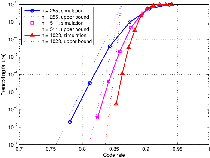
Fig. 4 shows that the upper bound is very close to the simulation results when the probability of encoding failure is low. In regards to the simulation results, we used PBCH codes for the BDC with $\beta=0.1$.

For the BDEC, the encoder should try to mask stuck-at defects and the decoder should correct erasures. The encoding process of the BDEC is the same as the encoding in 2.2. Only the decoding will be modified as follows.

Decoding (BDEC): The MLD is done by solving the following linear equation.

where ${\mathcal{V}}=\left\{j_{1},\cdots,j_{v}\right\}$ indicates the locations of $v$ unerased bits. We use the notation of ${\mathbf{y}}^{\mathcal{V}}=\left(y_{j_{1}},\cdots,y_{j_{v}}\right)^{T}$ and $\widetilde{G}^{\mathcal{V}}=\left[\widetilde{\mathbf{g}}_{j_{1}}^{T},\cdots,\widetilde{\mathbf{g}}_{j_{v}}^{T}\right]^{T}$ where $\widetilde{\mathbf{g}}_{j}$ is the $j$-th row of $\widetilde{G}$. By solving (36), we can obtain estimates of the message $\mathbf{m}$ and redundancy $\mathbf{d}$, i.e., $\widehat{\mathbf{m}}$ and $\widehat{\mathbf{d}}$. We consider the MLD in order to derive the upper bound on $P\left(\widehat{\mathbf{m}}\neq\mathbf{m}\right)$. The MLD can be accomplished by solving the linear equation in (36), whose complexity is ${\mathcal{O}}\left(n^{3}\right)$.

where $\alpha$ is the probability of erasure and $\beta$ is the probability of defect for the BDEC.

Fig. 2 represents the capacity region by Theorem 3.19. The supremum of $R_{1}$ in this capacity region is $1-\alpha-\beta$ which is equal to $C_{\text{BDEC}}^{\text{enc}}$ of (13). From (37), we can obtain $l>n\beta$ and $r>n\alpha$, which achieve the capacity for infinite $n$.

As explained earlier, these asymptotic results cannot be directly used to choose the optimal redundancy allocation $\left(l^{*},r^{*}\right)$ of (2) for finite-length codes. We emphasize that the optimal redundancy allocation $\left(l^{*},r^{*}\right)$ is equivalent to finding the optimal (i.e., minimizing the probability of recovery error) point in the capacity region in Fig. 2.

In order to solve the optimization problem of (2), we need a closed-form expression for $P\left(\widehat{\mathbf{m}}\neq\mathbf{m}\right)$. Unfortunately, it is difficult to obtain the exact expression of $P\left(\widehat{\mathbf{m}}\neq\mathbf{m}\right)$. Thus, we will consider an estimate $(\widehat{l},\widehat{r})$ which minimizes an upper bound on $P\left(\widehat{\mathbf{m}}\neq\mathbf{m}\right)$.

In this upper bound, we observe a dual relation between erasures and defects [21]. Note that $A_{w}$ and $B_{0,w}$ are the weight distributions of $\mathcal{C}$ and ${\mathcal{C}}_{0}^{\perp}$, respectively.

From these upper bounds on $P\left(\widehat{\mathbf{m}}\neq\mathbf{m}\right)$, we can modify (2) for the BDEC as follows.

If the code parameters $(n,k,l,d_{0},d_{1})$ and the channel parameters ($\alpha$, $\beta$) are given, the solution $(\widehat{l},\widehat{r})$ of (41) can be obtained. To illustrate this, we consider $\left[n=1023,k=923,l\right]$ PBCH codes. All possible redundancy allocation candidates of PBCH codes are listed in Table 1. Since $l$ and $r$ are multiples of 10 (i.e., the degree of the Galois field of $[n=1023,k]$ BCH codes), there are 11 redundancy allocation candidates. Hence, we can readily obtain the redundancy $(\widehat{l},\widehat{r})$ that minimizes the objective function of (41).

In addition, the objective function is convex if we treat $l$ and $r$ as real values, even though we know that they are non-negative integers less than or equal to $n-k$. We can derive the solution $(\widetilde{l},\widetilde{r})$ of (41) satisfying Karush-Kuhn-Tucker (KKT) conditions.

If $\alpha$ is much larger than $\beta$ such that $\frac{1+\alpha}{1+\beta}>2^{1-R}$ for all possible $(l,r)$, then (42) shows that we should allot all redundancy for correcting erasures to minimize the upper bound of (41). If $\beta$ is much larger than $\alpha$ such that $\frac{1+\alpha}{1+\beta}<2^{-(1-R)}$ for all possible $(l,r)$, then (44) shows that we should allot all redundancy for masking stuck-at defects to minimize the upper bound. For other $\alpha$ and $\beta$, we should allot the redundancy $(l,r)$ such that $2^{-l}\left(1+\beta\right)^{n}=2^{-r}\left(1+\alpha\right)^{n}$ to minimize the upper bound, which are satisfied by (45) and (46).

In order to compare the optimal redundancy and the estimated redundancy allocation based on the derived upper bound, we consider several channels in Table 2 whose capacities are all equal, i.e., $C_{\text{BDEC}}^{\text{enc}}=0.96$. For these channels, we investigate the performance of $\left[n=1023,k=923,l\right]$ PBCH codes in Table 1.

Fig. 5 shows the simulation results for the channels in Table 2. The simulation results of channel 1 (BEC) and channel 7 (BDC) are omitted because their optimal redundancy allocations are obvious. The optimal redundancy allocation for channel 1 (BEC) is $\left(l^{*},r^{*}\right)=(0,100)$. The more stuck-at defects a channel has, the larger $l$ is expected to be for the optimal redundancy allocation. Eventually, the optimal redundancy allocation for channel 7 (BDC) will be $\left(l^{*},r^{*}\right)=(100,0)$. The optimal $\left(l^{*},r^{*}\right)$ can be obtained from Monte-Carlo simulation results in Fig. 5, which are presented in the second column of Table 5.

We can readily obtain the redundancy $(\widehat{l},\widehat{r})$ that minimizes the upper bounds in Fig. 5. The estimates of redundancy allocation $(\widehat{l},\widehat{r})$ are shown in the third column of Table 3 which shows that $(\widehat{l},\widehat{r})$ by the upper bounds matches very well the redundancy $(l^{*},r^{*})$ determined by Monte-Carlo simulations.

Next, $(\widetilde{l},\widetilde{r})$ can be calculated from (42)–(46) by treating $l$ and $r$ as real values. Resulting $(\widetilde{l},\widetilde{r})$ values are shown in the last column of Table 3. $(\widehat{l},\widehat{r})$ is the nearest one from $(\widetilde{l},\widetilde{r})$ considering the possible redundancy allocation candidates in Table 1.

A similar approach to redundancy allocation of the BDEC will be used for the BDSC. Instead of minimizing the upper bound on $P\left(\widehat{\mathbf{m}}\neq\mathbf{m}\right)$, we will derive an estimate of $P\left(\widehat{\mathbf{m}}\neq\mathbf{m}\right)$ for the BDSC and the redundancy allocation $(l,r)$ that minimizes this estimate of $P\left(\widehat{\mathbf{m}}\neq\mathbf{m}\right)$ will be used.

For the BDC and the BDEC, the number of unmasked defects after encoding failure (i.e., $\mathbf{c}\circ\mathbf{s}\neq\mathbf{c}$) does not affect $P\left(\widehat{\mathbf{m}}\neq\mathbf{m}\right)$. On the other hand, the number of unmasked defects is important for $P\left(\widehat{\mathbf{m}}\neq\mathbf{m}\right)$ of the BDSC. The reason is that the stuck-at errors due to unmasked defects can be treated as random errors and corrected during the decoding stage. Hence, we propose a two-step encoding method (described in Algorithm 1), which reduces the performance gap between (19) and (20).

The two-step encoding tries to reduce the number of unmasked defects by using the second step (i.e., Step 2) even though $\mathbf{c}\circ\mathbf{s}\neq\mathbf{c}$. When the encoder fails to solve (20), the encoder randomly chooses $d_{0}-1$ defect locations among $\mathcal{U}$ and define ${\mathcal{U}}^{\prime}=\left\{i_{1},\ldots,i_{d_{0}-1}\right\}$. Afterwards, the encoder solves $G_{0}^{\mathcal{U}^{\prime}}{\mathbf{d}}={\mathbf{b}}^{\mathcal{U}^{\prime}}$ where a solution $\mathbf{d}$ always exists by the definition of $d_{0}$ in (18). If $\mathbf{d}$ is obtained in Step 2, then the number of unmasked defects is $u-\left(d_{0}-1\right)$ instead of $u$. For the BDC and the BDEC, Step 2 cannot improve $P(\widehat{\mathbf{m}}\neq\mathbf{m})$ since unmasked stuck-at defects cannot be corrected during the decoding stage. However, Step 2 is helpful for the BDSC since the stuck-at errors can be regarded as random errors and corrected at the decoder.

The two-step encoding’s complexity is ${\mathcal{O}}\left(u^{3}\right)$ because both Step 1 and Step 2 are related to solving the linear equations. Also, the bounded distance decoding for estimating $\widehat{\mathbf{z}}$ can be implemented by polynomial decoding algorithms. For PBCH codes, standard algorithms such as Berlekamp-Massey algorithm can be used for decoding. The flow of PLBC’s decoding for the BDSC was explained in Section 2.2.

We will derive the upper bound on $P\left(\widehat{\mathbf{m}}\neq\mathbf{m}\right)$ where the two-step encoding and the bounded distance decoding are used.

During the derivation of the upper bound of (47), we regard all the unmasked stuck-at defects as random errors. However, on average, only half of the unmasked defects result in error if $P(S=0)=P(S=1)=\frac{\beta}{2}$. Thus, we can derive the following estimate of $P\left(\widehat{\mathbf{m}}\neq\mathbf{m}\right)$.

References

- [1] A. V. Kuznetsov and B. S. Tsybakov, “Coding in a memory with defective cells,” Probl. Peredachi Inf., vol. 10, no. 2, pp. 52–60, Apr.–Jun. 1974.
- [2] A. El Gamal and Y.-H. Kim, Network Information Theory. Cambridge, U.K.: Cambridge University Press, 2011.
- [3] C. Heegard and A. El Gamal, “On the capacity of computer memory with defects,” IEEE Trans. Inf. Theory, vol. 29, no. 5, pp. 731–739, Sep. 1983.
- [4] B. S. Tsybakov, “Additive group codes for defect correction,” Probl. Peredachi Inf., vol. 11, no. 1, pp. 111–113, Jan.–Mar. 1975.
- [5] I. I. Dumer, “Asymptotically optimal linear codes correcting defects of linearly increasing multiplicity.” Probl. Peredachi Inf., vol. 26, no. 2, pp. 93–104, Apr.–Jun. 1990.
- [6] L. A. Lastras-Montano, A. Jagmohan, and M. M. Franceschini, “Algorithms for memories with stuck cells,” in Proc. IEEE Int. Symp. Inf. Theory (ISIT), Jun. 2010, pp. 968–972.
- [7] A. Jagmohan, L. A. Lastras-Montano, M. M. Franceschini, M. Sharma, and R. Cheek, “Coding for multilevel heterogeneous memories,” in Proc. IEEE Int. Conf. Commun. (ICC), May 2010, pp. 1–6.
- [8] E. Hwang, B. Narayanaswamy, R. Negi, and B. V. K. Vijaya Kumar, “Iterative cross-entropy encoding for memory systems with stuck-at errors,” in Proc. IEEE Global Commun. Conf. (GLOBECOM), Dec. 2011, pp. 1–5.
- [9] A. N. Jacobvitz, R. Calderbank, and D. J. Sorin, “Coset coding to extend the lifetime of memory,” in Proc. 19th IEEE Int. Symp. on High Performance Comput. Archi. (HPCA), Feb. 2013, pp. 222–233.
- [10] Y. Kim and B. V. K. Vijaya Kumar, “Coding for memory with stuck-at defects,” in Proc. IEEE Int. Conf. Commun. (ICC), Jun. 2013, pp. 4347–4352.
- [11] Y. Kim and B. V. K. Vijaya Kumar, “Redundancy allocation of partitioned linear block codes,” in Proc. IEEE Int. Symp. Inf. Theory (ISIT), Jul. 2013, pp. 2374–2378.
- [12] H. Mahdavifar and A. Vardy, “Explicit capacity achieving codes for defective memories,” in Proc. IEEE Int. Symp. Inf. Theory (ISIT), Jun. 2015, pp. 641–645.
- [13] Y. Kim, A. A. Sharma, R. Mateescu, S.-H. Song, Z. Z. Bandic, J. A. Bain, and B. V. K. Vijaya Kumar, “Locally rewritable codes for resistive memories,” IEEE J. Sel. Areas Commun. (JSAC), vol. 34, no. 9, pp. 2470–2485, Sep. 2016.
- [14] A. Pirovano, A. Redaelli, F. Pellizzer, F. Ottogalli, M. Tosi, D. Ielmini, A. L. Lacaita, and R. Bez, “Reliability study of phase-change nonvolatile memories,” IEEE Trans. Device Mater. Rel., vol. 4, no. 3, pp. 422–427, Sep. 2004.
- [15] Y. Kim and B. V. K. Vijaya Kumar, “Writing on dirty flash memory,” in Proc. 52nd Annu. Allerton Conf. Commun., Control, Comput., Oct. 2014, pp. 513–520.
- [16] B. S. Tsybakov, “Defect and error correction,” Probl. Peredachi Inf., vol. 11, no. 3, pp. 21–30, Jul.–Sep. 1975.
- [17] K. Prall, “Scaling non-volatile memory below 30nm,” in Proc. IEEE Non-Volatile Semiconductor Memory Workshop, Aug. 2007, pp. 5–10.
- [18] C. Heegard, “Partitioned linear block codes for computer memory with “stuck-at” defects,” IEEE Trans. Inf. Theory, vol. 29, no. 6, pp. 831–842, Nov. 1983.
- [19] R. Zamir, S. Shamai, and U. Erez, “Nested linear/lattice codes for structured multiterminal binning,” IEEE Trans. Inf. Theory, vol. 48, no. 6, pp. 1250–1276, Jun. 2002.
- [20] F. J. MacWilliams and N. J. A. Sloane, The Theory of Error-Correcting Codes. Amsterdam, The Netherlands: North-Holland, 1977, pp. 282–283.
- [21] Y. Kim and B. V. K. Vijaya Kumar, “Duality between erasures and defects,” in Proc. Inf. Theory Appl. Workshop (ITA), Feb. 2016, pp. 1–10.
- [22] S. I. Gelfand and M. S. Pinsker, “Coding for channel with random parameters,” Probl. Contr. and Inf. Theory, vol. 9, no. 1, pp. 19–31, 1980.