跳到论文正文
W Papers独立论文阅读器 arXiv:1802.10365 论文正文 计算阅读时间 · 0%
引用这篇论文根据当前论文元数据生成,正式投稿前建议核对。


License: arXiv.org perpetual non-exclusive license
arXiv:1802.10365v2 [cond-mat.str-el] 16 May 2019

Topological quantum critical point in triple-Weyl semimetal: non-Fermi-liquid behaviors and instabilities

Jing-Rong Wang Affiliation: Anhui Province Key Laboratory of Condensed Matter Physics at Extreme Conditions, High Magnetic Field Laboratory of the Chinese Academy of Sciences, Hefei, Anhui 230031, China    Guo-Zhu Liu Affiliation: Corresponding author: gzliu@ustc.edu.cn Affiliation: Department of Modern Physics, University of Science and Technology of China, Hefei, Anhui 230026, China    Chang-Jin Zhang Affiliation: Corresponding author: zhangcj@hmfl.ac.cn Affiliation: Anhui Province Key Laboratory of Condensed Matter Physics at Extreme Conditions, High Magnetic Field Laboratory of the Chinese Academy of Sciences, Hefei, Anhui 230031, China Affiliation: Institute of Physical Science and Information Technology, Anhui University, Hefei, Anhui 230601, China
Abstract

We study the quantum critical phenomena emerging at the transition from triple-Weyl semimetal to band insulator, which is a topological phase transition described by the change of topological invariant. The critical point realizes a new type of semimetal state in which the fermion dispersion is cubic along two directions and quadratic along the third. Our renormalization group analysis reveals that, the Coulomb interaction is marginal at low energies and even arbitrarily weak Coulomb interaction suffices to induce an infrared fixed point. We compute a number of observable quantities, and show that they all exhibit non-Fermi liquid behaviors at the fixed point. When the interplay between the Coulomb and short-range four-fermion interactions is considered, the system becomes unstable below a finite energy scale. The system undergoes a first-order topological transition when the fermion flavor NN is small, and enters into a nematic phase if NN is large enough. Non-Fermi liquid behaviors are hidden by the instability at low temperatures, but can still be observed at higher temperatures. Experimental detection of the predicted phenomena is discussed.

I Introduction

Weakly interacting fermion systems are well described by Fermi liquid (FL) theory [1, 2]. Inter-particle interactions induce a variety of continuous phase transitions, such as magnetically ordered transition [3, 4], charge-density-wave transition [5], and nematic transition [6]. This type of transition happens between two phases with distinct symmetries. According to Ginzburg-Landau-Wilson (GLW) theory [3], one can define a local order parameter to describe such a transition. At the quantum critical point (QCP), fermionic excitations interact strongly with the quantum fluctuation of order parameter, which often leads to breakdown of FL theory [3, 4, 5, 6, 7]. However, not all phase transitions are classified by the change of symmetries. Transitions may occur between phases that respect the same symmetries but are topologically distinct [8, 9]. These transitions are beyond the paradigm of GLW theory, and could be described by the change of global topological invariant.

In recent years, a plethora of semimetal (SM) materials have been discovered and extensively investigated [10, 11, 12, 13, 14, 15, 16, 17, 18, 19, 20]. Under suitable conditions, SM states emerge at the toplogical QCP (TQCP) between two topologically distinct phases [21, 23, 22, 24, 28, 25, 26, 27, 29, 30, 31, 32, 33]. For instance, three-dimensional (3D) topological insulator (TI) can be turned into a band insulator (BI), with gapless 3D Dirac SM (DSM) state emerging at TI-BI QCP [21, 23, 34, 35].

Inter-particle interaction effect at TQCP is a nontrivial issue and has attracted particular interest recently [23, 24, 25, 26, 31]. The fermions do not couple to any order parameter at the TQCP. Their properties are determined mainly by the Coulomb interaction, which is long-ranged because the density of states (DOS) vanishes at Fermi level. The effects of Coulomb interaction are diverse in various SM systems, depending sensitively on the spatial dimensionality and the fermion energy dispersion [23, 24, 25, 26, 31, 36, 37, 38, 39, 40, 41, 42, 43, 44].

In this article, we consider the transition between topological triple-Weyl SM (WSM) and BI. In a triple-WSM, the fermion energy spectrum disperses cubically along two directions and linearly along the third one, and the monopole charges of one pair of Weyl points are ±3\pm 3 [42, 43, 44, 45, 46, 47, 48, 49, 50, 51, 52, 53, 54]. In the process of turning triple-WSM into BI, two Weyl points carrying opposite monopole charges merge to form one single band-touching point that carries zero monopole charge. This is a topological quantum phase transition (TQPT) since the monopole charge is finite in one phase and zero in the other. The merging process is shown in Fig. 1. At the TQCP, the fermion dispersion is cubic along two directions and quadratic along the third, which defines a new gapless SM state.

We investigate the influence of long-range Coulomb interaction on the triple-WSM-BI TQCP by carrying out an extensive renormalization group (RG) analysis. The Coulomb interaction is found to be marginal in the low-energy regime. The system flows to an infrared fixed point, at which the interaction strength takes a finite value. We compute a number of observable quantities and demonstrate that they all exhibit striking non-FL (NFL) behaviors at such a fixed point.

Refer to caption
Figure 1: As a triple-WSM is converted into a normal BI, two band-touching points merge to one single point at the TQCP. The fermion dispersion can be universally expressed in the form E=±B2​k⊥6+(A​kz2−Δ)2E=\pm\sqrt{B^{2}k_{\bot}^{6}+\left(Ak_{z}^{2}-\Delta\right)^{2}}. (a) BI with Δ<0\Delta<0; (b) TQCP with Δ=0\Delta=0; (c) Triple-WSM with Δ>0\Delta>0.

We then study the possible instabilities of this fixed point by analyzing the interplay between the Coulomb interaction and some sorts of short-range four-fermion interactions. Our finding is that, the system undergoes a first order TQPT when the fermion flavor NN is small and develops a nematic order if NN is sufficiently large. The NFL behaviors are hidden at low temperatures due to the instability, but still have observable effects at higher temperatures. All these results, summarized in the schematic phase diagram given by Fig. 2, can be verified by experiments.

The rest of the paper will be organized as follows. In Sec. II, the effective low-energy action of the TQCP is introduced and described. In Sec. III, the coupled RG equations for model parameters are presented, and the RG solutions are analyzed. The NFL behaviors of observable quantities are discussed in Sec. IV. The possible phase-transition instabilities induced by the Coulomb and short-range interactions are investigated in Sec. V. In Sec. VI, the experimental detection of our theoretical predictions is briefly discussed. All of calculational details are presented in the Appendices.

II The model

At the triple-WSM-BI TQCP, the free Hamiltonian of the gapless fermions takes the form

Hf=∑i=13∫d3​𝐱​ψa†​(𝐱)​di​(𝐱)​σi​ψa​(𝐱),H_{f}=\sum_{i=1}^{3}\int d^{3}\mathbf{x}\psi_{a}^{{\dagger}}(\mathbf{x})d_{i}(\mathbf{x})\sigma_{i}\psi_{a}(\mathbf{x}), (1)

where d1(𝐱)=Bi(∂x3−3∂x∂y2)d_{1}(\mathbf{x})=Bi(\partial_{x}^{3}-3\partial_{x}\partial_{y}^{2}), d2(𝐱)=Bi(∂y3−3∂y∂x2)d_{2}(\mathbf{x})=Bi(\partial_{y}^{3}-3\partial_{y}\partial_{x}^{2}), and d3(𝐱)=−A∂z2d_{3}(\mathbf{x})=-A\partial_{z}^{2}. The field operator ψa\psi_{a} is a two-component spinor, and repeated indices of aa implies the summation from 11 to NN, where NN is the fermion flavor. σ1,2,3\sigma_{1,2,3} are the Pauli matrices, and BB and AA are model parameters. The fermion energy dispersion is E=±B2​k⊥6+A2​kz4E=\pm\sqrt{B^{2}k_{\bot}^{6}+A^{2}k_{z}^{4}}, where k⊥2=kx2+ky2k_{\bot}^{2}=k_{x}^{2}+k_{y}^{2}. The Coulomb interaction can be described by

HC=14​π​∫d3​𝐱​d3​𝐱′​ρa​(𝐱)​e2ϵ​|𝐱−𝐱′|​ρa​(𝐱′),\displaystyle H_{C}=\frac{1}{4\pi}\int d^{3}\mathbf{x}d^{3}\mathbf{x}^{\prime}\rho_{a}(\mathbf{x})\frac{e^{2}}{\epsilon\left|\mathbf{x}-\mathbf{x}^{\prime}\right|}\rho_{a}(\mathbf{x}^{\prime}), (2)

where ρa​(𝐱)=ψa†​(𝐱)​ψa​(𝐱)\rho_{a}(\mathbf{x})=\psi_{a}^{{\dagger}}(\mathbf{x})\psi_{a}(\mathbf{x}) is fermion density operator, ee electric charge, and ϵ\epsilon dielectric constant. One can treat Coulomb interaction by defining an auxiliary boson field ϕ\phi via the Hubbard-Stratonovich transformation [23, 24, 25, 31, 42, 43, 36, 37, 38, 39, 40, 41].

Refer to caption
Figure 2: Phase diagram on mm-TT plane, where mm tunes the transition and TT is temperature. The TQCP (mcm_{c}) is broadened into a NFL-like quantum critical regime at finite TT. Magenta dome appearing at low TT represents either the formation of nematic order or the occurrence of first-order TQPT.

The total effective action is formally expressed as S=Sψ+Sϕ+Sψ​ϕS=S_{\psi}+S_{\phi}+S_{\psi\phi}, where

Sψ\displaystyle S_{\psi} =\displaystyle= ∫d​ω2​π​d3​𝐤(2​π)3​ψa†​(i​ω−ℋf​(𝐤))​ψa,\displaystyle\int\frac{d\omega}{2\pi}\frac{d^{3}\mathbf{k}}{(2\pi)^{3}}\psi_{a}^{{\dagger}}\left(i\omega-\mathcal{H}_{f}(\mathbf{k})\right)\psi_{a}, (3)
Sϕ\displaystyle S_{\phi} =\displaystyle= ∫d​ω2​π​d3​𝐤(2​π)3​ϕ​(k⊥2+η​kz2)​ϕ,\displaystyle\int\frac{d\omega}{2\pi}\frac{d^{3}\mathbf{k}}{(2\pi)^{3}}\phi\left(k_{\bot}^{2}+\eta k_{z}^{2}\right)\phi, (4)
Sψ​ϕ\displaystyle S_{\psi\phi} =\displaystyle= i​g​∫d​τ​d3​𝐱​ϕ​ψa†​ψa.\displaystyle ig\int d\tau d^{3}\mathbf{x}\phi\psi_{a}^{{\dagger}}\psi_{a}. (5)

Here, g=4​π​e/ϵg=\sqrt{4\pi}e/\sqrt{\epsilon}. Because the fermion dispersion is anisotropic, the three momentum components need to be re-scaled differently. To facilitate RG calculations, we have introduced a parameter η\eta. The bare fermion propagator is given by

G0​(i​ω,𝐤)=1i​ω−d1​(𝐤)​σ1−d2​(𝐤)​σ2−d3​(𝐤)​σ3,\displaystyle G_{0}(i\omega,\mathbf{k})=\frac{1}{i\omega-d_{1}(\mathbf{k})\sigma_{1}-d_{2}(\mathbf{k})\sigma_{2}-d_{3}(\mathbf{k})\sigma_{3}}, (6)

where d1​(𝐤)=B⁡(kx3−3​kx​ky2)d_{1}(\mathbf{k})=B\left(k_{x}^{3}-3k_{x}k_{y}^{2}\right), d2​(𝐤)=B⁡(ky3−3​ky​kx2)d_{2}(\mathbf{k})=B\left(k_{y}^{3}-3k_{y}k_{x}^{2}\right), and d3​(𝐤)=A​kz2d_{3}(\mathbf{k})=Ak_{z}^{2}. The bare boson propagator reads

D0​(𝐪)=1q⊥2+η​qz2,\displaystyle D_{0}(\mathbf{q})=\frac{1}{q_{\bot}^{2}+\eta q_{z}^{2}}, (7)

which is clearly long-ranged.

III Renormalization group analysis

We now employ the RG method [55] to study the Coulomb interaction on the low-energy properties of fermions. The momentum shell to be integrated out is chosen as b​Λ<B2​k⊥6+A2​kz4<Λb\Lambda<\sqrt{B^{2}k_{\bot}^{6}+A^{2}k_{z}^{4}}<\Lambda, where Λ\Lambda is some high-energy cutoff and b=e−ℓb=e^{-\ell} with ℓ\ell being the flow parameter. After performing tedious calculations, we obtain the fermion self-energy

Σ⁡(i​ω,𝐤)≈−[d1​(𝐤)​σ1+d2​(𝐤)​σ2]​C2​ℓ−A​kz2​σ3​C3​ℓ.\displaystyle\Sigma(i\omega,\mathbf{k})\approx-\left[d_{1}(\mathbf{k})\sigma_{1}+d_{2}(\mathbf{k})\sigma_{2}\right]C_{2}\ell-Ak_{z}^{2}\sigma_{3}C_{3}\ell. (8)

The expressions of C2C_{2} and C3C_{3} are complicated and can be found in Appendix A. According to Appendix B, the boson self-energy calculated in the static limit is given by

Π⁡(𝐪)≈q⊥2​C⊥​ℓ+qz2​Cz​ℓ,\displaystyle\Pi(\mathbf{q})\approx q_{\bot}^{2}C_{\bot}\ell+q_{z}^{2}C_{z}\ell, (9)

where

C⊥\displaystyle C_{\bot} =\displaystyle= 9​g240​π2​A​Λ,\displaystyle\frac{9g^{2}}{40\pi^{2}\sqrt{A\Lambda}}, (10)
Cz\displaystyle C_{z} =\displaystyle= Γ⁡(34)​Γ​(43)​g2​A24​π2​Γ​(2512)​B2/3​Λ5/6.\displaystyle\frac{\Gamma\left(\frac{3}{4}\right)\Gamma\left(\frac{4}{3}\right)g^{2}\sqrt{A}}{24\pi^{2}\Gamma\left(\frac{25}{12}\right)B^{2/3}\Lambda^{5/6}}. (11)

According to the calculations presented in Appendix C, the coupled RG equations for model parameters are

d​Bd​ℓ\displaystyle\frac{dB}{d\ell} =\displaystyle= C2​B,\displaystyle C_{2}B, (12)
d​Ad​ℓ\displaystyle\frac{dA}{d\ell} =\displaystyle= C3​A,\displaystyle C_{3}A, (13)
d​αd​ℓ\displaystyle\frac{d\alpha}{d\ell} =\displaystyle= (12−N​C⊥−C32)​α,\displaystyle\left(\frac{1}{2}-NC_{\bot}-\frac{C_{3}}{2}\right)\alpha, (14)
d​βd​ℓ\displaystyle\frac{d\beta}{d\ell} =\displaystyle= (56+12​C3−23​C2−N​β)​β,\displaystyle\left(\frac{5}{6}+\frac{1}{2}C_{3}-\frac{2}{3}C_{2}-N\beta\right)\beta, (15)
d​ηd​ℓ\displaystyle\frac{d\eta}{d\ell} =\displaystyle= (−13−N​C⊥+N​β)​η,\displaystyle\left(-\frac{1}{3}-NC_{\bot}+N\beta\right)\eta, (16)
d​ζd​ℓ\displaystyle\frac{d\zeta}{d\ell} =\displaystyle= (−13+23​C2−C3−N​C⊥+N​β)​ζ.\displaystyle\left(-\frac{1}{3}+\frac{2}{3}C_{2}-C_{3}-NC_{\bot}+N\beta\right)\zeta. (17)

Here, we define three new parameters: α=5​C⊥/9​π\alpha=5C_{\bot}/9\pi, β=Cz/η\beta=C_{z}/\eta, and ζ=η​B2/3​Λ1/3/A\zeta=\eta B^{2/3}\Lambda^{1/3}/A. The parameter α\alpha represents the effective Coulomb interaction strength, whereas the parameter β\beta is related to the dynamical screening of Coulomb interaction. In our RG calculations, 1/N1/N serves as a formal control parameter.

Refer to caption
Figure 3: Flow diagram on α\alpha-β\beta plane for N=1N=1 is given in (a) and for N=2N=2 in (b). Red point (α∗,β∗)(\alpha^{*},\beta^{*}) is an infrared fixed point. (c) and (d) show the NN-dependence of some parameters.

We plot the flow diagrams on the α\alpha-β\beta plane in Figs. 3(a) and 3(b) based on the solutions of Eqs. (12)-(17). There is a stable infrared fixed point (α∗,β∗)(\alpha^{*},\beta^{*}). In the lowest energy limit, C2C_{2}, C3C_{3}, and C⊥C_{\bot} approach to three constants C2∗C_{2}^{*}, C3∗C_{3}^{*}, and C⊥∗C_{\bot}^{*}, respectively. The values of the constants α∗\alpha^{*}, β∗\beta^{*}, C2∗C_{2}^{*}, C3∗C_{3}^{*}, and C⊥∗C_{\bot}^{*} are shown in Fig. 3(c), and can be found in Appendix C. The constant C3∗<0C_{3}^{*}<0, but other constants are positive. At low energies, the parameters BB and AA behave as

B\displaystyle B ∼\displaystyle\sim eC2∗​ℓ,\displaystyle e^{C_{2}^{*}\ell}, (18)
A\displaystyle A ∼\displaystyle\sim eC3∗​ℓ.\displaystyle e^{C_{3}^{*}\ell}. (19)

As the energy decreases, BB increases indefinitely, while AA goes to zero quickly. Since BB and AA enter into almost all the observable quantities, such a renormalization will certainly have observable effects.

Including polarization Π⁡(𝐪)\Pi(\mathbf{q}) into the boson propagator leads to renormalized Coulomb interaction

D⁡(𝐪)=1D0−1​(𝐪)+Π⁡(𝐪)∼1q⊥2−3​N​C⊥∗+qz2−2​N​β∗.\displaystyle D(\mathbf{q})=\frac{1}{D_{0}^{-1}(\mathbf{q})+\Pi(\mathbf{q})}\sim\frac{1}{q_{\bot}^{2-3NC_{\bot}^{*}}+q_{z}^{2-2N\beta^{*}}}. (20)

Since C⊥∗C_{\bot}^{*} and β∗\beta^{*} are both positive, the Coulomb interaction is substantially screened.

IV Observable Quantities

The infrared fixed point (α∗,β∗)(\alpha^{*},\beta^{*}) is characterized by the emergence of striking NFL behaviors. To demonstrate this, we will compute a number of observable quantities, including the fermion DOS, specific heat, compressibility, dynamical conductivities, and diamagnetic susceptibilities. The detailed calculations of observable quantities can be found in Appendices D and E.

Table 1: The energy or temperature dependence of observable quantities at TQCP between triple-WSM and BI. The interaction-induced extra exponents are shown in Fig. 3(d) and also in Appendix E

.

ρ⁡(ω)\rho(\omega) Cv​(T)C_{v}(T) κ⁡(T)\kappa(T) σ⊥⁣⊥​(ω)\sigma_{\bot\bot}(\omega) σz​z​(ω)\sigma_{zz}(\omega) χD⊥​(T)\chi_{D}^{\bot}(T) χDz​(T)\chi_{D}^{z}(T)
Free ω1/6\omega^{1/6} T7/6T^{7/6} T1/6T^{1/6} ω1/2\omega^{1/2} ω1/6\omega^{1/6} T1/2T^{1/2} T5/6T^{5/6}
Interacting ω1/6+η1\omega^{1/6+\eta_{1}} T7/6+η1T^{7/6+\eta_{1}} T1/6+η1T^{1/6+\eta_{1}} ω1/2+η2\omega^{1/2+\eta_{2}} ω1/6+η3\omega^{1/6+\eta_{3}} T1/2+η4T^{1/2+\eta_{4}} T5/6+η5T^{5/6+\eta_{5}}

We first consider the non-interacting limit. It is easy to get the fermion DOS

ρ⁡(ω)=c1A​B2/3​ω1/6.\displaystyle\rho(\omega)=\frac{c_{1}}{\sqrt{A}B^{2/3}}\omega^{1/6}. (21)

Apparently, ρ⁡(ω)\rho(\omega) vanishes in the limit ω→0\omega\rightarrow 0, which is a common feature of most SMs and renders that the Coulomb interaction is long-ranged. The specific heat Cv​(T)C_{v}(T) and compressibility κ⁡(T)\kappa(T) are

Cv​(T)\displaystyle C_{v}(T) =\displaystyle= c2A​B2/3​T7/6,\displaystyle\frac{c_{2}}{\sqrt{A}B^{2/3}}T^{7/6}, (22)
κ⁡(T)\displaystyle\kappa(T) =\displaystyle= c3A​B2/3​T1/6,\displaystyle\frac{c_{3}}{\sqrt{A}B^{2/3}}T^{1/6}, (23)

respectively. The dynamical conductivity within xx-yy plane, σ⊥⁣⊥​(ω)\sigma_{\bot\bot}(\omega), and the one along zz-axis, σz​z​(ω)\sigma_{zz}(\omega), are

σ⊥⁣⊥​(ω)\displaystyle\sigma_{\bot\bot}(\omega) =\displaystyle= c4​e2A​ω1/2,\displaystyle\frac{c_{4}e^{2}}{\sqrt{A}}\omega^{1/2}, (24)
σz​z​(ω)\displaystyle\sigma_{zz}(\omega) =\displaystyle= c5​A​e2B2/3​ω1/6.\displaystyle\frac{c_{5}\sqrt{A}e^{2}}{B^{2/3}}\omega^{1/6}. (25)

For the external fields applied within the xx-yy plane and along the zz-axis, the diamagnetic susceptibilities are respectively given by

Δ​χD⊥​(T)\displaystyle\Delta\chi_{D}^{\bot}(T) =\displaystyle= c6​A​e2​T1/2,\displaystyle c_{6}\sqrt{A}e^{2}T^{1/2}, (26)
Δ​χDz​(T)\displaystyle\Delta\chi_{D}^{z}(T) =\displaystyle= c7​B2/3​e2A​T5/6,\displaystyle c_{7}\frac{B^{2/3}e^{2}}{\sqrt{A}}T^{5/6}, (27)

where Δ​χD⊥​(T)=χD⊥​(T)−χD​0⊥\Delta\chi_{D}^{\bot}(T)=\chi_{D}^{\bot}(T)-\chi_{D0}^{\bot} and Δ​χDz​(T)=χDz​(T)−χD​0z\Delta\chi_{D}^{z}(T)=\chi_{D}^{z}(T)-\chi_{D0}^{z}, with χD​0⊥\chi_{D0}^{\bot} and χD​0z\chi_{D0}^{z} being the residual values of the T→0T\rightarrow 0 limit. The values of constants c1c_{1}, c2c_{2}, …, c7c_{7} are given in Appendix D.

We then incorporate the corrections induced by the Coulomb interaction. Making use of the RG results of B⁡(ℓ)B(\ell) and A⁡(ℓ)A(\ell), and then employing the scaling relation ω=ω0​e−ℓ\omega=\omega_{0}e^{-\ell} or T=T0​e−ℓT=T_{0}e^{-\ell}, we can obtain the renormalized observable quantities. First of all, the DOS becomes

ρ⁡(ω)∼ω1/6+η1,\displaystyle\rho(\omega)\sim\omega^{1/6+\eta_{1}}, (28)

where η1>0\eta_{1}>0. Comparing Eq. (21) to Eq. (28), we find that Coulomb interaction effectively suppresses fermion DOS. Interaction corrections modify specific heat and compressibility to

Cv​(T)\displaystyle C_{v}(T) ∼\displaystyle\sim T7/6+η1,\displaystyle T^{7/6+\eta_{1}}, (29)
κ⁡(T)\displaystyle\kappa(T) ∼\displaystyle\sim T1/6+η1.\displaystyle T^{1/6+\eta_{1}}. (30)

These two quantities are also suppressed. The extra exponent η1\eta_{1} appearing in ρ⁡(ω)\rho(\omega), Cv​(T)C_{v}(T), and κ⁡(T)\kappa(T) is exactly the same, which reflects the fact that ρ⁡(ω)\rho(\omega), Cv​(T)C_{v}(T), and κ⁡(T)\kappa(T) display the same dependence on BB and AA, as shown in Eqs. (21), (22), and (23).

According to Eqs. (24)- (27), the charge ee enters into the expressions of dynamical conductivities and diamagnetic susceptibilities. The RG flow of ee naturally affects the low-energy properties of these quantities. From the ℓ\ell-dependence of BB, AA, and ee, we find that

σ⊥⁣⊥​(ω)\displaystyle\sigma_{\bot\bot}(\omega) ∼\displaystyle\sim ω1/2+η2,\displaystyle\omega^{1/2+\eta_{2}}, (31)
σz​z​(ω)\displaystyle\sigma_{zz}(\omega) ∼\displaystyle\sim ω1/6+η3,\displaystyle\omega^{1/6+\eta_{3}}, (32)

where η2=0\eta_{2}=0 and η3\eta_{3} is a positive constant. Notice that the ω\omega-dependence of σ⊥⁣⊥\sigma_{\bot\bot} is unchanged. The reason is that, e2e^{2} and A\sqrt{A} are renormalized in precisely the same way by Coulomb interaction, which ensures that σ⊥⁣⊥∝e2/A\sigma_{\bot\bot}\propto e^{2}/\sqrt{A} remains intact. Eq. (25) and Eq. (32) indicate that σz​z\sigma_{zz} is suppressed by Coulomb interaction.

After including the interaction corrections, the diamagnetic susceptibilities become

Δ​χD⊥​(T)\displaystyle\Delta\chi_{D}^{\bot}(T) ∼\displaystyle\sim T1/2+η4,\displaystyle T^{1/2+\eta_{4}}, (33)
Δ​χDz​(T)\displaystyle\Delta\chi_{D}^{z}(T) ∼\displaystyle\sim T5/6+η5,\displaystyle T^{5/6+\eta_{5}}, (34)

where η4>0\eta_{4}>0 but η5<0\eta_{5}<0.

We summarize the results for observable quantities in Table 1. The power-law corrections indicate that Coulomb interaction induces typical NFL behaviors.

V Instability driven by Coulomb interaction

An interesting consequence of the Coulomb interaction is to dynamically generate some types of short-range four-fermion coupling [37, 38, 56, 57]. If the four-fermion interaction flows to strong coupling regime, the system would become unstable. Motivated by previous works on Luttinger SM [37, 38], we now study the possible instabilities driven by Coulomb interaction through analyzing the interplay of Coulomb and four-fermion interactions at the TQCP under consideration.

There are four types of four-fermion interactions: λ1​(ψ†​σ1​ψ)2\lambda_{1}\left(\psi^{{\dagger}}\sigma_{1}\psi\right)^{2}, λ2​(ψ†​σ2​ψ)2\lambda_{2}\left(\psi^{{\dagger}}\sigma_{2}\psi\right)^{2}, λ3​(ψ†​σ3​ψ)2\lambda_{3}\left(\psi^{{\dagger}}\sigma_{3}\psi\right)^{2}, and λ0​(ψ†​ψ)2\lambda_{0}\left(\psi^{{\dagger}}\psi\right)^{2}. After decoupling each four-fermion coupling term, one obtains a fermion bilinear. Each fermion bilinear has its own meaning. Below, we study these four cases separately in order.

We first consider the following coupling

Sψ4=1N​∫d​τ​d3​𝐱​λ1​(ψa†​σ1​ψa)2.\displaystyle S_{\psi^{4}}=\frac{1}{N}\int d\tau d^{3}\mathbf{x}\lambda_{1}\left(\psi_{a}^{{\dagger}}\sigma_{1}\psi_{a}\right)^{2}. (35)

According to the RG analysis shown in Appendix F, its coupling parameter λ1\lambda_{1} satisfies the flow equation

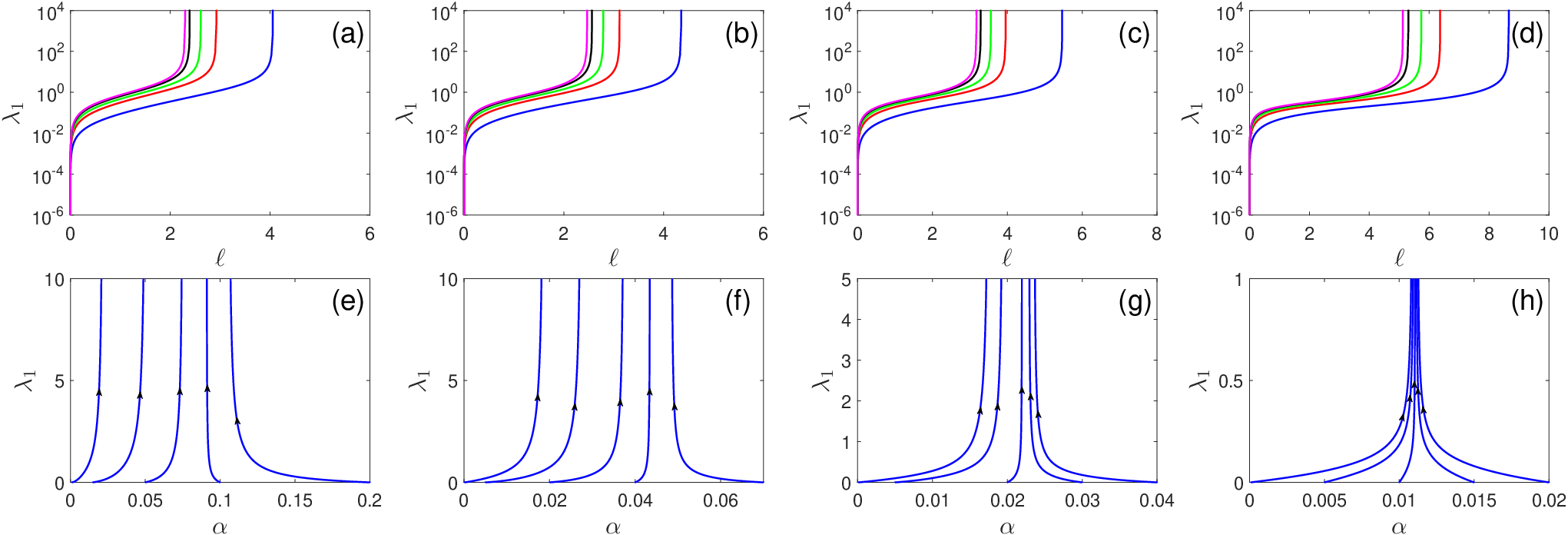
d​λ1d​ℓ=−16​λ1+(1−25​N)​λ12+FA​λ1+FB,\displaystyle\frac{d\lambda_{1}}{d\ell}=-\frac{1}{6}\lambda_{1}+\left(1-\frac{2}{5N}\right)\lambda_{1}^{2}+F_{A}\lambda_{1}+F_{B}, (36)

where the redefinition 5​Γ​(5/4)​Γ​(4/3)​Λ1/612​π2​Γ​(19/12)​A​B2/3​λ1→λ1\frac{5\Gamma\left(5/4\right)\Gamma\left(4/3\right)\Lambda^{1/6}}{12\pi^{2}\Gamma\left(19/12\right)\sqrt{A}B^{2/3}}\lambda_{1}\rightarrow\lambda_{1} has been employed. The factors FAF_{A} and FBF_{B} are induced by Coulomb interaction. The flows of λ1\lambda_{1} are presented in Fig. 4. We observe from Figs. 4(a) and 4(b) that, λ1​(ℓ)\lambda_{1}(\ell) develops a finite value from zero as ℓ\ell increases and λ1​(ℓ)\lambda_{1}(\ell) diverges as ℓ→ℓc\ell\rightarrow\ell_{c} with ℓc\ell_{c} being finite. The flow diagrams plotted in Figs. 4(c) and 4(d) show that this conclusion holds even when the initial value of α\alpha is arbitrarily small. As a result of the runaway flow of (ψ†​σ1​ψ)2(\psi^{{\dagger}}\sigma_{1}\psi)^{2}, the corresponding fermion bilinear acquires a finite expectation value, namely Δ1≡⟨ψ†​σ1​ψ⟩≠0\Delta_{1}\equiv\langle\psi^{{\dagger}}\sigma_{1}\psi\rangle\neq 0. The original band-touching point is split into three different points: (−(Δ1/B)1/3,0,0)\left(-\left(\Delta_{1}/B\right)^{1/3},0,0\right) and (12​(Δ1/B)1/3,±32​(Δ1/B)1/3,0)\left(\frac{1}{2}\left(\Delta_{1}/B\right)^{1/3},\pm\frac{\sqrt{3}}{2}\left(\Delta_{1}/B\right)^{1/3},0\right). One can identify Δ1\Delta_{1} as a nematic order parameter, because the positions of these points break the equivalence between xx- and yy-axis. Thus, the system enters into a nematic state. Around these three points, the fermion dispersion can be expressed as

E=±9​B2/3​Δ14/3​K⊥2+A2​Kz4,\displaystyle E=\pm\sqrt{9B^{2/3}\Delta_{1}^{4/3}K_{\bot}^{2}+A^{2}K_{z}^{4}}, (37)

which is linear along two directions and quadratic along the third. 𝐊\mathbf{K} is the momentum relative to the new touching points. Such a dispersion is the same as that of an anisotropic-WSM [29, 31], in which the Coulomb interaction is irrelevant at low energies, and the DOS, specific heat, and compressibility behave as ρ⁡(ω)∼ω3/2\rho(\omega)\sim\omega^{3/2}, Cv​(T)∼T5/2C_{v}(T)\sim T^{5/2}, and κ⁡(T)∼T3/2\kappa(T)\sim T^{3/2}, respectively. The mean value Δ1\Delta_{1} is nonzero only at low TT, and is destroyed as TT grows. Therefore, the NFL behaviors caused by Coulomb interaction are hidden at low TT by the nematic order, but re-appear at higher TT once the nematic order is destroyed by thermal fluctuation. The critical temperature TnT_{n} can be roughly estimated by Λ​e−ℓc\Lambda e^{-\ell_{c}}.

Similar to ⟨ψ†​σ1​ψ⟩\langle\psi^{{\dagger}}\sigma_{1}\psi\rangle, a nonzero Δ2≡⟨ψ†​σ2​ψ⟩\Delta_{2}\equiv\langle\psi^{{\dagger}}\sigma_{2}\psi\rangle also splits the original band-touching point into three new points, which are located at (0,−(Δ2/B)1/3,0)(0,-\left(\Delta_{2}/B\right)^{1/3},0) and (±32​(Δ2/B)1/3,12​(Δ2/B)1/3,0)(\pm\frac{\sqrt{3}}{2}\left(\Delta_{2}/B\right)^{1/3},\frac{1}{2}\left(\Delta_{2}/B\right)^{1/3},0). Thus, ⟨ψ†​σ2​ψ⟩\langle\psi^{{\dagger}}\sigma_{2}\psi\rangle also corresponds to nematic order parameter.

If Δ3≡⟨ψ†​σ3​ψ⟩≠0\Delta_{3}\equiv\langle\psi^{{\dagger}}\sigma_{3}\psi\rangle\neq 0, the parameter Δ\Delta (defined in Fig. 1) becomes finite, i.e., Δ=−Δ3\Delta=-\Delta_{3}, at the TQCP. Consequently, the transition between triple-WSM and BI becomes first-order [49], and the original TQCP is eliminated at low TT. At higher TT, thermal fluctuation forces Δ3\Delta_{3} to vanish, and the effective fermion dispersion is still E=±B2​k⊥6+A2​kz4E=\pm\sqrt{B^{2}k_{\bot}^{6}+A^{2}k_{z}^{4}}. The Coulomb interaction leads to NFL behaviors at high TT, which can be explored by measuring the observable quantities of Table 1.

If Δ0≡⟨ψ†​ψ⟩≠0\Delta_{0}\equiv\langle\psi^{{\dagger}}\psi\rangle\neq 0, the Fermi surface moves away from the band-touching point to a new level, since ⟨ψ†​ψ⟩\langle\psi^{{\dagger}}\psi\rangle plays the role of a finite chemical potential.

Refer to caption
Figure 4: Dependence of λ1\lambda_{1} on ℓ\ell for N=1N=1 is shown in (a) and for N=2N=2 in (b). Flow diagram on α\alpha-λ1\lambda_{1} plane for N=1N=1 is shown in (c) and for N=2N=2 in (d). Here, β0=0.1\beta_{0}=0.1.

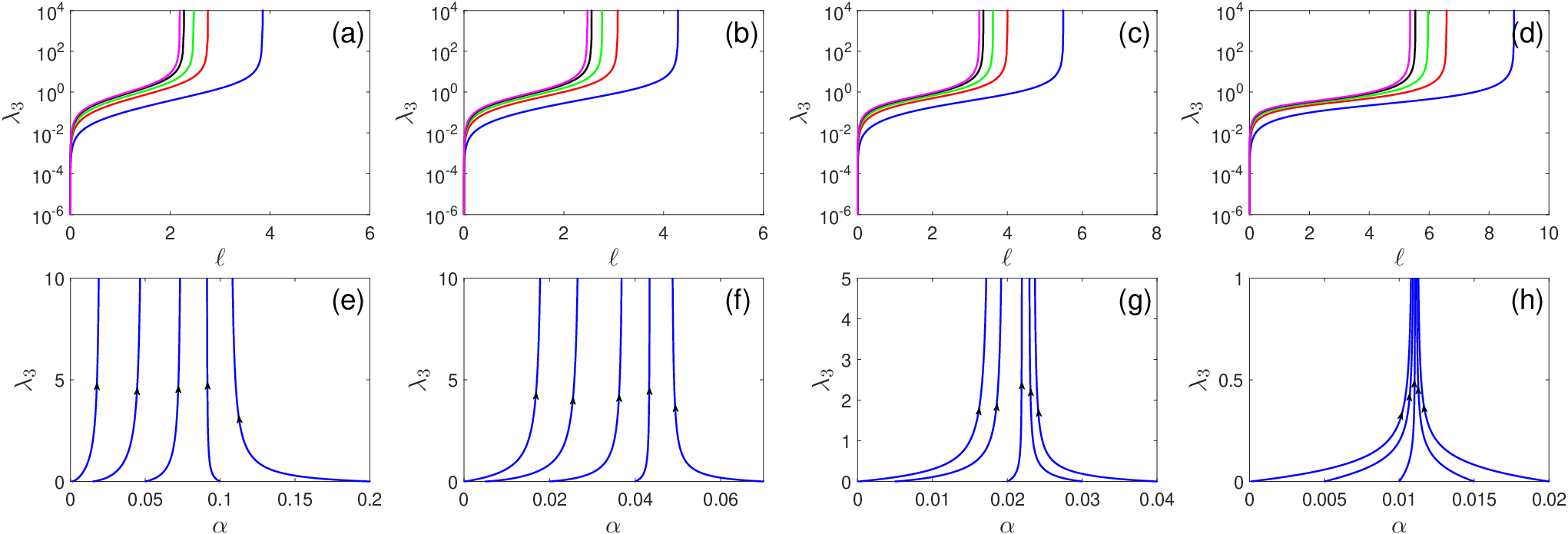
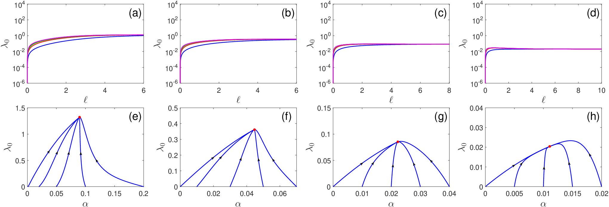
As demonstrated in Appendix F, λ2\lambda_{2} and λ3\lambda_{3} are both generated from zero, and both diverge at some finite energy scale. However, λ0\lambda_{0} grows from zero and finally approaches to a constant in the lowest energy limit, which means that Δ0≡0\Delta_{0}\equiv 0. Therefore, there are only two different instabilities, namely the formation of nematicity and the occurrence of first-order TQPT. The instability that would shift the Fermi level is excluded.

A natural question arises as to which out of the two instabilities is more favorable. As shown in Appendix F, our numerical studies reveal that, within a wide range of the initial value of α\alpha, λ3\lambda_{3} diverges most rapidly for N=1,2N=1,2, whereas λ1\lambda_{1} and λ2\lambda_{2} diverge more quickly than λ3\lambda_{3} if N≥3N\geq 3. We thus conclude that, first-order TQPT occurs for N=1,2N=1,2, but gapless nematic state is realized for N≥3N\geq 3.

VI Summary and discussion

In summary, we have investigated the quantum critical phenomena of the TQCP between the topological triple-WSM and the normal BI, and found that the long-range Coulomb interaction leads to a NFL infrared fixed point. This infrared fixed point can be experimentally probed by measuring the energy or temperature dependence of a number of observable quantities. We also have considered the interplay between Coulomb interaction and short-range interactions. Such an interplay can either causes a long-range nematic order or drive a first-order transition, depending on the value of the fermion flavor at TQCP. Comparing to some previously studied TQCPs [23, 31, 24, 25], this topological transition exhibits richer critical phenomena and provides interesting insight on the strong correlation effects at the topology-changing phase transitions.

Recent theoretical studies [30, 58, 59] predicted the presence of 3D cubic DSM state, in which the fermions have the same dispersion as triple-Weyl fermions. When a 3D cubic DSM is tuned to become a BI, the TQCP would exhibit the unusual properties predicted in this paper. It is proposed that 3D cubic-DSM can be realized in Rb(MoTe)3 and Ti(MoTe)3 [58], and LiOsO3 [59]. More candidate materials of triple-WSM or cubic-DSM might be discovered in the future. If such materials are prepared with high quality, one can tune them to approach the TQCP. We expect experiments would be performed to measure the observable quantities studied in this paper and to determine the nature of the low-energy instability. Quantum Monte Carlo simulations [60, 61, 62, 63] may help address these issues.

Note Added - After we received the referees’ reports, we had become aware of two preprints [64, 65], which study the influence of Coulomb interaction at the TQCP between double-WSM and BI.

ACKNOWLEDGEMENTS

We acknowledge the support from the National Key R&D Program of China under Grants 2016YFA0300404 and 2017YFA0403600, and that from the National Natural Science Foundation of China under Grants 11574285, 11504379, 11674327, U1532267, and U1832209.

Appendix A Self-energy of Fermion

The fermion self-energy is defined as

Σ⁡(i​ω,𝐤)\displaystyle\Sigma(i\omega,\mathbf{k}) =\displaystyle= g2​∫′d​Ω2​π​d3​𝐪(2​π)3​G0​(i​ω+i​Ω,𝐤+𝐪)\displaystyle g^{2}\int^{\prime}\frac{d\Omega}{2\pi}\frac{d^{3}\mathbf{q}}{(2\pi)^{3}}G_{0}\left(i\omega+i\Omega,\mathbf{k}+\mathbf{q}\right) (38)
×D0​(i​Ω,𝐪),\displaystyle\times D_{0}(i\Omega,\mathbf{q}),

where the free fermion propagator is

G0​(i​ω,𝐤)=1i​ω−ℋf​(𝐤),\displaystyle G_{0}(i\omega,\mathbf{k})=\frac{1}{i\omega-\mathcal{H}_{f}(\mathbf{k})}, (39)

where

ℋf​(𝐤)=B⁡[d1​(𝐤)​σ1+d2​(𝐤)​σ2]+A​d3​(𝐤)​σ3,\displaystyle\mathcal{H}_{f}(\mathbf{k})=B[d_{1}(\mathbf{k})\sigma_{1}+d_{2}(\mathbf{k})\sigma_{2}]+Ad_{3}(\mathbf{k})\sigma_{3}, (40)

with d1​(𝐤)=(kx3−3​kx​ky2)d_{1}(\mathbf{k})=\left(k_{x}^{3}-3k_{x}k_{y}^{2}\right), d2​(𝐤)=(ky3−3​ky​kx2)d_{2}(\mathbf{k})=\left(k_{y}^{3}-3k_{y}k_{x}^{2}\right), and d3​(𝐤)=kz2d_{3}(\mathbf{k})=k_{z}^{2}. The free boson propagator is given by

D0​(i​Ω,𝐪)=D0​(𝐪)=1qx2+qy2+η​qz2=1q⊥2+η​qz2.\displaystyle D_{0}(i\Omega,\mathbf{q})=D_{0}(\mathbf{q})=\frac{1}{q_{x}^{2}+q_{y}^{2}+\eta q_{z}^{2}}=\frac{1}{q_{\bot}^{2}+\eta q_{z}^{2}}. (41)

Substituting Eqs. (39) and (41) into Eq. (38), and retaining the leading order of contribution, we obtain

Σ⁡(i​ω,𝐤)\displaystyle\Sigma(i\omega,\mathbf{k}) ≈\displaystyle\approx i​ω​Σ1−B⁡[d1​(𝐤)​σ1+d2​(𝐤)​σ2]​Σ2\displaystyle i\omega\Sigma_{1}-B\left[d_{1}(\mathbf{k})\sigma_{1}+d_{2}(\mathbf{k})\sigma_{2}\right]\Sigma_{2} (42)
−A​d3​(𝐤)​σ3​Σ3,\displaystyle-Ad_{3}(\mathbf{k})\sigma_{3}\Sigma_{3},

where

Σ1\displaystyle\Sigma_{1} =\displaystyle= g24​π3​∫′d​Ω​d​q⊥​d​|qz|​q⊥​Ω2−B2​q⊥6−A2​qz4(Ω2+B2​q⊥6+A2​qz4)2\displaystyle\frac{g^{2}}{4\pi^{3}}\int^{\prime}d\Omega dq_{\bot}d|q_{z}|q_{\bot}\frac{\Omega^{2}-B^{2}q_{\bot}^{6}-A^{2}q_{z}^{4}}{\left(\Omega^{2}+B^{2}q_{\bot}^{6}+A^{2}q_{z}^{4}\right)^{2}} (43)
×D0​(i​Ω,𝐪),\displaystyle\times D_{0}(i\Omega,\mathbf{q}),
Σ2\displaystyle\Sigma_{2} =\displaystyle= g24​π3∫′dΩdq⊥d|qz|q⊥[Ω2−18​B2​q⊥6+A2​qz4(Ω2+B2​q⊥6+A2​qz4)2\displaystyle\frac{g^{2}}{4\pi^{3}}\int^{\prime}d\Omega dq_{\bot}d|q_{z}|q_{\bot}\left[\frac{\Omega^{2}-18B^{2}q_{\bot}^{6}+A^{2}q_{z}^{4}}{\left(\Omega^{2}+B^{2}q_{\bot}^{6}+A^{2}q_{z}^{4}\right)^{2}}\right. (44)
+45​B4​q⊥12(Ω2+B2​q⊥6+A2​qz4)3\displaystyle+\frac{45B^{4}q_{\bot}^{12}}{\left(\Omega^{2}+B^{2}q_{\bot}^{6}+A^{2}q_{z}^{4}\right)^{3}}
−27​B6​q⊥18(Ω2+B2​q⊥6+A2​qz4)4]D0(iΩ,𝐪),\displaystyle\left.-\frac{27B^{6}q_{\bot}^{18}}{\left(\Omega^{2}+B^{2}q_{\bot}^{6}+A^{2}q_{z}^{4}\right)^{4}}\right]D_{0}(i\Omega,\mathbf{q}),
Σ3\displaystyle\Sigma_{3} =\displaystyle= g24​π3∫′dΩdq⊥d|qz|q⊥[Ω2+B2​q⊥6−13​A2​qz4(Ω2+B2​q⊥6+A2​qz4)2\displaystyle\frac{g^{2}}{4\pi^{3}}\int^{\prime}d\Omega dq_{\bot}d|q_{z}|q_{\bot}\left[\frac{\Omega^{2}+B^{2}q_{\bot}^{6}-13A^{2}q_{z}^{4}}{\left(\Omega^{2}+B^{2}q_{\bot}^{6}+A^{2}q_{z}^{4}\right)^{2}}\right. (45)
+16​A4​qz8(Ω2+B2​q⊥6+A2​qz4)3]D0(iΩ,𝐪).\displaystyle\left.+\frac{16A^{4}q_{z}^{8}}{\left(\Omega^{2}+B^{2}q_{\bot}^{6}+A^{2}q_{z}^{4}\right)^{3}}\right]D_{0}(i\Omega,\mathbf{q}).

In the following, we will employ the transformations

E=B2​q⊥6+A2​qz4,ξ=B​q⊥3A​|qz|2,\displaystyle E=\sqrt{B^{2}q_{\bot}^{6}+A^{2}q_{z}^{4}},\qquad\xi=\frac{Bq_{\bot}^{3}}{A\left|q_{z}\right|^{2}}, (46)

which are equivalent to

q⊥=ξ1/3​E1/3B1/3​(1+ξ2)1/6,|qz|=EA​(1+ξ2)1/4.\displaystyle q_{\bot}=\frac{\xi^{1/3}E^{1/3}}{B^{1/3}\left(1+\xi^{2}\right)^{1/6}},\quad|q_{z}|=\frac{\sqrt{E}}{\sqrt{A}\left(1+\xi^{2}\right)^{1/4}}. (47)

The measures of the integrations satisfy the relation

d​q⊥​d​|qz|\displaystyle dq_{\bot}d|q_{z}| =\displaystyle= ||∂q⊥∂E∂q⊥∂ξ∂|qz|∂E∂|qz|∂ξ||​d​E​d​ξ\displaystyle\left|\left|\begin{array}[]{cc}\frac{\partial q_{\bot}}{\partial E}&\frac{\partial q_{\bot}}{\partial\xi}\\ \frac{\partial|q_{z}|}{\partial E}&\frac{\partial|q_{z}|}{\partial\xi}\end{array}\right|\right|dEd\xi (51)
=\displaystyle= |∂q⊥∂E​∂|qz|∂ξ−∂q⊥∂ξ​∂|qz|∂E|​d​E​d​ξ\displaystyle\left|\frac{\partial q_{\bot}}{\partial E}\frac{\partial|q_{z}|}{\partial\xi}-\frac{\partial q_{\bot}}{\partial\xi}\frac{\partial|q_{z}|}{\partial E}\right|dEd\xi
=\displaystyle= d​E​d​ξ6​A​B1/3​E1/6​ξ2/3​(1+ξ2)5/12.\displaystyle\frac{dEd\xi}{6\sqrt{A}B^{1/3}E^{1/6}\xi^{2/3}\left(1+\xi^{2}\right)^{5/12}}.

To proceed with RG calculations, we choose to integrate out high-energy modes defined in the momentum shell

−∞<Ω<∞,b​Λ<E<Λ,\displaystyle-\infty<\Omega<\infty,\qquad b\Lambda<E<\Lambda, (52)

with E=B2​q⊥6+A2​qz4E=\sqrt{B^{2}q_{\bot}^{6}+A^{2}q_{z}^{4}} and b=e−ℓb=e^{-\ell}. Utilizing the transformations Eqs. (46)-(51), we obtain

Σ⁡(i​ω,𝐤)\displaystyle\Sigma(i\omega,\mathbf{k}) ≈\displaystyle\approx −B⁡[d1​(𝐤)​σ1+d2​(𝐤)​σ2]​C2​ℓ\displaystyle-B\left[d_{1}(\mathbf{k})\sigma_{1}+d_{2}(\mathbf{k})\sigma_{2}\right]C_{2}\ell (53)
−A​d3​(𝐤)​σ3​C3​ℓ,\displaystyle-Ad_{3}(\mathbf{k})\sigma_{3}C_{3}\ell,

where

C2\displaystyle C_{2} =\displaystyle= g248​π2​A​Λ​∫0+∞d​ξ​1ξ1/3​(1+ξ2)13/12\displaystyle\frac{g^{2}}{48\pi^{2}\sqrt{A\Lambda}}\int_{0}^{+\infty}d\xi\frac{1}{\xi^{1/3}\left(1+\xi^{2}\right)^{13/12}} (54)
×[2−17​ξ2+1354​ξ4(1+ξ2)−1358​ξ6(1+ξ2)2]\displaystyle\times\left[2-17\xi^{2}+\frac{135}{4}\frac{\xi^{4}}{\left(1+\xi^{2}\right)}-\frac{135}{8}\frac{\xi^{6}}{\left(1+\xi^{2}\right)^{2}}\right]
×1ξ2/3​(1+ξ2)1/6+ζ,\displaystyle\times\frac{1}{\xi^{2/3}\left(1+\xi^{2}\right)^{1/6}+\zeta},
C3\displaystyle C_{3} =\displaystyle= g224​π2​A​Λ​∫0+∞d​ξ​1ξ1/3​(1+ξ2)13/12\displaystyle\frac{g^{2}}{24\pi^{2}\sqrt{A\Lambda}}\int_{0}^{+\infty}d\xi\frac{1}{\xi^{1/3}\left(1+\xi^{2}\right)^{13/12}} (55)
×(ξ2−6+61+ξ2)​1ξ2/3​(1+ξ2)1/6+ζ,\displaystyle\times\left(\xi^{2}-6+\frac{6}{1+\xi^{2}}\right)\frac{1}{\xi^{2/3}\left(1+\xi^{2}\right)^{1/6}+\zeta},

with ζ=η​B2/3​Λ1/3A\zeta=\frac{\eta B^{2/3}\Lambda^{1/3}}{A}.

Appendix B Self-energy of Boson

The boson self-energy is given by

Π⁡(i​Ω,𝐪)\displaystyle\Pi(i\Omega,\mathbf{q}) =\displaystyle= −Ng2∫d​ω2​π∫′d3​𝐤(2​π)3Tr[G0(iω,𝐤)\displaystyle-Ng^{2}\int\frac{d\omega}{2\pi}\int^{\prime}\frac{d^{3}\mathbf{k}}{(2\pi)^{3}}\mathrm{Tr}\left[G_{0}(i\omega,\mathbf{k})\right. (56)
×G0(iω+iΩ,𝐤+𝐪)].\displaystyle\left.\times G_{0}\left(i\omega+i\Omega,\mathbf{k}+\mathbf{q}\right)\right].

Substituting Eq. (39) into Eq. (56), Π⁡(i​Ω,𝐪)\Pi(i\Omega,\mathbf{q}) can be further written as

Π⁡(i​Ω,𝐪)\displaystyle\Pi(i\Omega,\mathbf{q}) =\displaystyle= 2​N​g2​∫−∞+∞d​ω2​π​∫′d3​𝐤(2​π)3\displaystyle 2Ng^{2}\int_{-\infty}^{+\infty}\frac{d\omega}{2\pi}\int^{\prime}\frac{d^{3}\mathbf{k}}{(2\pi)^{3}} (57)
×1(ω2+E𝐤2)​[(ω+Ω)2+E𝐤+𝐪2]{ω(ω+Ω)\displaystyle\times\frac{1}{\left(\omega^{2}+E_{\mathbf{k}}^{2}\right)\left[(\omega+\Omega)^{2}+E_{\mathbf{k}+\mathbf{q}}^{2}\right]}\big\{\omega(\omega+\Omega)
−B2​[d1​(𝐤)​d1​(𝐤+𝐪)+d2​(𝐤)​d2​(𝐤+𝐪)]\displaystyle-B^{2}\left[d_{1}(\mathbf{k})d_{1}(\mathbf{k}+\mathbf{q})+d_{2}(\mathbf{k})d_{2}(\mathbf{k}+\mathbf{q})\right]
−A2d3(𝐤)d3(𝐤+𝐪)},\displaystyle-A^{2}d_{3}(\mathbf{k})d_{3}(\mathbf{k}+\mathbf{q})\big\},

where E𝐤=B2​k⊥6+A2​kz4E_{\mathbf{k}}=\sqrt{B^{2}k_{\bot}^{6}+A^{2}k_{z}^{4}}. Taking the static limit Ω=0\Omega=0, and then expanding to the leading order of q⊥q_{\bot} and qzq_{z}, we get

Π⁡(0,𝐪)\displaystyle\Pi(0,\mathbf{q}) ≈\displaystyle\approx q⊥2​N​9​g216​π2​∫′d​k⊥​d​|kz|​k⊥​(2​B2​k⊥4E𝐤3−B4​k⊥10E𝐤5)\displaystyle q_{\bot}^{2}N\frac{9g^{2}}{16\pi^{2}}\int^{\prime}dk_{\bot}d|k_{z}|k_{\bot}\left(\frac{2B^{2}k_{\bot}^{4}}{E_{\mathbf{k}}^{3}}-\frac{B^{4}k_{\bot}^{10}}{E_{\mathbf{k}}^{5}}\right) (58)
+qz2Ng22​π2∫′dk⊥d|kz|k⊥A2​kz2​B2​k⊥6E𝐤5.\displaystyle+q_{z}^{2}N\frac{g^{2}}{2\pi^{2}}\int^{\prime}dk_{\bot}d|k_{z}|k_{\bot}\frac{A^{2}k_{z}^{2}B^{2}k_{\bot}^{6}}{E_{\mathbf{k}}^{5}}.

Using again the transformations Eqs. (46)-(51), we finally obtain

Π⁡(0,𝐪)\displaystyle\Pi(0,\mathbf{q}) ≈\displaystyle\approx q⊥2​N​C⊥​ℓ+qz2​N​Cz​ℓ,\displaystyle q_{\bot}^{2}NC_{\bot}\ell+q_{z}^{2}NC_{z}\ell,

where

C⊥=9​g240​π2​A​Λ,Cz=Γ⁡(34)​Γ​(43)​g2​A24​π2​Γ​(2512)​B2/3​Λ5/6.\displaystyle C_{\bot}=\frac{9g^{2}}{40\pi^{2}\sqrt{A\Lambda}},\quad C_{z}=\frac{\Gamma\left(\frac{3}{4}\right)\Gamma\left(\frac{4}{3}\right)g^{2}\sqrt{A}}{24\pi^{2}\Gamma\left(\frac{25}{12}\right)B^{2/3}\Lambda^{5/6}}. (59)

Appendix C Derivation of RG equations

The free action of fermion field ψ\psi is

Sψ\displaystyle S_{\psi} =\displaystyle= ∫d​ω2​πd3​𝐤(2​π)3ψa†(ω,𝐤){iω−B[d1(𝐤)σ1+d2(𝐤)σ2]\displaystyle\int\frac{d\omega}{2\pi}\frac{d^{3}\mathbf{k}}{(2\pi)^{3}}\psi_{a}^{{\dagger}}(\omega,\mathbf{k})\left\{i\omega-B[d_{1}(\mathbf{k})\sigma_{1}+d_{2}(\mathbf{k})\sigma_{2}]\right. (60)
−Ad3(𝐤)σ3}ψa(ω,𝐤).\displaystyle\left.-Ad_{3}(\mathbf{k})\sigma_{3}\right\}\psi_{a}(\omega,\mathbf{k}).

Upon incorporating the interaction corrections, we get

Sψ\displaystyle S_{\psi} =\displaystyle= ∫d​ω2​πd3​𝐤(2​π)3ψa†(ω,𝐤){iω−B[d1(𝐤)σ1+d2(𝐤)σ2]\displaystyle\int\frac{d\omega}{2\pi}\frac{d^{3}\mathbf{k}}{(2\pi)^{3}}\psi_{a}^{{\dagger}}(\omega,\mathbf{k})\left\{i\omega-B[d_{1}(\mathbf{k})\sigma_{1}+d_{2}(\mathbf{k})\sigma_{2}]\right. (61)
−Ad3(𝐤)σ3+Σ(iω,𝐤)}ψa(ω,𝐤)\displaystyle\left.-Ad_{3}(\mathbf{k})\sigma_{3}+\Sigma(i\omega,\mathbf{k})\right\}\psi_{a}(\omega,\mathbf{k})
≈\displaystyle\approx ∫d​ω2​πd3​𝐤(2​π)3ψa†(ω,𝐤){iω−B[d1(𝐤)σ1+d2(𝐤)σ2]\displaystyle\int\frac{d\omega}{2\pi}\frac{d^{3}\mathbf{k}}{(2\pi)^{3}}\psi_{a}^{{\dagger}}(\omega,\mathbf{k})\Big\{i\omega-B\left[d_{1}(\mathbf{k})\sigma_{1}+d_{2}(\mathbf{k})\sigma_{2}\right]
×eC2​ℓ−Ad3(𝐤)σ3eC3​ℓ}ψa(ω,𝐤).\displaystyle\times e^{C_{2}\ell}-Ad_{3}(\mathbf{k})\sigma_{3}e^{C_{3}\ell}\Big\}\psi_{a}(\omega,\mathbf{k}).

Using the re-scaling transformations

ω\displaystyle\omega =\displaystyle= ω′​e−ℓ,\displaystyle\omega^{\prime}e^{-\ell}, (62)
kx\displaystyle k_{x} =\displaystyle= kx′​e−ℓ3,\displaystyle k_{x}^{\prime}e^{-\frac{\ell}{3}}, (63)
ky\displaystyle k_{y} =\displaystyle= ky′​e−ℓ3,\displaystyle k_{y}^{\prime}e^{-\frac{\ell}{3}}, (64)
kz\displaystyle k_{z} =\displaystyle= kz′​e−ℓ2,\displaystyle k_{z}^{\prime}e^{-\frac{\ell}{2}}, (65)
ψa\displaystyle\psi_{a} =\displaystyle= ψa′​e1912​ℓ,\displaystyle\psi_{a}^{\prime}e^{\frac{19}{12}\ell}, (66)
B\displaystyle B =\displaystyle= B′​e−C2​ℓ,\displaystyle B^{\prime}e^{-C_{2}\ell}, (67)
A\displaystyle A =\displaystyle= A′​e−C3​ℓ,\displaystyle A^{\prime}e^{-C_{3}\ell}, (68)

the action can be re-written as

Sψ′\displaystyle S_{\psi^{\prime}} =\displaystyle= ∫d​ω′2​πd3​𝐤′(2​π)3ψ′a†(ω′,𝐤′){iω′−B′[d1(𝐤′)σ1\displaystyle\int\frac{d\omega^{\prime}}{2\pi}\frac{d^{3}\mathbf{k}^{\prime}}{(2\pi)^{3}}{\psi^{\prime}}_{a}^{{\dagger}}(\omega^{\prime},\mathbf{k^{\prime}})\big\{i\omega^{\prime}-B^{\prime}\left[d_{1}(\mathbf{k}^{\prime})\sigma_{1}\right. (69)
+d2(𝐤′)σ2]−A′d3(𝐤′)σ3}ψa′(ω′,𝐤′),\displaystyle\left.+d_{2}(\mathbf{k}^{\prime})\sigma_{2}\right]-A^{\prime}d_{3}(\mathbf{k}^{\prime})\sigma_{3}\big\}\psi_{a}^{\prime}(\omega^{\prime},\mathbf{k}^{\prime}),

which recovers the original form of the action.

The free action of boson field ϕ\phi takes the form

Sϕ=∫d​ω2​π​d3​𝐤(2​π)3​ϕ​(ω,𝐤)​(k⊥2+η​kz2)​ϕ​(ω,𝐤).\displaystyle S_{\phi}=\int\frac{d\omega}{2\pi}\frac{d^{3}\mathbf{k}}{(2\pi)^{3}}\phi(\omega,\mathbf{k})\left(k_{\bot}^{2}+\eta k_{z}^{2}\right)\phi(\omega,\mathbf{k}). (70)

Including the interaction correction converts the action ϕ\phi to

Sϕ\displaystyle S_{\phi} =\displaystyle= ∫d​ω2​π​d3​𝐤(2​π)3​ϕ​(ω,𝐤)​[k⊥2+η​kz2+Π⁡(0,𝐤)]​ϕ​(ω,𝐤)\displaystyle\int\frac{d\omega}{2\pi}\frac{d^{3}\mathbf{k}}{(2\pi)^{3}}\phi(\omega,\mathbf{k})\left[k_{\bot}^{2}+\eta k_{z}^{2}+\Pi(0,\mathbf{k})\right]\phi(\omega,\mathbf{k}) (71)
≈\displaystyle\approx ∫d​ω2​π​d3​𝐤(2​π)3​ϕ​(ω,𝐤)​[k⊥2​eN​C⊥​ℓ+(η+N​Cz​ℓ)​kz2]\displaystyle\int\frac{d\omega}{2\pi}\frac{d^{3}\mathbf{k}}{(2\pi)^{3}}\phi(\omega,\mathbf{k})\left[k_{\bot}^{2}e^{NC_{\bot}\ell}+\left(\eta+NC_{z}\ell\right)k_{z}^{2}\right]
×ϕ⁡(ω,𝐤).\displaystyle\times\phi(\omega,\mathbf{k}).

Making use of the transformations Eqs. (62)-(65), we find that the field ϕ\phi should be re-scaled as follows

ϕ=ϕ′​e−12​(−176+N​C⊥)​ℓ.\displaystyle\phi=\phi^{\prime}e^{-\frac{1}{2}\left(-\frac{17}{6}+NC_{\bot}\right)\ell}. (72)

Now the action of ϕ′\phi^{\prime} can be approximately written as

Sϕ′\displaystyle S_{\phi^{\prime}} ≈\displaystyle\approx ∫d​ω′2​πd3​𝐤′(2​π)3ϕ′(ω′,𝐤′){k⊥′2+[η−η(13+NC⊥)\displaystyle\int\frac{d\omega^{\prime}}{2\pi}\frac{d^{3}\mathbf{k}^{\prime}}{(2\pi)^{3}}\phi^{\prime}(\omega^{\prime},\mathbf{k}^{\prime})\bigg\{k_{\bot}^{\prime 2}+\Big[\eta-\eta\Big(\frac{1}{3}+NC_{\bot}\Big) (73)
×ℓ+NCzℓ]kz′2}ϕ′(ω′,𝐤′).\displaystyle\times\ell+NC_{z}\ell\Big]k_{z}^{\prime 2}\bigg\}\phi^{\prime}(\omega^{\prime},\mathbf{k}^{\prime}).

We define

η′=η−η⁡(13+N​C⊥)​ℓ+N​Cz​ℓ,\displaystyle\eta^{\prime}=\eta-\eta\left(\frac{1}{3}+NC_{\bot}\right)\ell+NC_{z}\ell, (74)

and then get

Sϕ′\displaystyle S_{\phi^{\prime}} =\displaystyle= ∫d​ω′2​π​d3​𝐤′(2​π)3​ϕ′​(ω′,𝐤′)​(k⊥′2+η′​kz′2)\displaystyle\int\frac{d\omega^{\prime}}{2\pi}\frac{d^{3}\mathbf{k}^{\prime}}{(2\pi)^{3}}\phi^{\prime}(\omega^{\prime},\mathbf{k}^{\prime})\left(k_{\bot}^{\prime 2}+\eta^{\prime}k_{z}^{\prime 2}\right) (75)
×ϕ′​(ω′,𝐤′),\displaystyle\times\phi^{\prime}(\omega^{\prime},\mathbf{k}^{\prime}),

which has the same form as the original boson action.

Refer to caption
Figure 5: (a)-(h): Flow diagrams on the α\alpha-β\beta plane at N=1,2,3,4,5,6,7,8N=1,2,3,4,5,6,7,8, respectively.

The action of fermion-boson coupling is

Sψ​ϕ\displaystyle S_{\psi\phi} =\displaystyle= g​∫d​ω12​π​d3​𝐤1(2​π)3​d​ω22​π​d3​𝐤2(2​π)3​ψa†​(ω1,𝐤1)​ψa​(ω2,𝐤2)\displaystyle g\int\frac{d\omega_{1}}{2\pi}\frac{d^{3}\mathbf{k}_{1}}{(2\pi)^{3}}\frac{d\omega_{2}}{2\pi}\frac{d^{3}\mathbf{k}_{2}}{(2\pi)^{3}}\psi_{a}^{{\dagger}}(\omega_{1},\mathbf{k}_{1})\psi_{a}(\omega_{2},\mathbf{k}_{2}) (76)
×ϕ⁡(ω1−ω2,𝐤1−𝐤2).\displaystyle\times\phi(\omega_{1}-\omega_{2},\mathbf{k}_{1}-\mathbf{k}_{2}).

Making use of the transformations Eqs. (62)-(66) and (72), we find that

Sψ′​ϕ′\displaystyle S_{\psi^{\prime}\phi^{\prime}} =\displaystyle= g​e(14−N​C⊥2)​ℓ​∫d​ω1′2​π​d3​𝐤1′(2​π)3​d​ω2′2​π​d3​𝐤2′(2​π)3​ψa′⁣†​(ω1′,𝐤1′)\displaystyle ge^{\left(\frac{1}{4}-\frac{NC_{\bot}}{2}\right)\ell}\int\frac{d\omega_{1}^{\prime}}{2\pi}\frac{d^{3}\mathbf{k}_{1}^{\prime}}{(2\pi)^{3}}\frac{d\omega_{2}^{\prime}}{2\pi}\frac{d^{3}\mathbf{k}_{2}^{\prime}}{(2\pi)^{3}}\psi^{\prime{\dagger}}_{a}(\omega_{1}^{\prime},\mathbf{k}_{1}^{\prime}) (77)
×ψa′​(ω2′,𝐤2′)​ϕ′​(ω1′−ω2′,𝐤1′−𝐤2).\displaystyle\times\psi^{\prime}_{a}(\omega_{2}^{\prime},\mathbf{k}_{2}^{\prime})\phi^{\prime}(\omega_{1}^{\prime}-\omega_{2}^{\prime},\mathbf{k}_{1}^{\prime}-\mathbf{k}_{2}).

Adopting the re-scaling transformation

g′=g​e(14−N​C⊥2)​ℓ,\displaystyle g^{\prime}=ge^{\left(\frac{1}{4}-\frac{NC_{\bot}}{2}\right)\ell}, (78)

we further re-write the action in the form

Sψ′​ϕ′\displaystyle S_{\psi^{\prime}\phi^{\prime}} =\displaystyle= g′​∫d​ω1′2​π​d3​𝐤1′(2​π)3​d​ω2′2​π​d3​𝐤2′(2​π)3​ψa′⁣†​(ω1′,𝐤1′)\displaystyle g^{\prime}\int\frac{d\omega_{1}^{\prime}}{2\pi}\frac{d^{3}\mathbf{k}_{1}^{\prime}}{(2\pi)^{3}}\frac{d\omega_{2}^{\prime}}{2\pi}\frac{d^{3}\mathbf{k}_{2}^{\prime}}{(2\pi)^{3}}\psi^{\prime{\dagger}}_{a}(\omega_{1}^{\prime},\mathbf{k}_{1}^{\prime}) (79)
×ψa′​(ω2′,𝐤2′)​ϕa′​(ω1′−ω2′,𝐤1′−𝐤2′),\displaystyle\times\psi^{\prime}_{a}(\omega_{2}^{\prime},\mathbf{k}_{2}^{\prime})\phi^{\prime}_{a}(\omega_{1}^{\prime}-\omega_{2}^{\prime},\mathbf{k}_{1}^{\prime}-\mathbf{k}_{2}^{\prime}),

which recovers the form of the original interacting action.

From the transformations given by Eqs. (67), (68), (74), and (78), we obtain the following RG equations

d​Bd​ℓ\displaystyle\frac{dB}{d\ell} =\displaystyle= C2​B,\displaystyle C_{2}B, (80)
d​Ad​ℓ\displaystyle\frac{dA}{d\ell} =\displaystyle= C3​A,\displaystyle C_{3}A, (81)
d​αd​ℓ\displaystyle\frac{d\alpha}{d\ell} =\displaystyle= (12−N​C⊥−C32)​α,\displaystyle\left(\frac{1}{2}-NC_{\bot}-\frac{C_{3}}{2}\right)\alpha, (82)
d​βd​ℓ\displaystyle\frac{d\beta}{d\ell} =\displaystyle= (56+12​C3−23​C2−N​β)​β,\displaystyle\left(\frac{5}{6}+\frac{1}{2}C_{3}-\frac{2}{3}C_{2}-N\beta\right)\beta, (83)
d​ηd​ℓ\displaystyle\frac{d\eta}{d\ell} =\displaystyle= (−13−N​C⊥+N​β)​η,\displaystyle\left(-\frac{1}{3}-NC_{\bot}+N\beta\right)\eta, (84)
d​ζd​ℓ\displaystyle\frac{d\zeta}{d\ell} =\displaystyle= (−13+23​C2−C3−N​C⊥+N​β)​ζ,\displaystyle\left(-\frac{1}{3}+\frac{2}{3}C_{2}-C_{3}-NC_{\bot}+N\beta\right)\zeta, (85)

where α\alpha and β\beta are defined as

α\displaystyle\alpha =\displaystyle= g28​π3​A​Λ,\displaystyle\frac{g^{2}}{8\pi^{3}\sqrt{A\Lambda}}, (86)
β\displaystyle\beta =\displaystyle= Czη=Γ⁡(34)​Γ​(43)​g2​A24​π2​Γ​(2512)​B2/3​Λ5/6​η.\displaystyle\frac{C_{z}}{\eta}=\frac{\Gamma\left(\frac{3}{4}\right)\Gamma\left(\frac{4}{3}\right)g^{2}\sqrt{A}}{24\pi^{2}\Gamma\left(\frac{25}{12}\right)B^{2/3}\Lambda^{5/6}\eta}. (87)

As shown in Fig. 5, (α\alpha,β\beta) always flows to a stable fixed point (α∗,β∗)(\alpha^{*},\beta^{*}). The concrete values of α∗\alpha^{*} and β∗\beta^{*} are determined by the fermion flavor NN. The values of α∗\alpha^{*}, β∗\beta^{*}, and several other parameters obtained for different fermion flavors are summarized in Table 2.

Table 2: Dependence of the parameters α∗\alpha^{*}, β∗\beta^{*}, C2∗C_{2}^{*}, C3∗C_{3}^{*}, C⊥∗C_{\bot}^{*}, N​α∗N\alpha^{*}, N​β∗N\beta^{*}, N​C⊥∗NC_{\bot}^{*} on NN at the stable fixed point.
NN α∗\alpha^{*} β∗\beta^{*} C2∗C_{2}^{*} C3∗C_{3}^{*} C⊥∗C_{\bot}^{*} N​α∗N\alpha^{*} N​β∗N\beta^{*} N​C⊥∗NC_{\bot}^{*}
1 0.08997 0.7364 0.1322 -0.01754 0.5088 0.08997 0.7364 0.5088
2 0.04462 0.3914 0.06891 -0.009236 0.2523 0.08924 0.7828 0.5046
3 0.02966 0.2664 0.04567 -0.006258 0.1677 0.08897 0.7992 0.5031
4 0.02221 0.2019 0.03517 -0.004731 0.1256 0.08884 0.8075 0.5024
5 0.01775 0.1625 0.02825 -0.003802 0.1004 0.08876 0.8126 0.5019
6 0.01478 0.1360 0.02361 -0.003178 0.08360 0.08870 0.8160 0.5016
7 0.01267 0.1169 0.02027 -0.002730 0.07162 0.08866 0.8185 0.5014
8 0.01108 0.1025 0.01776 -0.002393 0.06265 0.08863 0.8203 0.5012
9 0.009845 0.09130 0.01581 -0.002130 0.05567 0.08861 0.8217 0.5010
10 0.008859 0.08229 0.01424 -0.001919 0.05010 0.08859 0.8229 0.5010

Appendix D Observable quantities in the free case

Here, we will calculate a number of observable quantities, first in the non-interacting limit.

D.1 Density of states

The retarded fermion propagator takes the form

G0ret​(ω,𝐤)=1ω−ℋf​(𝐤)+i​δ.\displaystyle G_{0}^{\mathrm{ret}}(\omega,\mathbf{k})=\frac{1}{\omega-\mathcal{H}_{f}(\mathbf{k})+i\delta}. (88)

Its imaginary part can be easily obtained:

Im⁡[G0ret​(ω,𝐤)]\displaystyle\mathrm{Im}\left[G_{0}^{\mathrm{ret}}(\omega,\mathbf{k})\right] =\displaystyle= −π​sgn​(ω)​[ω+ℋf​(𝐤)]​12​E𝐤\displaystyle-\pi\mathrm{sgn}(\omega)\left[\omega+\mathcal{H}_{f}(\mathbf{k})\right]\frac{1}{2E_{\mathbf{k}}} (89)
×[δ⁡(ω+E𝐤)+δ⁡(ω−E𝐤)].\displaystyle\times\left[\delta\left(\omega+E_{\mathbf{k}}\right)+\delta\left(\omega-E_{\mathbf{k}}\right)\right].

The spectral function is given by

𝒜⁡(ω,𝐤)\displaystyle\mathcal{A}(\omega,\mathbf{k}) =\displaystyle= −1π​Tr​[Im⁡[G0ret​(ω,𝐤)]]\displaystyle-\frac{1}{\pi}\mathrm{Tr}\left[\mathrm{Im}\left[G_{0}^{\mathrm{ret}}(\omega,\mathbf{k})\right]\right] (90)
=\displaystyle= |ω|​1E𝐤​[δ⁡(ω+E𝐤)+δ⁡(ω−E𝐤)],\displaystyle\left|\omega\right|\frac{1}{E_{\mathbf{k}}}\left[\delta\left(\omega+E_{\mathbf{k}}\right)+\delta\left(\omega-E_{\mathbf{k}}\right)\right],

which directly leads to the fermion DOS

ρ⁡(ω)\displaystyle\rho(\omega) =\displaystyle= N​∫d3​𝐤(2​π)3​𝒜​(ω,𝐤)\displaystyle N\int\frac{d^{3}\mathbf{k}}{(2\pi)^{3}}\mathcal{A}(\omega,\mathbf{k}) (91)
=\displaystyle= |ω|2​π2∫dk⊥d|kz|k⊥1E𝐤[δ(ω+E𝐤)\displaystyle\frac{|\omega|}{2\pi^{2}}\int dk_{\bot}d|k_{z}|k_{\bot}\frac{1}{E_{\mathbf{k}}}\left[\delta\left(\omega+E_{\mathbf{k}}\right)\right.
+δ(ω−E𝐤)].\displaystyle\left.+\delta\left(\omega-E_{\mathbf{k}}\right)\right].

After integrating over the momenta, we obtain

ρ⁡(ω)=N​c1A​B2/3​|ω|1/6,\displaystyle\rho(\omega)=\frac{Nc_{1}}{\sqrt{A}B^{2/3}}|\omega|^{1/6}, (92)

where

c1\displaystyle c_{1} =\displaystyle= Γ⁡(13)​Γ​(54)6​π2​Γ​(712)≈0.02682.\displaystyle\frac{\Gamma\left(\frac{1}{3}\right)\Gamma\left(\frac{5}{4}\right)}{6\pi^{2}\Gamma\left(\frac{7}{12}\right)}\approx 0.02682. (93)

D.2 Specific heat

The Matsubara fermion propagator has the form

G0​(i​ωn,𝐤)\displaystyle G_{0}(i\omega_{n},\mathbf{k}) =\displaystyle= 1i​ωn−ℋf​(𝐤)\displaystyle\frac{1}{i\omega_{n}-\mathcal{H}_{f}(\mathbf{k})} (94)
=\displaystyle= −i​ωn−ℋf​(𝐤)ωn2+E𝐤2,\displaystyle\frac{-i\omega_{n}-\mathcal{H}_{f}(\mathbf{k})}{\omega_{n}^{2}+E_{\mathbf{k}}^{2}},

where ωn=(2​n+1)​π​T\omega_{n}=(2n+1)\pi T with nn being integers. The free energy of fermions is

Ff​(T)\displaystyle F_{f}(T) =\displaystyle= −2NT∑ωn∫d3​𝐤(2​π)3ln[(ωn2+E𝐤2)1/2].\displaystyle-2NT\sum_{\omega_{n}}\int\frac{d^{3}\mathbf{k}}{(2\pi)^{3}}\ln\left[\left(\omega_{n}^{2}+E_{\mathbf{k}}^{2}\right)^{1/2}\right]. (95)

Performing frequency summation yields

Ff(T)=−2N∫d3​𝐤(2​π)3[E𝐤+2Tln(1+e−E𝐤T)],\displaystyle F_{f}(T)=-2N\int\frac{d^{3}\mathbf{k}}{(2\pi)^{3}}\left[E_{\mathbf{k}}+2T\ln\left(1+e^{-\frac{E_{\mathbf{k}}}{T}}\right)\right], (96)

which is divergent due to the first term in bracket. To get a finite free energy, we replace Ff​(T)F_{f}(T) with Ff​(T)−Ff​(0)F_{f}(T)-F_{f}(0), and thus get

Ff​(T)\displaystyle F_{f}(T) =\displaystyle= −4NT∫d3​𝐤(2​π)3ln(1+e−E𝐤T)\displaystyle-4NT\int\frac{d^{3}\mathbf{k}}{(2\pi)^{3}}\ln\left(1+e^{-\frac{E_{\mathbf{k}}}{T}}\right) (97)
=\displaystyle= −2​N​Tπ2∫dk⊥d|kz|k⊥ln(1+e−E𝐤T).\displaystyle-\frac{2NT}{\pi^{2}}\int dk_{\bot}d|k_{z}|k_{\bot}\ln\left(1+e^{-\frac{E_{\mathbf{k}}}{T}}\right).

Employing the transformations Eqs. (46)-(51) and then carrying out the integrations, we have

Ff​(T)\displaystyle F_{f}(T) =\displaystyle= −(4−25/6)​ζ​(136)​Γ​(76)​Γ​(13)​Γ​(54)​N6​π2​Γ​(712)​A​B2/3\displaystyle-\frac{\left(4-2^{5/6}\right)\zeta\left(\frac{13}{6}\right)\Gamma\left(\frac{7}{6}\right)\Gamma\left(\frac{1}{3}\right)\Gamma\left(\frac{5}{4}\right)N}{6\pi^{2}\Gamma\left(\frac{7}{12}\right)\sqrt{A}B^{2/3}} (98)
×T13/6,\displaystyle\times T^{13/6},

where ζ⁡(x)\zeta(x) is the Riemann zeta function. The corresponding specific heat satisfies

Cv​(T)=−T​∂2Ff​(T)∂T2=N​c2A​B2/3​T7/6,\displaystyle C_{v}(T)=-T\frac{\partial^{2}F_{f}(T)}{\partial T^{2}}=\frac{Nc_{2}}{\sqrt{A}B^{2/3}}T^{7/6}, (99)

where

c2\displaystyle c_{2} =\displaystyle= 91​(4−25/6)​ζ​(136)​Γ​(76)​Γ​(13)​Γ​(54)216​π2​Γ​(712)\displaystyle\frac{91\left(4-2^{5/6}\right)\zeta\left(\frac{13}{6}\right)\Gamma\left(\frac{7}{6}\right)\Gamma\left(\frac{1}{3}\right)\Gamma\left(\frac{5}{4}\right)}{216\pi^{2}\Gamma\left(\frac{7}{12}\right)} (100)
≈\displaystyle\approx 0.211.\displaystyle 0.211.

D.3 Compressibility

In order to calculate the compressibility, we formally include a finite chemical potential μ\mu into the fermion propagator, namely

G0​(i​ωn,𝐤)=−i​ωn−μ−ℋf​(𝐤)(ωn−i​μ)2+E𝐤2.\displaystyle G_{0}(i\omega_{n},\mathbf{k})=\frac{-i\omega_{n}-\mu-\mathcal{H}_{f}(\mathbf{k})}{\left(\omega_{n}-i\mu\right)^{2}+E_{\mathbf{k}}^{2}}. (101)

The corresponding free energy now becomes

Ff​(T,μ)\displaystyle F_{f}(T,\mu) =\displaystyle= −2NT∑ωn∫d3​𝐤(2​π)3\displaystyle-2NT\sum_{\omega_{n}}\int\frac{d^{3}\mathbf{k}}{(2\pi)^{3}} (102)
×ln⁡[((ωn−i​μ)2+E𝐤2)1/2].\displaystyle\times\ln\left[\left(\left(\omega_{n}-i\mu\right)^{2}+E_{\mathbf{k}}^{2}\right)^{1/2}\right].

Summing over frequencies allows us to get

Ff​(T,μ)\displaystyle F_{f}(T,\mu) =\displaystyle= −2NT∫d3​𝐤(2​π)3[ln(1+e−E𝐤−μT)\displaystyle-2NT\int\frac{d^{3}\mathbf{k}}{(2\pi)^{3}}\left[\ln\left(1+e^{-\frac{E_{\mathbf{k}}-\mu}{T}}\right)\right. (103)
+ln(1+e−E𝐤+μT)]\displaystyle\left.+\ln\left(1+e^{-\frac{E_{\mathbf{k}}+\mu}{T}}\right)\right]
=\displaystyle= −N​Tπ2∫dk⊥d|kz|k⊥[ln(1+e−E𝐤−μT)\displaystyle-\frac{NT}{\pi^{2}}\int dk_{\bot}d|k_{z}|k_{\bot}\left[\ln\left(1+e^{-\frac{E_{\mathbf{k}}-\mu}{T}}\right)\right.
+ln(1+e−E𝐤+μT)].\displaystyle\left.+\ln\left(1+e^{-\frac{E_{\mathbf{k}}+\mu}{T}}\right)\right].

Using the transformations Eqs. (46)-(51) and carrying out integration over momenta, we obtain

Ff​(T,μ)\displaystyle F_{f}(T,\mu) =\displaystyle= N​Γ​(13)​(54)​Γ​(76)3​π2​Γ​(712)​A​B2/3T13/6[Li136(−eμT)\displaystyle\frac{N\Gamma\left(\frac{1}{3}\right)\left(\frac{5}{4}\right)\Gamma\left(\frac{7}{6}\right)}{3\pi^{2}\Gamma\left(\frac{7}{12}\right)\sqrt{A}B^{2/3}}T^{13/6}\left[\mathrm{Li}_{\frac{13}{6}}\left(-e^{\frac{\mu}{T}}\right)\right. (104)
+Li136(−e−μT)],\displaystyle\left.+\mathrm{Li}_{\frac{13}{6}}\left(-e^{-\frac{\mu}{T}}\right)\right],

where Lix​(y)\mathrm{Li}_{x}(y) is the polylogarithmic function. The compressibility is

κ⁡(T,μ)\displaystyle\kappa(T,\mu) =\displaystyle= −∂2Ff​(T,μ)∂μ2\displaystyle-\frac{\partial^{2}F_{f}(T,\mu)}{\partial\mu^{2}} (105)
=\displaystyle= −N​Γ​(13)​(54)​Γ​(76)3​π2​Γ​(712)​A​B2/3T1/6[Li16(−eμT)\displaystyle-\frac{N\Gamma\left(\frac{1}{3}\right)\left(\frac{5}{4}\right)\Gamma\left(\frac{7}{6}\right)}{3\pi^{2}\Gamma(\frac{7}{12})\sqrt{A}B^{2/3}}T^{1/6}\left[\mathrm{Li}_{\frac{1}{6}}\left(-e^{\frac{\mu}{T}}\right)\right.
+Li16(−e−μT)].\displaystyle\left.+\mathrm{Li}_{\frac{1}{6}}\left(-e^{-\frac{\mu}{T}}\right)\right].

Taking the limit μ=0\mu=0, we finally get

κ⁡(T)=N​c3A​B2/3​T1/6,\displaystyle\kappa(T)=\frac{Nc_{3}}{\sqrt{A}B^{2/3}}T^{1/6}, (106)

where

c3\displaystyle c_{3} =\displaystyle= 2​(1−25/6)​ζ​(16)​Γ​(13)​Γ​(54)​Γ​(76)3​π2​Γ​(712)\displaystyle\frac{2\left(1-2^{5/6}\right)\zeta\left(\frac{1}{6}\right)\Gamma\left(\frac{1}{3}\right)\Gamma\left(\frac{5}{4}\right)\Gamma\left(\frac{7}{6}\right)}{3\pi^{2}\Gamma\left(\frac{7}{12}\right)} (107)
≈\displaystyle\approx 0.05343.\displaystyle 0.05343.

D.4 Dynamical conductivities

The dynamical conductivities can be obtained by calculating the current-current correlation function, which in the Matsubara formalism is usually defined as

Πi​j​(i​Ωm)\displaystyle\Pi_{ij}(i\Omega_{m}) =\displaystyle= −e2T∑ωn∫d3​𝐤(2​π)3Tr[γi(𝐤)G0(iωn,𝐤)γj(𝐤)\displaystyle-e^{2}T\sum_{\omega_{n}}\int\frac{d^{3}\mathbf{k}}{(2\pi)^{3}}\mathrm{Tr}\left[\gamma_{i}(\mathbf{k})G_{0}(i\omega_{n},\mathbf{k})\gamma_{j}(\mathbf{k})\right. (108)
×G0(iωn+iΩm,𝐤)],\displaystyle\left.\times G_{0}(i\omega_{n}+i\Omega_{m},\mathbf{k})\right],

where Ωm=2​m​π​T\Omega_{m}=2m\pi T with mm being integers. Here, γi\gamma_{i} is given by

γi=∂ℋf∂ki.\displaystyle\gamma_{i}=\frac{\partial\mathcal{H}_{f}}{\partial k_{i}}. (109)

It is easy to verify that

γx\displaystyle\gamma_{x} =\displaystyle= ∂ℋf∂kx=3​B​(kx2−ky2)​σ1−6​B​kx​ky​σ2,\displaystyle\frac{\partial\mathcal{H}_{f}}{\partial k_{x}}=3B\left(k_{x}^{2}-k_{y}^{2}\right)\sigma_{1}-6Bk_{x}k_{y}\sigma_{2}, (110)
γy\displaystyle\gamma_{y} =\displaystyle= ∂ℋf∂ky=−6​B​kx​ky​σ1+3​B​(ky2−kx2)​σ2,\displaystyle\frac{\partial\mathcal{H}_{f}}{\partial k_{y}}=-6Bk_{x}k_{y}\sigma_{1}+3B\left(k_{y}^{2}-k_{x}^{2}\right)\sigma_{2}, (111)
γz\displaystyle\gamma_{z} =\displaystyle= ∂ℋf∂kz=2​A​kz​σ3.\displaystyle\frac{\partial\mathcal{H}_{f}}{\partial k_{z}}=2Ak_{z}\sigma_{3}. (112)

The symmetry of the Hamiltonian dictates that

Πx​x=Πy​y≡Π⊥⁣⊥,\Pi_{xx}=\Pi_{yy}\equiv\Pi_{\bot\bot},

so it is only necessary to calculate Πx​x\Pi_{xx} and Πz​z\Pi_{zz}, defined as follows

Πx​x​(i​Ωm)\displaystyle\Pi_{xx}(i\Omega_{m}) =\displaystyle= −e2T∑ωn∫d3​𝐤(2​π)3Tr[γxG0(iωn,𝐤)γx\displaystyle-e^{2}T\sum_{\omega_{n}}\int\frac{d^{3}\mathbf{k}}{(2\pi)^{3}}\mathrm{Tr}\left[\gamma_{x}G_{0}(i\omega_{n},\mathbf{k})\gamma_{x}\right. (113)
×G0(iωn+iΩm,𝐤)],\displaystyle\left.\times G_{0}(i\omega_{n}+i\Omega_{m},\mathbf{k})\right],
Πz​z​(i​Ωm)\displaystyle\Pi_{zz}(i\Omega_{m}) =\displaystyle= −e2T∑ωn∫d3​𝐤(2​π)3Tr[γzG0(iωn,𝐤)γz\displaystyle-e^{2}T\sum_{\omega_{n}}\int\frac{d^{3}\mathbf{k}}{(2\pi)^{3}}\mathrm{Tr}\left[\gamma_{z}G_{0}(i\omega_{n},\mathbf{k})\gamma_{z}\right. (114)
×G0(iωn+iΩm,𝐤)].\displaystyle\left.\times G_{0}(i\omega_{n}+i\Omega_{m},\mathbf{k})\right].

With the help of spectral representation

G0(iωn,𝐤)=−∫−∞+∞d​ω1πIm⁡[G0ret​(ω1,𝐤)]i​ωn−ω1,G_{0}\left(i\omega_{n},\mathbf{k}\right)=-\int_{-\infty}^{+\infty}\frac{d\omega_{1}}{\pi}\frac{\mathrm{Im}\left[G_{0}^{\mathrm{ret}}\left(\omega_{1},\mathbf{k}\right)\right]}{i\omega_{n}-\omega_{1}}, (115)

we now can re-write Πx​x\Pi_{xx} and Πz​z\Pi_{zz} as follows

Πx​x​(i​Ωm)\displaystyle\Pi_{xx}(i\Omega_{m}) =\displaystyle= −9B2e2∫d3​𝐤(2​π)3∫−∞+∞d​ω1π∫−∞+∞d​ω2π{(kx2−ky2)2Tr[σ1Im[G0ret(ω1,𝐤)]σ1Im[G0ret(ω2,𝐤)]]\displaystyle-9B^{2}e^{2}\int\frac{d^{3}\mathbf{k}}{(2\pi)^{3}}\int_{-\infty}^{+\infty}\frac{d\omega_{1}}{\pi}\int_{-\infty}^{+\infty}\frac{d\omega_{2}}{\pi}\Big\{\left(k_{x}^{2}-k_{y}^{2}\right)^{2}\mathrm{Tr}\left[\sigma_{1}\mathrm{Im}\left[G_{0}^{\mathrm{ret}}\left(\omega_{1},\mathbf{k}\right)\right]\sigma_{1}\mathrm{Im}\left[G_{0}^{\mathrm{ret}}\left(\omega_{2},\mathbf{k}\right)\right]\right] (116)
+4kx2ky2Tr[σ2Im[G0ret(ω1,𝐤)]σ2Im[G0ret(ω2,𝐤)]]}nF​(ω1)−nF​(ω2)ω1−ω2+i​Ωm,\displaystyle+4k_{x}^{2}k_{y}^{2}\mathrm{Tr}\left[\sigma_{2}\mathrm{Im}\left[G_{0}^{\mathrm{ret}}\left(\omega_{1},\mathbf{k}\right)\right]\sigma_{2}\mathrm{Im}\left[G_{0}^{\mathrm{ret}}\left(\omega_{2},\mathbf{k}\right)\right]\right]\Big\}\frac{n_{F}\left(\omega_{1}\right)-n_{F}\left(\omega_{2}\right)}{\omega_{1}-\omega_{2}+i\Omega_{m}},
Πz​z​(i​Ωm)\displaystyle\Pi_{zz}(i\Omega_{m}) =\displaystyle= −4A2e2∫d3​𝐤(2​π)3kz2∫−∞+∞d​ω1π∫−∞+∞d​ω2πTr[σ3Im[G0ret(ω1,𝐤)]σ3Im[G0ret(ω2,𝐤)]]\displaystyle-4A^{2}e^{2}\int\frac{d^{3}\mathbf{k}}{(2\pi)^{3}}k_{z}^{2}\int_{-\infty}^{+\infty}\frac{d\omega_{1}}{\pi}\int_{-\infty}^{+\infty}\frac{d\omega_{2}}{\pi}\mathrm{Tr}\left[\sigma_{3}\mathrm{Im}\left[G_{0}^{\mathrm{ret}}\left(\omega_{1},\mathbf{k}\right)\right]\sigma_{3}\mathrm{Im}\left[G_{0}^{\mathrm{ret}}\left(\omega_{2},\mathbf{k}\right)\right]\right] (117)
×nF​(ω1)−nF​(ω2)ω1−ω2+i​Ωm,\displaystyle\times\frac{n_{F}\left(\omega_{1}\right)-n_{F}\left(\omega_{2}\right)}{\omega_{1}-\omega_{2}+i\Omega_{m}},

where nF​(x)=1ex/T+1n_{F}(x)=\frac{1}{e^{x/T}+1}. We then carry out analytical continuation i​Ωm→Ω+i​δi\Omega_{m}\rightarrow\Omega+i\delta, and get the imaginary parts:

Im⁡[Πx​xret​(Ω,T)]\displaystyle\mathrm{Im}\left[\Pi_{xx}^{\mathrm{ret}}(\Omega,T)\right] =\displaystyle= 9B2e2∫d3​𝐤(2​π)3∫−∞+∞d​ω1π{(kx2−ky2)2Tr[σ1Im[G0ret(ω1,𝐤)]σ1Im[G0ret(ω1+Ω,𝐤)]]\displaystyle 9B^{2}e^{2}\int\frac{d^{3}\mathbf{k}}{(2\pi)^{3}}\int_{-\infty}^{+\infty}\frac{d\omega_{1}}{\pi}\Big\{\left(k_{x}^{2}-k_{y}^{2}\right)^{2}\mathrm{Tr}\left[\sigma_{1}\mathrm{Im}\left[G_{0}^{\mathrm{ret}}\left(\omega_{1},\mathbf{k}\right)\right]\sigma_{1}\mathrm{Im}\left[G_{0}^{\mathrm{ret}}\left(\omega_{1}+\Omega,\mathbf{k}\right)\right]\right] (118)
+4kx2ky2Tr[σ2Im[G0ret(ω1,𝐤)]σ2Im[G0ret(ω1+Ω,𝐤)]]}[nF(ω1)−nF(ω1+Ω)],\displaystyle+4k_{x}^{2}k_{y}^{2}\mathrm{Tr}\left[\sigma_{2}\mathrm{Im}\left[G_{0}^{\mathrm{ret}}\left(\omega_{1},\mathbf{k}\right)\right]\sigma_{2}\mathrm{Im}\left[G_{0}^{\mathrm{ret}}\left(\omega_{1}+\Omega,\mathbf{k}\right)\right]\right]\Big\}\left[n_{F}\left(\omega_{1}\right)-n_{F}\left(\omega_{1}+\Omega\right)\right],
Im⁡[Πz​zret​(Ω,T)]\displaystyle\mathrm{Im}\left[\Pi_{zz}^{\mathrm{ret}}(\Omega,T)\right] =\displaystyle= 4​A2​e2​∫d3​𝐤(2​π)3​kz2​∫−∞+∞d​ω1π​Tr​[σ3​Im​[G0ret​(ω1,𝐤)]​σ3​Im​[G0ret​(ω1+Ω,𝐤)]]\displaystyle 4A^{2}e^{2}\int\frac{d^{3}\mathbf{k}}{(2\pi)^{3}}k_{z}^{2}\int_{-\infty}^{+\infty}\frac{d\omega_{1}}{\pi}\mathrm{Tr}\left[\sigma_{3}\mathrm{Im}\left[G_{0}^{\mathrm{ret}}\left(\omega_{1},\mathbf{k}\right)\right]\sigma_{3}\mathrm{Im}\left[G_{0}^{\mathrm{ret}}\left(\omega_{1}+\Omega,\mathbf{k}\right)\right]\right] (119)
×[nF​(ω1)−nF​(ω1+Ω)].\displaystyle\times\left[n_{F}\left(\omega_{1}\right)-n_{F}\left(\omega_{1}+\Omega\right)\right].

The formula 1x+i​δ=𝒫​1x−i​π​δ​(x)\frac{1}{x+i\delta}=\mathcal{P}\frac{1}{x}-i\pi\delta(x), where 𝒫​1x\mathcal{P}\frac{1}{x} is the principal value, was used above. The conductivities are related to current-current correlation function as follows

σx​x​(Ω,T)\displaystyle\sigma_{xx}(\Omega,T) =\displaystyle= Im⁡[Πx​xret​(Ω,T)]Ω,\displaystyle\frac{\mathrm{Im}\left[\Pi_{xx}^{\mathrm{ret}}(\Omega,T)\right]}{\Omega}, (120)
σz​z​(Ω,T)\displaystyle\sigma_{zz}(\Omega,T) =\displaystyle= Im⁡[Πz​zret​(Ω,T)]Ω.\displaystyle\frac{\mathrm{Im}\left[\Pi_{zz}^{\mathrm{ret}}(\Omega,T)\right]}{\Omega}. (121)

After accomplishing tedious but straightforward calculations, we eventually obtain

σx​x​(Ω,T)\displaystyle\sigma_{xx}(\Omega,T) =\displaystyle= 3​e24​π​A​δ​(Ω)​T3/2​∫0+∞d​x​x3/2​1sinh2⁡(x2)\displaystyle\frac{3e^{2}}{4\pi\sqrt{A}}\delta\left(\Omega\right)T^{3/2}\int_{0}^{+\infty}dxx^{3/2}\frac{1}{\sinh^{2}\left(\frac{x}{2}\right)} (122)
+c4​e2A​|Ω|1/2​tanh⁡(|Ω|4​T),\displaystyle+\frac{c_{4}e^{2}}{\sqrt{A}}|\Omega|^{1/2}\tanh\left(\frac{|\Omega|}{4T}\right),
σz​z​(Ω,T)\displaystyle\sigma_{zz}(\Omega,T) =\displaystyle= 36​Γ​(13)​Γ​(34)​A​e213​Γ​(112)​π​B2/3​δ​(Ω)​T7/6\displaystyle\frac{36\Gamma\left(\frac{1}{3}\right)\Gamma\left(\frac{3}{4}\right)\sqrt{A}e^{2}}{13\Gamma\left(\frac{1}{12}\right)\pi B^{2/3}}\delta\left(\Omega\right)T^{7/6} (123)
×∫0+∞d​x​x7/6​1sinh2⁡(x2)\displaystyle\times\int_{0}^{+\infty}dxx^{7/6}\frac{1}{\sinh^{2}\left(\frac{x}{2}\right)}
+c5​A​e2B2/3​|Ω|1/6​tanh⁡(|Ω|4​T),\displaystyle+\frac{c_{5}\sqrt{A}e^{2}}{B^{2/3}}|\Omega|^{1/6}\tanh\left(\frac{|\Omega|}{4T}\right),

where

c4\displaystyle c_{4} =\displaystyle= 98​2​π≈0.2532,\displaystyle\frac{9}{8\sqrt{2}\pi}\approx 0.2532,
c5\displaystyle c_{5} =\displaystyle= 25/6​Γ​(13)​Γ​(34)13​Γ​(112)​π≈0.01245.\displaystyle\frac{2^{5/6}\Gamma\left(\frac{1}{3}\right)\Gamma\left(\frac{3}{4}\right)}{13\Gamma\left(\frac{1}{12}\right)\pi}\approx 0.01245. (124)

The first terms in the right-hand side of Eqs. (122) and (123) represent the Drude peak.

D.5 Diamagnetic Susceptibilities

The diamagnetic susceptibility is defined as

χD\displaystyle\chi_{D} =\displaystyle= −Ne2T∑ωn∫d3​𝐤(2​π)3Tr[γaG0(iωn,𝐤)γb\displaystyle-Ne^{2}T\sum_{\omega_{n}}\int\frac{d^{3}\mathbf{k}}{(2\pi)^{3}}\mathrm{Tr}\left[\gamma_{a}G_{0}(i\omega_{n},\mathbf{k})\gamma_{b}\right. (125)
×G0(iωn,𝐤)γaG0(iωn,𝐤)γbG0(iωn,𝐤)].\displaystyle\left.\times G_{0}(i\omega_{n},\mathbf{k})\gamma_{a}G_{0}(i\omega_{n},\mathbf{k})\gamma_{b}G_{0}(i\omega_{n},\mathbf{k})\right].

Here, γa\gamma_{a} is given by

γa=∂ℋf∂ka,\displaystyle\gamma_{a}=\frac{\partial\mathcal{H}_{f}}{\partial k_{a}}, (126)

where aa denotes an axis that is perpendicular to the direction of external magnetic field. Owing to the rotational symmetry of the system, the diamagnetic susceptibility should exhibit the same behavior for fields aligned along xx and yy axes, i.e., χDx=χDy≡χD⊥\chi_{D}^{x}=\chi_{D}^{y}\equiv\chi_{D}^{\bot}. However, for magnetic field 𝐁=B​𝐞z\mathbf{B}=B\mathbf{e}_{z}, diamagnetic susceptibility should be different. By taking 𝐁=B​𝐞x\mathbf{B}=B\mathbf{e}_{x} as an example, we express the diamagnetic susceptibility in the form

χD⊥\displaystyle\chi_{D}^{\bot} =\displaystyle= −Ne2T∑ωn∫d3​𝐤(2​π)3Tr[γyG0(iωn,𝐤)γzG0(iωn,𝐤)\displaystyle-Ne^{2}T\sum_{\omega_{n}}\int\frac{d^{3}\mathbf{k}}{(2\pi)^{3}}\mathrm{Tr}\left[\gamma_{y}G_{0}(i\omega_{n},\mathbf{k})\gamma_{z}G_{0}(i\omega_{n},\mathbf{k})\right. (127)
×γyG0(iωn,𝐤)γzG0(iωn,𝐤)].\displaystyle\left.\times\gamma_{y}G_{0}(i\omega_{n},\mathbf{k})\gamma_{z}G_{0}(i\omega_{n},\mathbf{k})\right].

In the case of magnetic field 𝐁=B​𝐞z\mathbf{B}=B\mathbf{e}_{z}, the diamagnetic susceptibility is defined as

χDz\displaystyle\chi_{D}^{z} =\displaystyle= −Ne2T∑ωn∫d3​𝐤(2​π)3Tr[γxG0(iωn,𝐤)γyG0(iωn,𝐤)\displaystyle-Ne^{2}T\sum_{\omega_{n}}\int\frac{d^{3}\mathbf{k}}{(2\pi)^{3}}\mathrm{Tr}\left[\gamma_{x}G_{0}(i\omega_{n},\mathbf{k})\gamma_{y}G_{0}(i\omega_{n},\mathbf{k})\right. (128)
×γxG0(iωn,𝐤)γyG0(iωn,𝐤)],\displaystyle\left.\times\gamma_{x}G_{0}(i\omega_{n},\mathbf{k})\gamma_{y}G_{0}(i\omega_{n},\mathbf{k})\right],

where γx\gamma_{x}, γy\gamma_{y}, and γz\gamma_{z} are given by the Eqs. (110)-(112). Substituting the fermion propagator and γi\gamma_{i} into Eqs. (127) and (128), and performing integration over the azimuthal angle within the xx-yy plane, we obtain

χD⊥\displaystyle\chi_{D}^{\bot} =\displaystyle= N​A2​B2​e2​T​36π2​∫d​k⊥​d​|kz|​k⊥5​kz2\displaystyle NA^{2}B^{2}e^{2}T\frac{36}{\pi^{2}}\int dk_{\bot}d|k_{z}|k_{\bot}^{5}k_{z}^{2} (129)
×(SA−4​B2​k⊥6​A2​kz4​SB),\displaystyle\times\left(S_{A}-4B^{2}k_{\bot}^{6}A^{2}k_{z}^{4}S_{B}\right),
χDz\displaystyle\chi_{D}^{z} =\displaystyle= N​B4​e2​T​81π2​∫d​k⊥​d​|kz|​k⊥9\displaystyle NB^{4}e^{2}T\frac{81}{\pi^{2}}\int dk_{\bot}d|k_{z}|k_{\bot}^{9} (130)
×(SA−B4​k⊥12​SB).\displaystyle\times\left(S_{A}-B^{4}k_{\bot}^{12}S_{B}\right).

where

SA\displaystyle S_{A} =\displaystyle= ∑ωn1(ωn2+E𝐤2)2,\displaystyle\sum_{\omega_{n}}\frac{1}{\left(\omega_{n}^{2}+E_{\mathbf{k}}^{2}\right)^{2}}, (131)
SB\displaystyle S_{B} =\displaystyle= ∑ωn1(ωn2+E𝐤2)4.\displaystyle\sum_{\omega_{n}}\frac{1}{\left(\omega_{n}^{2}+E_{\mathbf{k}}^{2}\right)^{4}}. (132)

After carrying out frequency summation, SAS_{A} and SBS_{B} can be further written as

SA\displaystyle S_{A} =\displaystyle= 1(2​π​T)4​12​Y​[πY2​tanh⁡(π​Y)−π2Y​1cosh2⁡(π​Y)],\displaystyle\frac{1}{(2\pi T)^{4}}\frac{1}{2Y}\left[\frac{\pi}{Y^{2}}\tanh\left(\pi Y\right)-\frac{\pi^{2}}{Y}\frac{1}{\cosh^{2}\left(\pi Y\right)}\right], (133)
SB\displaystyle S_{B} =\displaystyle= 1(2​π​T)8148​Y3[15​πY4tanh(πY)−15​π2Y31cosh2⁡(π​Y)\displaystyle\frac{1}{(2\pi T)^{8}}\frac{1}{48Y^{3}}\left[\frac{15\pi}{Y^{4}}\tanh\left(\pi Y\right)-\frac{15\pi^{2}}{Y^{3}}\frac{1}{\cosh^{2}\left(\pi Y\right)}\right. (134)
−12​π3Y2​tanh⁡(π​Y)cosh2⁡(π​Y)+2​π4Y​1cosh4⁡(π​Y)\displaystyle-\frac{12\pi^{3}}{Y^{2}}\frac{\tanh\left(\pi Y\right)}{\cosh^{2}\left(\pi Y\right)}+\frac{2\pi^{4}}{Y}\frac{1}{\cosh^{4}\left(\pi Y\right)}
−4​π4Ytanh2⁡(π​Y)cosh2⁡(π​Y)],\displaystyle\left.-\frac{4\pi^{4}}{Y}\frac{\tanh^{2}\left(\pi Y\right)}{\cosh^{2}\left(\pi Y\right)}\right],

where Y=E𝐤2​π​TY=\frac{E_{\mathbf{k}}}{2\pi T}. Substituting Eqs. (133) and (134) into Eqs. (129) and (130), and then invoking transformations Eqs. (46)-(51), followed by an integration over ξ\xi, we find that the following diamagnetic susceptibilities

χD⊥\displaystyle\chi_{D}^{\bot} =\displaystyle= N​cχ⊥​A​e2​T,\displaystyle Nc_{\chi^{\bot}}\sqrt{A}e^{2}\sqrt{T}, (135)
χDz\displaystyle\chi_{D}^{z} =\displaystyle= N​cχz​B2/3A​e2​T5/6,\displaystyle Nc_{\chi_{z}}\frac{B^{2/3}}{\sqrt{A}}e^{2}T^{5/6}, (136)

where

cχ⊥\displaystyle c_{\chi^{\bot}} =\displaystyle= 277​2​π2∫0+∞dx[47x1/2tanh(x)−47x1/2cosh2⁡(x)\displaystyle\frac{2}{77\sqrt{2}\pi^{2}}\int_{0}^{+\infty}dx\left[\frac{47}{x^{1/2}}\tanh(x)-47\frac{x^{1/2}}{\cosh^{2}(x)}\right. (137)
+24​x3/2​tanh⁡(x)cosh2⁡(x)−4​x5/2​1cosh4⁡(x)\displaystyle+24x^{3/2}\frac{\tanh(x)}{\cosh^{2}(x)}-4x^{5/2}\frac{1}{\cosh^{4}(x)}
+8x5/2tanh2⁡(x)cosh2⁡(x)],\displaystyle\left.+8x^{5/2}\frac{\tanh^{2}(x)}{\cosh^{2}(x)}\right],
cχz\displaystyle c_{\chi_{z}} =\displaystyle= Γ⁡(54)​Γ​(53)322​π2​21/6​Γ​(2312)∫0+∞dxx11/6[2187x2tanh(x)\displaystyle\frac{\Gamma\left(\frac{5}{4}\right)\Gamma\left(\frac{5}{3}\right)}{322\pi^{2}2^{1/6}\Gamma\left(\frac{23}{12}\right)}\int_{0}^{+\infty}dxx^{11/6}\left[\frac{2187}{x^{2}}\tanh\left(x\right)\right. (138)
−1x​2187cosh2⁡(x)+1728​tanh⁡(x)cosh2⁡(x)−288​xcosh4⁡(x)\displaystyle-\frac{1}{x}\frac{2187}{\cosh^{2}\left(x\right)}+1728\frac{\tanh\left(x\right)}{\cosh^{2}\left(x\right)}-\frac{288x}{\cosh^{4}\left(x\right)}
+576xtanh2⁡(x)cosh2⁡(x)].\displaystyle\left.+576x\frac{\tanh^{2}\left(x\right)}{\cosh^{2}\left(x\right)}\right].

Here, a transformation E=2​T​xE=2Tx has been used. Notice that the integrals (over xx) appearing in the first terms of the integrands of Eqs. (137) and (138) are actually divergent. To regularize the integral, we need to introduce a cutoff Λ2​T\frac{\Lambda}{2T}. After doing so, we find that the low-TT diamagnetic susceptibilities can be written as

χD⊥\displaystyle\chi_{D}^{\bot} =\displaystyle= χD​0⊥+N​c6​A​e2​T,\displaystyle\chi_{D0}^{\bot}+Nc_{6}\sqrt{A}e^{2}\sqrt{T}, (139)
χDz\displaystyle\chi_{D}^{z} =\displaystyle= χD​0z+N​c7​B2/3A​e2​T5/6,\displaystyle\chi_{D0}^{z}+Nc_{7}\frac{B^{2/3}}{\sqrt{A}}e^{2}T^{5/6}, (140)

where

χD​0⊥\displaystyle\chi_{D0}^{\bot} =\displaystyle= N​9477​π2​A​e2​Λ,\displaystyle N\frac{94}{77\pi^{2}}\sqrt{A}e^{2}\sqrt{\Lambda}, (141)
χD​0z\displaystyle\chi_{D0}^{z} =\displaystyle= N​6561​Γ​(54)​Γ​(53)1610​π2​Γ​(2312)​B2/3A​e2​Λ5/6,\displaystyle N\frac{6561\Gamma\left(\frac{5}{4}\right)\Gamma\left(\frac{5}{3}\right)}{1610\pi^{2}\Gamma\left(\frac{23}{12}\right)}\frac{B^{2/3}}{\sqrt{A}}e^{2}\Lambda^{5/6}, (142)

and

c6\displaystyle c_{6} =\displaystyle= −18877​2​π2+9477​2​π2​∫1+∞d​x​[1x1/2​tanh⁡(x)−1x1/2]+9477​2​π2​∫01d​x​1x1/2​tanh⁡(x)\displaystyle-\frac{188}{77\sqrt{2}\pi^{2}}+\frac{94}{77\sqrt{2}\pi^{2}}\int_{1}^{+\infty}dx\left[\frac{1}{x^{1/2}}\tanh\left(x\right)-\frac{1}{x^{1/2}}\right]+\frac{94}{77\sqrt{2}\pi^{2}}\int_{0}^{1}dx\frac{1}{x^{1/2}}\tanh\left(x\right) (143)
+277​2​π2∫0+∞dx[−47x1/21cosh2⁡(x)+24x3/2tanh⁡(x)cosh2⁡(x)−4x5/21cosh4⁡(x)+8x5/2tanh2⁡(x)cosh2⁡(x)]\displaystyle+\frac{2}{77\sqrt{2}\pi^{2}}\int_{0}^{+\infty}dx\left[-47x^{1/2}\frac{1}{\cosh^{2}\left(x\right)}+24x^{3/2}\frac{\tanh\left(x\right)}{\cosh^{2}\left(x\right)}-4x^{5/2}\frac{1}{\cosh^{4}\left(x\right)}+8x^{5/2}\frac{\tanh^{2}\left(x\right)}{\cosh^{2}\left(x\right)}\right]
≈\displaystyle\approx 0.1869,\displaystyle 0.1869,
c7\displaystyle c_{7} =\displaystyle= −13122​Γ​(54)​Γ​(53)1610​π2​21/6​Γ​(2312)+2187​Γ​(54)​Γ​(53)322​π2​21/6​Γ​(2312)​∫1+∞d​x​[1x1/6​tanh⁡(x)−1x1/6]+2187​Γ​(54)​Γ​(53)322​π2​21/6​Γ​(2312)​∫01d​x​1x1/6​tanh⁡(x)\displaystyle-\frac{13122\Gamma\left(\frac{5}{4}\right)\Gamma\left(\frac{5}{3}\right)}{1610\pi^{2}2^{1/6}\Gamma\left(\frac{23}{12}\right)}+\frac{2187\Gamma\left(\frac{5}{4}\right)\Gamma\left(\frac{5}{3}\right)}{322\pi^{2}2^{1/6}\Gamma\left(\frac{23}{12}\right)}\int_{1}^{+\infty}dx\left[\frac{1}{x^{1/6}}\tanh\left(x\right)-\frac{1}{x^{1/6}}\right]+\frac{2187\Gamma\left(\frac{5}{4}\right)\Gamma\left(\frac{5}{3}\right)}{322\pi^{2}2^{1/6}\Gamma\left(\frac{23}{12}\right)}\int_{0}^{1}dx\frac{1}{x^{1/6}}\tanh\left(x\right) (144)
+Γ⁡(54)​Γ​(53)322​π2​21/6​Γ​(2312)∫0+∞dxx11/6[−2187x1cosh2⁡(x)+1728tanh⁡(x)cosh2⁡(x)−288x1cosh4⁡(x)+576xtanh2⁡(x)cosh2⁡(x)]\displaystyle+\frac{\Gamma\left(\frac{5}{4}\right)\Gamma\left(\frac{5}{3}\right)}{322\pi^{2}2^{1/6}\Gamma\left(\frac{23}{12}\right)}\int_{0}^{+\infty}dxx^{11/6}\left[-\frac{2187}{x}\frac{1}{\cosh^{2}\left(x\right)}+1728\frac{\tanh\left(x\right)}{\cosh^{2}\left(x\right)}-288x\frac{1}{\cosh^{4}\left(x\right)}+576x\frac{\tanh^{2}\left(x\right)}{\cosh^{2}\left(x\right)}\right]
≈\displaystyle\approx −0.4131.\displaystyle-0.4131.

Appendix E Observable quantities renormalized by Coulomb interaction

Here, we re-calculate the observable quantities by including the corrections caused by the Coulomb interaction. The strategy is to replace the constant model parameters appearing in these quantities by the renormalized parameters, which are obtained from the solutions of coupled RG equations.

E.1 DOS

The DOS of free fermions is

ρ\displaystyle\rho ∼\displaystyle\sim 1A​B2/3​ω1/6.\displaystyle\frac{1}{\sqrt{A}B^{2/3}}\omega^{1/6}. (145)

Since parameters AA and BB are singularly renormalized by the Coulomb interaction, the low-energy behavior of ρ⁡(ω)\rho(\omega) is certainly modified. After including the interaction corrections, we get

d​ln⁡(ρ)d​ln⁡(ω)\displaystyle\frac{d\ln(\rho)}{d\ln(\omega)} ∼\displaystyle\sim 16+ln⁡(1A​B2/3)d​ln⁡(ω).\displaystyle\frac{1}{6}+\frac{\ln\left(\frac{1}{\sqrt{A}B^{2/3}}\right)}{d\ln(\omega)}. (146)

We have got the RG equations of AA and BB:

d​Ad​ℓ\displaystyle\frac{dA}{d\ell} =\displaystyle= C3​A,\displaystyle C_{3}A, (147)
d​Bd​ℓ\displaystyle\frac{dB}{d\ell} =\displaystyle= C2​B.\displaystyle C_{2}B. (148)

Using the transformation ω=ω0​e−ℓ\omega=\omega_{0}e^{-\ell}, we find that AA and BB depend on energy ω\omega as follows

d​ln⁡(A)d​ln⁡(ω)=−C3,\displaystyle\frac{d\ln(A)}{d\ln(\omega)}=-C_{3}, (149)
d​ln⁡(B)d​ln⁡(ω)=−C2,\displaystyle\frac{d\ln(B)}{d\ln(\omega)}=-C_{2}, (150)

Substituting Eqs. (149) and (150) into Eq. (146), we have

d​ln⁡(ρ)d​ln⁡(ω)\displaystyle\frac{d\ln(\rho)}{d\ln(\omega)} ∼\displaystyle\sim 16+12​C3+23​C2.\displaystyle\frac{1}{6}+\frac{1}{2}C_{3}+\frac{2}{3}C_{2}. (151)

It can be further approximately written as

d​ln⁡(ρ)d​ln⁡(ω)\displaystyle\frac{d\ln(\rho)}{d\ln(\omega)} ∼\displaystyle\sim 16+12​C3∗+23​C2∗,\displaystyle\frac{1}{6}+\frac{1}{2}C_{3}^{*}+\frac{2}{3}C_{2}^{*}, (152)

which has the following solution

ρ⁡(ω)∼ω16+12​C3∗+23​C2∗∼ω1/6+η1,\displaystyle\rho(\omega)\sim\omega^{\frac{1}{6}+\frac{1}{2}C_{3}^{*}+\frac{2}{3}C_{2}^{*}}\sim\omega^{1/6+\eta_{1}}, (153)

where

η1=23​C2∗+12​C3∗.\displaystyle\eta_{1}=\frac{2}{3}C_{2}^{*}+\frac{1}{2}C_{3}^{*}. (154)

E.2 Specific heat

In the non-interacting limit, we have found the specific heat

Cv\displaystyle C_{v} ∼\displaystyle\sim T7/6A​B2/3.\displaystyle\frac{T^{7/6}}{\sqrt{A}B^{2/3}}. (155)

Once the interaction corrections are taken into account, parameters AA and BB become TT-dependent at finite TT. One can verify that

d​Cvd​T\displaystyle\frac{dC_{v}}{dT} =\displaystyle= 76+ln⁡(1A​B2/3)d​ln⁡(T).\displaystyle\frac{7}{6}+\frac{\ln\left(\frac{1}{\sqrt{A}B^{2/3}}\right)}{d\ln(T)}. (156)

Using the transformation T=T0​e−ℓT=T_{0}e^{-\ell} where T0T_{0} is an initial value, we use Eqs. (147) and (148) to obtain

d​ln⁡(A)d​ln⁡(T)=−C3,\displaystyle\frac{d\ln(A)}{d\ln(T)}=-C_{3}, (157)
d​ln⁡(B)d​ln⁡(T)=−C2.\displaystyle\frac{d\ln(B)}{d\ln(T)}=-C_{2}. (158)

Substituting Eqs. (157) and (158) into Eq. (156), we get

d​ln⁡(Cv)d​ln⁡(T)\displaystyle\frac{d\ln(C_{v})}{d\ln(T)} ∼\displaystyle\sim 76+23​C2+12​C3\displaystyle\frac{7}{6}+\frac{2}{3}C_{2}+\frac{1}{2}C_{3}
∼\displaystyle\sim 76+23​C2∗+12​C3∗,\displaystyle\frac{7}{6}+\frac{2}{3}C_{2}^{*}+\frac{1}{2}C_{3}^{*},

which leads to the renormalized specific heat

Cv​(T)∼T76+23​C2∗+12​C3∗∼T7/6+η1.\displaystyle C_{v}(T)\sim T^{\frac{7}{6}+\frac{2}{3}C_{2}^{*}+\frac{1}{2}C_{3}^{*}}\sim T^{7/6+\eta_{1}}. (159)

E.3 Compressibility

In the non-interacting limit, the compressibility is

κ∼1A​B2/3​T1/6.\displaystyle\kappa\sim\frac{1}{\sqrt{A}B^{2/3}}T^{1/6}. (160)

After including interaction corrections, we obtain

d​ln⁡(κ)d​ln⁡(T)\displaystyle\frac{d\ln(\kappa)}{d\ln(T)} ∼\displaystyle\sim 16+d​ln⁡(1A​B2/3)d​ln⁡(T).\displaystyle\frac{1}{6}+\frac{d\ln\left(\frac{1}{\sqrt{A}B^{2/3}}\right)}{d\ln(T)}. (161)

Substituting Eqs. (157) and (158) into Eq. (161) leads to

d​ln⁡(κ)d​ln⁡(T)\displaystyle\frac{d\ln(\kappa)}{d\ln(T)} ∼\displaystyle\sim 16+23​C2+12​C3\displaystyle\frac{1}{6}+\frac{2}{3}C_{2}+\frac{1}{2}C_{3} (162)
∼\displaystyle\sim 16+23​C2∗+12​C3∗.\displaystyle\frac{1}{6}+\frac{2}{3}C_{2}^{*}+\frac{1}{2}C_{3}^{*}.

Now the renormalized compressibility can be written as

κ⁡(T)∼T16+23​C2∗+12​C3∗∼T1/6+η1.\displaystyle\kappa(T)\sim T^{\frac{1}{6}+\frac{2}{3}C_{2}^{*}+\frac{1}{2}C_{3}^{*}}\sim T^{1/6+\eta_{1}}. (163)

E.4 Conductivities

In the free case, the conductivities within the xx-yy plane and along zz-axis are given by

σ⊥⁣⊥∼e2A​ω1/2,andσz​z∼A​e2B2/3​ω1/6.\displaystyle\sigma_{\bot\bot}\sim\frac{e^{2}}{\sqrt{A}}\omega^{1/2},\quad\mathrm{and}\quad\sigma_{zz}\sim\frac{\sqrt{A}e^{2}}{B^{2/3}}\omega^{1/6}. (164)

Incorporating the interaction corrections of AA, BB, and ee, we similarly have

d​ln⁡(σ⊥⁣⊥)d​ln⁡(ω)\displaystyle\frac{d\ln(\sigma_{\bot\bot})}{d\ln(\omega)} ∼\displaystyle\sim 12+d​ln⁡(e2A)d​ln⁡(ω),\displaystyle\frac{1}{2}+\frac{d\ln\left(\frac{e^{2}}{\sqrt{A}}\right)}{d\ln(\omega)}, (165)
d​ln⁡(σz​z)d​ln⁡(ω)\displaystyle\frac{d\ln(\sigma_{zz})}{d\ln(\omega)} ∼\displaystyle\sim 16+d​ln⁡(A​e2B2/3)d​ln⁡(ω).\displaystyle\frac{1}{6}+\frac{d\ln\left(\frac{\sqrt{A}e^{2}}{B^{2/3}}\right)}{d\ln(\omega)}. (166)

From the definition g=4​π​eϵg=\frac{\sqrt{4\pi}e}{\epsilon} and the RG equation

d​gd​ℓ=(14−N​C⊥2)​g,\displaystyle\frac{dg}{d\ell}=\left(\frac{1}{4}-\frac{NC_{\bot}}{2}\right)g, (167)

we get

d​ed​ℓ=(14−N​C⊥2)​e.\displaystyle\frac{de}{d\ell}=\left(\frac{1}{4}-\frac{NC_{\bot}}{2}\right)e. (168)

Once again we utilize the transformation ω=ω0​e−ℓ\omega=\omega_{0}e^{-\ell} to obtain

d​ln⁡(e)d​ln⁡(ω)=−(14−N​C⊥2).\displaystyle\frac{d\ln(e)}{d\ln(\omega)}=-\left(\frac{1}{4}-\frac{NC_{\bot}}{2}\right). (169)

Substituting Eqs. (149), (150), and (169) into Eqs. (165) and (166), we find that the conductivities satisfy the equations as follows

d​ln⁡(σ⊥⁣⊥)d​ln⁡(ω)\displaystyle\frac{d\ln(\sigma_{\bot\bot})}{d\ln(\omega)} ∼\displaystyle\sim 12−12+N​C⊥+12​C3\displaystyle\frac{1}{2}-\frac{1}{2}+NC_{\bot}+\frac{1}{2}C_{3} (170)
∼\displaystyle\sim 12−12+N​C⊥∗+12​C3∗,\displaystyle\frac{1}{2}-\frac{1}{2}+NC_{\bot}^{*}+\frac{1}{2}C_{3}^{*},
d​ln⁡(σz​z)d​ln⁡(ω)\displaystyle\frac{d\ln(\sigma_{zz})}{d\ln(\omega)} ∼\displaystyle\sim 16−12+N​C⊥+23​C2−12​C3\displaystyle\frac{1}{6}-\frac{1}{2}+NC_{\bot}+\frac{2}{3}C_{2}-\frac{1}{2}C_{3} (171)
∼\displaystyle\sim 16−12+N​C⊥∗+23​C2∗−12​C3∗.\displaystyle\frac{1}{6}-\frac{1}{2}+NC_{\bot}^{*}+\frac{2}{3}C_{2}^{*}-\frac{1}{2}C_{3}^{*}.

Solving these two equations, we now obtain the renormalized conductivities

σ⊥⁣⊥​(ω)\displaystyle\sigma_{\bot\bot}(\omega) ∼\displaystyle\sim ω12−12+N​C⊥∗+12​C3∗∼ω1/2+η2,\displaystyle\omega^{\frac{1}{2}-\frac{1}{2}+NC_{\bot}^{*}+\frac{1}{2}C_{3}^{*}}\sim\omega^{1/2+\eta_{2}}, (172)
σz​z​(ω)\displaystyle\sigma_{zz}(\omega) ∼\displaystyle\sim ω16−12+N​C⊥∗+23​C2∗−12​C3∗∼ω1/6+η3,\displaystyle\omega^{\frac{1}{6}-\frac{1}{2}+NC_{\bot}^{*}+\frac{2}{3}C_{2}^{*}-\frac{1}{2}C_{3}^{*}}\sim\omega^{1/6+\eta_{3}}, (173)

where

η2\displaystyle\eta_{2} =\displaystyle= −12+N​C⊥∗+12​C3∗=0,\displaystyle-\frac{1}{2}+NC_{\bot}^{*}+\frac{1}{2}C_{3}^{*}=0, (174)
η3\displaystyle\eta_{3} =\displaystyle= −12+N​C⊥∗+23​C2∗−12​C3∗.\displaystyle-\frac{1}{2}+NC_{\bot}^{*}+\frac{2}{3}C_{2}^{*}-\frac{1}{2}C_{3}^{*}. (175)

We see that σ⊥⁣⊥​(ω)\sigma_{\bot\bot}(\omega) remains qualitatively intact after including the interaction corrections, whereas σz​z​(ω)\sigma_{zz}(\omega) is considerably altered.

Table 3: Dependence of η1\eta_{1}, η2\eta_{2}, η3\eta_{3}, η4\eta_{4}, and η5\eta_{5} on fermion flavor NN.
NN η1\eta_{1} η2\eta_{2} η3\eta_{3} η4\eta_{4} η5\eta_{5}
1 0.07938 0 0.1057 0.01754 -0.08815
2 0.04132 0 0.05518 0.009236 -0.04594
3 0.02792 0 0.03731 0.006258 -0.03105
4 0.02108 0 0.02818 0.004731 -0.02345
5 0.01693 0 0.02264 0.003802 -0.01883
6 0.01415 0 0.01892 0.003178 -0.01574
7 0.01215 0 0.01625 0.00273 -0.01352
8 0.01065 0 0.01424 0.002393 -0.01184
9 0.009474 0 0.01267 0.00213 -0.01054
10 0.008534 0 0.01141 0.001919 -0.009494

E.5 Diamagnetic Susceptibilities

In the free fermion system, the diamagnetic susceptibilities within the xx-yy plane and along zz-axis satisfy

Δ​χD⊥∼A​e2​TandΔ​χDz∼B2/3A​e2​T5/6.\displaystyle\Delta\chi_{D}^{\bot}\sim\sqrt{A}e^{2}\sqrt{T}\quad\mathrm{and}\quad\Delta\chi_{D}^{z}\sim\frac{B^{2/3}}{\sqrt{A}}e^{2}T^{5/6}. (176)

Here, Δ​χD⊥=χD⊥−χD​0⊥\Delta\chi_{D}^{\bot}=\chi_{D}^{\bot}-\chi_{D0}^{\bot} and Δ​χDz=χDz−χD​0z\Delta\chi_{D}^{z}=\chi_{D}^{z}-\chi_{D0}^{z}, where χD​0⊥\chi_{D0}^{\bot} and χD​0z\chi_{D0}^{z} are the residual constant value at T=0T=0. Considering the influence of Coulomb interaction, Δ​χD⊥\Delta\chi_{D}^{\bot} and Δ​χDz\Delta\chi_{D}^{z} become

d​ln⁡(Δ​χD⊥)d​ln⁡(T)\displaystyle\frac{d\ln(\Delta\chi_{D}^{\bot})}{d\ln(T)} ∼\displaystyle\sim 12+d​ln⁡(A​e2)d​ln⁡(T),\displaystyle\frac{1}{2}+\frac{d\ln\left(\sqrt{A}e^{2}\right)}{d\ln(T)}, (177)
d​ln⁡(Δ​χDz)d​ln⁡(T)\displaystyle\frac{d\ln(\Delta\chi_{D}^{z})}{d\ln(T)} ∼\displaystyle\sim 56+d​ln⁡(B2/3A​e2)d​ln⁡(T).\displaystyle\frac{5}{6}+\frac{d\ln\left(\frac{B^{2/3}}{\sqrt{A}}e^{2}\right)}{d\ln(T)}. (178)

Employing the transformation T=T0​e−ℓT=T_{0}e^{-\ell}, we get

d​ln⁡(e)d​ln⁡(T)\displaystyle\frac{d\ln(e)}{d\ln(T)} =\displaystyle= −(14−N​C⊥2).\displaystyle-\left(\frac{1}{4}-\frac{NC_{\bot}}{2}\right). (179)

Substituting Eqs. (157), (158), and (179) into Eqs. (177) and (178), it is easy to find that

d​ln⁡(Δ​χD⊥)d​ln⁡(T)\displaystyle\frac{d\ln(\Delta\chi_{D}^{\bot})}{d\ln(T)} ∼\displaystyle\sim 12−12+N​C⊥−12​C3\displaystyle\frac{1}{2}-\frac{1}{2}+NC_{\bot}-\frac{1}{2}C_{3} (180)
∼\displaystyle\sim 12−12+N​C⊥∗−12​C3∗,\displaystyle\frac{1}{2}-\frac{1}{2}+NC_{\bot}^{*}-\frac{1}{2}C_{3}^{*},
d​ln⁡(Δ​χDz)d​ln⁡(T)\displaystyle\frac{d\ln(\Delta\chi_{D}^{z})}{d\ln(T)} ∼\displaystyle\sim 56−12+N​C⊥−23​C2+12​C3\displaystyle\frac{5}{6}-\frac{1}{2}+NC_{\bot}-\frac{2}{3}C_{2}+\frac{1}{2}C_{3} (181)
∼\displaystyle\sim 56−12+N​C⊥∗−23​C2∗+12​C3∗,\displaystyle\frac{5}{6}-\frac{1}{2}+NC_{\bot}^{*}-\frac{2}{3}C_{2}^{*}+\frac{1}{2}C_{3}^{*},

which directly give rise to the following renormalized dynamical susceptibilities

Δ​χD⊥​(T)\displaystyle\Delta\chi_{D}^{\bot}(T) ∼\displaystyle\sim T12−12+N​C⊥∗−12​C3∗∼T1/2+η4,\displaystyle T^{\frac{1}{2}-\frac{1}{2}+NC_{\bot}^{*}-\frac{1}{2}C_{3}^{*}}\sim T^{1/2+\eta_{4}}, (182)
Δ​χDz​(T)\displaystyle\Delta\chi_{D}^{z}(T) ∼\displaystyle\sim T56−12+N​C⊥∗−23​C2∗+12​C3∗∼T5/6+η5,\displaystyle T^{\frac{5}{6}-\frac{1}{2}+NC_{\bot}^{*}-\frac{2}{3}C_{2}^{*}+\frac{1}{2}C_{3}^{*}}\sim T^{5/6+\eta_{5}}, (183)

where

η4\displaystyle\eta_{4} =\displaystyle= −12+N​C⊥∗−12​C3∗,\displaystyle-\frac{1}{2}+NC_{\bot}^{*}-\frac{1}{2}C_{3}^{*}, (184)
η5\displaystyle\eta_{5} =\displaystyle= −12+N​C⊥∗−23​C2∗+12​C3∗.\displaystyle-\frac{1}{2}+NC_{\bot}^{*}-\frac{2}{3}C_{2}^{*}+\frac{1}{2}C_{3}^{*}. (185)

The values of η1\eta_{1}, η2\eta_{2}, η3\eta_{3}, η4\eta_{4}, and η5\eta_{5} for a series of flavors are given in Table 3.

Appendix F Interplay between long-range and short-range interactions

Here, we study the interplay between the Coulomb interaction and some types of four-fermion interactions, and analyze the nontrivial physical effects of such an interplay.

F.1 Fierz identity

The four-fermion-type short-range interactions between fermions can be generically written as

Sψ4\displaystyle S_{\psi^{4}} =\displaystyle= 1N∫dτd3𝐱[λ0(ψ†σ0ψ)2+λ1(ψ†σ1ψ)2\displaystyle\frac{1}{N}\int d\tau d^{3}\mathbf{x}\left[\lambda_{0}\left(\psi^{{\dagger}}\sigma_{0}\psi\right)^{2}+\lambda_{1}\left(\psi^{{\dagger}}\sigma_{1}\psi\right)^{2}\right. (186)
+λ2(ψ†σ2ψ)2+λ3(ψ†σ3ψ)2],\displaystyle\left.+\lambda_{2}\left(\psi^{{\dagger}}\sigma_{2}\psi\right)^{2}+\lambda_{3}\left(\psi^{{\dagger}}\sigma_{3}\psi\right)^{2}\right],

where σ0\sigma_{0} is the identity matrix. As dictated by the Fierz identity, the four coupling terms (ψ†​σ0​ψ)2≡(ψ†​ψ)2\left(\psi^{{\dagger}}\sigma_{0}\psi\right)^{2}\equiv\left(\psi^{{\dagger}}\psi\right)^{2}, (ψ†​σ1​ψ)2\left(\psi^{{\dagger}}\sigma_{1}\psi\right)^{2}, (ψ†​σ2​ψ)2\left(\psi^{{\dagger}}\sigma_{2}\psi\right)^{2}, (ψ†​σ3​ψ)2\left(\psi^{{\dagger}}\sigma_{3}\psi\right)^{2} are not independent [49, 28]. According to the Fierz identity, one can find that [49, 28]

[ψ†​(x)​σa​ψ​(x)]​[ψ†​(y)​σb​ψ​(y)]=−14​Tr​[σa​σc​σb​σd]​[ψ†​(x)​σc​ψ​(y)]​[ψ†​(y)​σd​ψ​(x)],\displaystyle\left[\psi^{{\dagger}}(x)\sigma_{a}\psi(x)\right]\left[\psi^{{\dagger}}(y)\sigma_{b}\psi(y)\right]=-\frac{1}{4}\mathrm{Tr}\left[\sigma_{a}\sigma_{c}\sigma_{b}\sigma_{d}\right]\left[\psi^{{\dagger}}(x)\sigma_{c}\psi(y)\right]\left[\psi^{{\dagger}}(y)\sigma_{d}\psi(x)\right], (187)

where a,b,c,d=0,1,2,3a,b,c,d=0,1,2,3. Locality requires that x=yx=y, which leads to

[ψ†​(x)​σa​ψ​(x)]​[ψ†​(x)​σb​ψ​(x)]=−14​Tr​[σa​σc​σb​σd]​[ψ†​(x)​σc​ψ​(x)]​[ψ†​(x)​σd​ψ​(x)].\displaystyle\left[\psi^{{\dagger}}(x)\sigma_{a}\psi(x)\right]\left[\psi^{{\dagger}}(x)\sigma_{b}\psi(x)\right]=-\frac{1}{4}\mathrm{Tr}\left[\sigma_{a}\sigma_{c}\sigma_{b}\sigma_{d}\right]\left[\psi^{{\dagger}}(x)\sigma_{c}\psi(x)\right]\left[\psi^{{\dagger}}(x)\sigma_{d}\psi(x)\right]. (188)

From this equation, we get

3​[ψ†​(x)​σ0​ψ​(x)]2+[ψ†​(x)​σ1​ψ​(x)]2+[ψ†​(x)​σ2​ψ​(x)]2+[ψ†​(x)​σ3​ψ​(x)]2\displaystyle 3\left[\psi^{{\dagger}}(x)\sigma_{0}\psi(x)\right]^{2}+\left[\psi^{{\dagger}}(x)\sigma_{1}\psi(x)\right]^{2}+\left[\psi^{{\dagger}}(x)\sigma_{2}\psi(x)\right]^{2}+\left[\psi^{{\dagger}}(x)\sigma_{3}\psi(x)\right]^{2} =\displaystyle= 0,\displaystyle 0, (189)
[ψ†​(x)​σ0​ψ​(x)]2+3​[ψ†​(x)​σ1​ψ​(x)]2−[ψ†​(x)​σ2​ψ​(x)]2−[ψ†​(x)​σ3​ψ​(x)]2\displaystyle\left[\psi^{{\dagger}}(x)\sigma_{0}\psi(x)\right]^{2}+3\left[\psi^{{\dagger}}(x)\sigma_{1}\psi(x)\right]^{2}-\left[\psi^{{\dagger}}(x)\sigma_{2}\psi(x)\right]^{2}-\left[\psi^{{\dagger}}(x)\sigma_{3}\psi(x)\right]^{2} =\displaystyle= 0,\displaystyle 0, (190)
[ψ†​(x)​σ0​ψ​(x)]2−[ψ†​(x)​σ1​ψ​(x)]2+3​[ψ†​(x)​σ2​ψ​(x)]2−[ψ†​(x)​σ3​ψ​(x)]2\displaystyle\left[\psi^{{\dagger}}(x)\sigma_{0}\psi(x)\right]^{2}-\left[\psi^{{\dagger}}(x)\sigma_{1}\psi(x)\right]^{2}+3\left[\psi^{{\dagger}}(x)\sigma_{2}\psi(x)\right]^{2}-\left[\psi^{{\dagger}}(x)\sigma_{3}\psi(x)\right]^{2} =\displaystyle= 0,\displaystyle 0, (191)
[ψ†​(x)​σ0​ψ​(x)]2−[ψ†​(x)​σ1​ψ​(x)]2−[ψ†​(x)​σ2​ψ​(x)]2+3​[ψ†​(x)​σ3​ψ​(x)]2\displaystyle\left[\psi^{{\dagger}}(x)\sigma_{0}\psi(x)\right]^{2}-\left[\psi^{{\dagger}}(x)\sigma_{1}\psi(x)\right]^{2}-\left[\psi^{{\dagger}}(x)\sigma_{2}\psi(x)\right]^{2}+3\left[\psi^{{\dagger}}(x)\sigma_{3}\psi(x)\right]^{2} =\displaystyle= 0.\displaystyle 0. (192)

Defining

X=((ψ†​σ0​ψ)2(ψ†​σ1​ψ)2(ψ†​σ2​ψ)2(ψ†​σ3​ψ)2)\displaystyle X=\left(\begin{array}[]{c}\left(\psi^{{\dagger}}\sigma_{0}\psi\right)^{2}\\ \left(\psi^{{\dagger}}\sigma_{1}\psi\right)^{2}\\ \left(\psi^{{\dagger}}\sigma_{2}\psi\right)^{2}\\ \left(\psi^{{\dagger}}\sigma_{3}\psi\right)^{2}\end{array}\right)

and

F=(311113−1−11−13−11−13−1),\displaystyle F=\left(\begin{array}[]{cccc}3&1&1&1\\ 1&3&-1&-1\\ 1&-1&3&-1\\ 1&-1&3&-1\end{array}\right),

we now can re-write Eqs. (189)-(192) in a more compact form

F​X=0.\displaystyle FX=0. (203)

Solving this equation gives rise to

−(ψ†​σ0​ψ)2=(ψ†​σ1​ψ)2=(ψ†​σ2​ψ)2=(ψ†​σ3​ψ)2.\displaystyle-\left(\psi^{{\dagger}}\sigma_{0}\psi\right)^{2}=\left(\psi^{{\dagger}}\sigma_{1}\psi\right)^{2}=\left(\psi^{{\dagger}}\sigma_{2}\psi\right)^{2}=\left(\psi^{{\dagger}}\sigma_{3}\psi\right)^{2}.
(204)

Similar to previous works on four-fermion interactions [49, 28, 57], we will use Eq. (204) to carry out RG calculations.

F.2 Physical meaning of fermion bilinears

Upon decoupling the four-fermion interaction terms and then taking the expectation value, we obtain four different fermion bilinears:

Δ0≡⟨ψ†​σ0​ψ⟩≡⟨ψ†​ψ⟩,Δ1≡⟨ψ†​σ1​ψ⟩,\displaystyle\Delta_{0}\equiv\left<\psi^{{\dagger}}\sigma_{0}\psi\right>\equiv\left<\psi^{{\dagger}}\psi\right>,\qquad\Delta_{1}\equiv\left<\psi^{{\dagger}}\sigma_{1}\psi\right>,
Δ2≡⟨ψ†​σ2​ψ⟩,Δ3≡⟨ψ†​σ3​ψ⟩.\displaystyle\Delta_{2}\equiv\left<\psi^{{\dagger}}\sigma_{2}\psi\right>,\qquad\Delta_{3}\equiv\left<\psi^{{\dagger}}\sigma_{3}\psi\right>. (205)

When the coupling parameter λi\lambda_{i}, where i=0,1,2,3i=0,1,2,3, diverges at low energies, the corresponding Δi\Delta_{i} acquires a finite value. Each fermion billinear has its special physical meaning. At the TQCP, the original fermion dispersion is given by

E=±B2​d12​(𝐤)+B2​d22​(𝐤)+A2​d32​(𝐤),\displaystyle E=\pm\sqrt{B^{2}d_{1}^{2}(\mathbf{k})+B^{2}d_{2}^{2}(\mathbf{k})+A^{2}d_{3}^{2}(\mathbf{k})}, (206)

which vanishes at the point (0,0,0)(0,0,0). This dispersion will be altered if Δi\Delta_{i} becomes finite.

If Δ0≡⟨ψ†​σ0​ψ⟩\Delta_{0}\equiv\left<\psi^{{\dagger}}\sigma_{0}\psi\right> acquires a finite value, the fermion dispersion becomes

E=Δ0±B2​d12​(𝐤)+B2​d22​(𝐤)+A2​d32​(𝐤),\displaystyle E=\Delta_{0}\pm\sqrt{B^{2}d_{1}^{2}(\mathbf{k})+B^{2}d_{2}^{2}(\mathbf{k})+A^{2}d_{3}^{2}(\mathbf{k})}, (207)

which vanishes not at (0,0,0)(0,0,0) but on the surface B2​d12​(𝐤)+B2​d22​(𝐤)+A2​d32​(𝐤)=|Δ0|\sqrt{B^{2}d_{1}^{2}(\mathbf{k})+B^{2}d_{2}^{2}(\mathbf{k})+A^{2}d_{3}^{2}(\mathbf{k})}=|\Delta_{0}|. It is easy to see that Δ0≡⟨ψ†​σ0​ψ⟩\Delta_{0}\equiv\left<\psi^{{\dagger}}\sigma_{0}\psi\right> represents finite chemical potential.

If Δ1≡⟨ψ†​σ1​ψ⟩\Delta_{1}\equiv\left<\psi^{{\dagger}}\sigma_{1}\psi\right> becomes finite, the fermion dispersion is changed into

E=±(B​d1​(𝐤)+Δ1)2+B2​d22​(𝐤)+A2​d32​(𝐤).\displaystyle E=\pm\sqrt{\left(Bd_{1}(\mathbf{k})+\Delta_{1}\right)^{2}+B^{2}d_{2}^{2}(\mathbf{k})+A^{2}d_{3}^{2}(\mathbf{k})}. (208)

This dispersion vanishes at three different points:

{ka​x=−(Δ1B)1/3ka​y=0ka​z=0,{kb​x=12​(Δ1B)1/3kb​y=32​(Δ1B)1/3kb​z=0,\displaystyle\left\{\begin{array}[]{l}k_{ax}=-\left(\frac{\Delta_{1}}{B}\right)^{1/3}\\ k_{ay}=0\\ k_{az}=0\end{array}\right.,\qquad\left\{\begin{array}[]{l}k_{bx}=\frac{1}{2}\left(\frac{\Delta_{1}}{B}\right)^{1/3}\\ k_{by}=\frac{\sqrt{3}}{2}\left(\frac{\Delta_{1}}{B}\right)^{1/3}\\ k_{bz}=0\end{array}\right.,
{kc​x=12​(Δ1B)1/3kc​y=−32​(Δ1B)1/3kc​z=0.\displaystyle\left\{\begin{array}[]{l}k_{cx}=\frac{1}{2}\left(\frac{\Delta_{1}}{B}\right)^{1/3}\\ k_{cy}=-\frac{\sqrt{3}}{2}\left(\frac{\Delta_{1}}{B}\right)^{1/3}\\ k_{cz}=0\end{array}\right..

One can expand the dispersion in the vicinity of these three points. We define 𝐊\mathbf{K} as the momentum relative to the gapless points, and then find that

E=±9​B2/3​Δ14/3​K⊥2+A2​Kz4,\displaystyle E=\pm\sqrt{9B^{2/3}\Delta_{1}^{4/3}K_{\bot}^{2}+A^{2}K_{z}^{4}}, (220)

which is linear along two directions and quadratic along the third one. Notice that the above effective dispersion is the same for all these three gapless points. One can identify Δ1\Delta_{1} as a nematic order parameter, because the positions of these three points break the equivalence between xx- and yy-axis.

If Δ2=⟨ψ†​σ2​ψ⟩\Delta_{2}=\left<\psi^{{\dagger}}\sigma_{2}\psi\right> becomes finite, the fermion dispersion has the new form

E=±B​d12​(𝐤)+(B​d2​(𝐤)+Δ2)2+A2​d32​(𝐤).\displaystyle E=\pm\sqrt{Bd_{1}^{2}(\mathbf{k})+\left(Bd_{2}(\mathbf{k})+\Delta_{2}\right)^{2}+A^{2}d_{3}^{2}(\mathbf{k})}. (221)

This energy also vanishes at three gapless points

{ka​x=0ka​y=−(Δ2B)1/3ka​z=0,{kb​x=32​(Δ2B)1/3kb​y=12​(Δ2B)1/3kb​z=0,\displaystyle\left\{\begin{array}[]{l}k_{ax}=0\\ k_{ay}=-\left(\frac{\Delta_{2}}{B}\right)^{1/3}\\ k_{az}=0\end{array}\right.,\qquad\left\{\begin{array}[]{l}k_{bx}=\frac{\sqrt{3}}{2}\left(\frac{\Delta_{2}}{B}\right)^{1/3}\\ k_{by}=\frac{1}{2}\left(\frac{\Delta_{2}}{B}\right)^{1/3}\\ k_{bz}=0\end{array}\right.,\qquad
{kc​x=−32​(Δ2B)1/3kc​y=12​(Δ2B)1/3kc​z=0.\displaystyle\left\{\begin{array}[]{l}k_{cx}=-\frac{\sqrt{3}}{2}\left(\frac{\Delta_{2}}{B}\right)^{1/3}\\ k_{cy}=\frac{1}{2}\left(\frac{\Delta_{2}}{B}\right)^{1/3}\\ k_{cz}=0\end{array}\right..

Introducing 𝐊\mathbf{K} as the momentum relative to gapless points, the effective dispersion becomes

E±9​B2/3​Δ24/3​K⊥2+A2​Kz4,\displaystyle E\pm\sqrt{9B^{2/3}\Delta_{2}^{4/3}K_{\bot}^{2}+A^{2}K_{z}^{4}}, (233)

which is also linear along two directions and quadratic along the third. Apparently, the impact of finite Δ2\Delta_{2} is qualitatively very similar to that of finite Δ1\Delta_{1}. Thus, Δ2\Delta_{2} can also be identified as a nematic order parameter.

If Δ3=⟨ψ†​σ3​ψ⟩\Delta_{3}=\left<\psi^{{\dagger}}\sigma_{3}\psi\right> becomes finite. the fermion dispersion reads

E=±B2​d12​(𝐤)+B2​d22​(𝐤)+(A​d3​(𝐤)+Δ3)2.\displaystyle E=\pm\sqrt{B^{2}d_{1}^{2}(\mathbf{k})+B^{2}d_{2}^{2}(\mathbf{k})+\left(Ad_{3}(\mathbf{k})+\Delta_{3}\right)^{2}}. (234)

The energy gap for band insultor vanishes continuously upon approaching the TQCP when Δ3=0\Delta_{3}=0. In contrast, this gap vanishes abruptly at the TQCP once Δ3≠0\Delta_{3}\neq 0. Therefore, the TQPT between triple-WSM and BI becomes first order if ⟨ψ†​σ3​ψ⟩≠0\left<\psi^{{\dagger}}\sigma_{3}\psi\right>\neq 0. Recently, Roy et al. [49] have studied the four-fermion interaction (ψ†​σ3​ψ)2\left(\psi^{{\dagger}}\sigma_{3}\psi\right)^{2} at the TQCP between triple-WSM and BI. This interaction is found to be irrelevant if the initial strength is small. If the initial strength is larger than some critical value, the mean value ⟨ψ†​σ3​ψ⟩\left<\psi^{{\dagger}}\sigma_{3}\psi\right> becomes finite and the original continuous TQPT becomes first order [49].

Below we will combine the Coulomb interaction with every possible four-fermion interaction. The interplay between Coulomb interaction and (ψ†​σ1​ψ)2\left(\psi^{{\dagger}}\sigma_{1}\psi\right)^{2} leads to qualitatively the same low-energy properties as that between Coulomb interaction and (ψ†​σ2​ψ)2\left(\psi^{{\dagger}}\sigma_{2}\psi\right)^{2}. Therefore, we only need to consider the former case.

Refer to caption
Figure 6: Feynman diagrams for the vertex corrections to four-fermion interaction. Solid, wavy, and dashed lines represent the fermion propagator, Coulomb interaction, and four-fermion interaction, respectively.

F.3 Interplay with (ψ†​σ1​ψ)2(\psi^{{\dagger}}\sigma_{1}\psi)^{2}

We will derive the flow equation for the coupling parameter λ1\lambda_{1}. For this purpose, we need to compute the Feynman diagrams for the vertex corrections to (ψ†​σ1​ψ)2(\psi^{{\dagger}}\sigma_{1}\psi)^{2}. All the involved diagrams are presented in Fig. 6.

The contribution from the diagram of Fig. 6(a) is given by

δ​λ1(1)​σ1\displaystyle\delta\lambda_{1}^{(1)}\sigma_{1} =\displaystyle= 4​λ12N​∫′d​ω2​π​d3​𝐤(2​π)3​σ1​G0​(i​ω,𝐤)​σ1​G0​(i​ω,𝐤)\displaystyle\frac{4\lambda_{1}^{2}}{N}\int^{\prime}\frac{d\omega}{2\pi}\frac{d^{3}\mathbf{k}}{(2\pi)^{3}}\sigma_{1}G_{0}\left(i\omega,\mathbf{k}\right)\sigma_{1}G_{0}\left(i\omega,\mathbf{k}\right) (235)
×σ1.\displaystyle\times\sigma_{1}.

Substituting Eq. (39) into Eq. (235) and then employing the transformations Eqs. (46)-(51), we obtain

δ​λ1(1)=−λ12N​5​Γ​(54)​Γ​(43)​Λ1/612​π2​Γ​(1912)​A​B2/3​ℓ.\displaystyle\delta\lambda_{1}^{(1)}=-\frac{\lambda_{1}^{2}}{N}\frac{5\Gamma\left(\frac{5}{4}\right)\Gamma\left(\frac{4}{3}\right)\Lambda^{1/6}}{12\pi^{2}\Gamma\left(\frac{19}{12}\right)\sqrt{A}B^{2/3}}\ell. (236)

Diagrams shown in Figs. 6(b) and  6(c) give rise to the correction

V1(2)+(3)\displaystyle V_{1}^{(2)+(3)} =\displaystyle= 4​λ12N​∫′d​ω2​π​d3​𝐤(2​π)3​(ψ†​σ1​G0​(i​ω,𝐤)​σ1​ψ)\displaystyle\frac{4\lambda_{1}^{2}}{N}\int^{\prime}\frac{d\omega}{2\pi}\frac{d^{3}\mathbf{k}}{(2\pi)^{3}}\left(\psi^{{\dagger}}\sigma_{1}G_{0}(i\omega,\mathbf{k})\sigma_{1}\psi\right) (237)
×{ψ†[σ1G0(iω,𝐤)σ1\displaystyle\times\big\{\psi^{{\dagger}}\left[\sigma_{1}G_{0}(i\omega,\mathbf{k})\sigma_{1}\right.
+σ1G0(−iω,−𝐤)σ1]ψ}\displaystyle\left.+\sigma_{1}G_{0}(-i\omega,-\mathbf{k})\sigma_{1}\right]\psi\big\}
=\displaystyle= λ12N​Γ⁡(13)​Γ​(54)​Λ1/612​π2​Γ​(1912)​A​B2/3​ℓ​(ψ†​σ3​ψ)2.\displaystyle\frac{\lambda_{1}^{2}}{N}\frac{\Gamma\left(\frac{1}{3}\right)\Gamma\left(\frac{5}{4}\right)\Lambda^{1/6}}{12\pi^{2}\Gamma\left(\frac{19}{12}\right)\sqrt{A}B^{2/3}}\ell\left(\psi^{{\dagger}}\sigma_{3}\psi\right)^{2}.

Making use of Fierz identity, we further have

V1(2)+(3)=λ12N​Γ⁡(13)​Γ​(54)​Λ1/612​π2​Γ​(1912)​A​B2/3​ℓ​(ψ†​σ1​ψ)2.\displaystyle V_{1}^{(2)+(3)}=\frac{\lambda_{1}^{2}}{N}\frac{\Gamma\left(\frac{1}{3}\right)\Gamma\left(\frac{5}{4}\right)\Lambda^{1/6}}{12\pi^{2}\Gamma\left(\frac{19}{12}\right)\sqrt{A}B^{2/3}}\ell\left(\psi^{{\dagger}}\sigma_{1}\psi\right)^{2}. (238)

Similarly, we get

δ​λ1(2)+(3)=λ12N​Γ⁡(13)​Γ​(54)​Λ1/612​π2​Γ​(1912)​A​B2/3​ℓ.\displaystyle\delta\lambda_{1}^{(2)+(3)}=\frac{\lambda_{1}^{2}}{N}\frac{\Gamma\left(\frac{1}{3}\right)\Gamma\left(\frac{5}{4}\right)\Lambda^{1/6}}{12\pi^{2}\Gamma\left(\frac{19}{12}\right)\sqrt{A}B^{2/3}}\ell. (239)

The correction of diagram Fig. 6(d) is given by

δ​λ1(4)\displaystyle\delta\lambda_{1}^{(4)} =\displaystyle= −2Nλ12N∫′d​ω2​πd3​𝐤(2​π)3Tr[σ1G0(iω,𝐤)σ1\displaystyle-2N\frac{\lambda_{1}^{2}}{N}\int^{\prime}\frac{d\omega}{2\pi}\frac{d^{3}\mathbf{k}}{(2\pi)^{3}}\mathrm{Tr}\left[\sigma_{1}G_{0}\left(i\omega,\mathbf{k}\right)\sigma_{1}\right. (240)
×G0(iω,𝐤)]\displaystyle\left.\times G_{0}\left(i\omega,\mathbf{k}\right)\right]
=\displaystyle= λ12​5​Γ​(54)​Γ​(43)​Λ1/612​π2​Γ​(1912)​A​B2/3​ℓ.\displaystyle\lambda_{1}^{2}\frac{5\Gamma\left(\frac{5}{4}\right)\Gamma\left(\frac{4}{3}\right)\Lambda^{1/6}}{12\pi^{2}\Gamma\left(\frac{19}{12}\right)\sqrt{A}B^{2/3}}\ell.

The diagram shown in Fig. 6(e) yields

δ​λ1(5)​σ1\displaystyle\delta\lambda_{1}^{(5)}\sigma_{1} =\displaystyle= −2g2λ1∫′d​Ω2​πd3​𝐪(2​π)3G0(iΩ,𝐪)σ1G0(iΩ,𝐪)\displaystyle-2g^{2}\lambda_{1}\int^{\prime}\frac{d\Omega}{2\pi}\frac{d^{3}\mathbf{q}}{(2\pi)^{3}}G_{0}(i\Omega,\mathbf{q})\sigma_{1}G_{0}(i\Omega,\mathbf{q}) (241)
×D0​(i​Ω,𝐪).\displaystyle\times D_{0}(i\Omega,\mathbf{q}).

Carrying out direct calculations, we obtain

δ​λ1(5)=λ1​C4​ℓ,\displaystyle\delta\lambda_{1}^{(5)}=\lambda_{1}C_{4}\ell, (242)

where

C4\displaystyle C_{4} =\displaystyle= g224​π2​A​Λ​∫0+∞d​ξ​2+ξ2ξ1/3​(1+ξ2)13/12\displaystyle\frac{g^{2}}{24\pi^{2}\sqrt{A\Lambda}}\int_{0}^{+\infty}d\xi\frac{2+\xi^{2}}{\xi^{1/3}\left(1+\xi^{2}\right)^{13/12}} (243)
×1ξ2/3​(1+ξ2)1/6+ζ.\displaystyle\times\frac{1}{\xi^{2/3}\left(1+\xi^{2}\right)^{1/6}+\zeta}.

For diagrams given by Figs. 6(f) and 6(g), we get

V1(6)+(7)\displaystyle V_{1}^{(6)+(7)} =\displaystyle= −4g2λ1∫′d​Ω2​πd3​𝐪(2​π)3(ψσ†σ1G0(iΩ,𝐪)ψσ)\displaystyle-4g^{2}\lambda_{1}\int^{\prime}\frac{d\Omega}{2\pi}\frac{d^{3}\mathbf{q}}{(2\pi)^{3}}\left(\psi_{\sigma}^{{\dagger}}\sigma_{1}G_{0}(i\Omega,\mathbf{q})\psi_{\sigma}\right) (244)
×{ψ†​[G0​(i​Ω,𝐪)​σ1+σ1​G0​(−i​Ω,−𝐪)]​ψ}\displaystyle\times\left\{\psi^{{\dagger}}\left[G_{0}(i\Omega,\mathbf{q})\sigma_{1}+\sigma_{1}G_{0}(-i\Omega,-\mathbf{q})\right]\psi\right\}
×D0​(i​Ω,𝐪)\displaystyle\times D_{0}(i\Omega,\mathbf{q})
≈\displaystyle\approx λ1​C5​ℓ​(ψ†​σ3​ψ)2,\displaystyle\lambda_{1}C_{5}\ell\left(\psi^{{\dagger}}\sigma_{3}\psi\right)^{2},

where

C5\displaystyle C_{5} =\displaystyle= −g212​π2​A​Λ∫0+∞dξξ5/3(1+ξ2)13/12\displaystyle-\frac{g^{2}}{12\pi^{2}\sqrt{A\Lambda}}\int_{0}^{+\infty}d\xi\frac{\xi^{5/3}}{\left(1+\xi^{2}\right)^{13/12}} (245)
×1ξ2/3​(1+ξ2)1/6+ζ.\displaystyle\times\frac{1}{\xi^{2/3}\left(1+\xi^{2}\right)^{1/6}+\zeta}.

Fierz identity allows us to recast Eq. (244) in the form

V1(6)+(7)=λ1​C5​ℓ​(ψ†​σ1​ψ)2,\displaystyle V_{1}^{(6)+(7)}=\lambda_{1}C_{5}\ell\left(\psi^{{\dagger}}\sigma_{1}\psi\right)^{2}, (246)

which indicates that

δ​λ1(6)+(7)=λ1​C5​ℓ.\displaystyle\delta\lambda_{1}^{(6)+(7)}=\lambda_{1}C_{5}\ell. (247)

The correction due to the diagram shown in Fig. 6(h) is found to vanish, namely

δ​λ1(8)\displaystyle\delta\lambda_{1}^{(8)} =\displaystyle= 2λ1g2∫′d​ω2​πd3​𝐤(2​π)3Tr[G0(iω,𝐤)σ1\displaystyle 2\lambda_{1}g^{2}\int^{\prime}\frac{d\omega}{2\pi}\frac{d^{3}\mathbf{k}}{(2\pi)^{3}}\mathrm{Tr}\left[G_{0}(i\omega,\mathbf{k})\sigma_{1}\right. (248)
×G0(iω+iΩ,𝐤+𝐪)]D0(iΩ,𝐪)\displaystyle\left.\times G_{0}(i\omega+i\Omega,\mathbf{k}+\mathbf{q})\right]D_{0}(i\Omega,\mathbf{q})
=\displaystyle= 0.\displaystyle 0.

Figs. 6(i) and 6(j) induce the contribution

V1(9)+(10)\displaystyle V_{1}^{(9)+(10)} =\displaystyle= 4​g4​∫′d​Ω2​π​d3​𝐪(2​π)3​(ψ†​G0​(i​Ω,𝐪)​ψ)​D0​(i​Ω,𝐪)\displaystyle 4g^{4}\int^{\prime}\frac{d\Omega}{2\pi}\frac{d^{3}\mathbf{q}}{(2\pi)^{3}}\left(\psi^{{\dagger}}G_{0}\left(i\Omega,\mathbf{q}\right)\psi\right)D_{0}(i\Omega,\mathbf{q}) (249)
×{ψ†​[G0​(i​Ω,𝐪)+G0​(−i​Ω,−𝐪)]​ψ}\displaystyle\times\left\{\psi^{{\dagger}}\left[G_{0}\left(i\Omega,\mathbf{q}\right)+G_{0}(-i\Omega,-\mathbf{q})\right]\psi\right\}
×D0​(i​Ω,𝐪)\displaystyle\times D_{0}(i\Omega,\mathbf{q})
=\displaystyle= A​B2/3Λ1/6​C6​ℓ​(ψ†​σ3​ψ)2,\displaystyle\frac{\sqrt{A}B^{2/3}}{\Lambda^{1/6}}C_{6}\ell\left(\psi^{{\dagger}}\sigma_{3}\psi\right)^{2},

where

C6\displaystyle C_{6} =\displaystyle= g46​π2​A​Λ​∫0+∞d​ξ​1ξ1/3​(1+ξ2)7/12\displaystyle\frac{g^{4}}{6\pi^{2}A\Lambda}\int_{0}^{+\infty}d\xi\frac{1}{\xi^{1/3}\left(1+\xi^{2}\right)^{7/12}} (250)
×1[ξ2/3​(1+ξ2)1/6+ζ]2.\displaystyle\times\frac{1}{\left[\xi^{2/3}\left(1+\xi^{2}\right)^{1/6}+\zeta\right]^{2}}.

We learn from Fierz identity that Eq. (249) can also be written as

V1(9)+(10)=A​B2/3Λ1/6​C6​ℓ​(ψ†​σ1​ψ)2,\displaystyle V_{1}^{(9)+(10)}=\frac{\sqrt{A}B^{2/3}}{\Lambda^{1/6}}C_{6}\ell\left(\psi^{{\dagger}}\sigma_{1}\psi\right)^{2}, (251)

which gives rise to

δ​λ1(9)+(10)=A​B2/3Λ1/6​C6​ℓ.\displaystyle\delta\lambda_{1}^{(9)+(10)}=\frac{\sqrt{A}B^{2/3}}{\Lambda^{1/6}}C_{6}\ell. (252)
Refer to caption
Figure 7: (a)-(d): Dependence of λ1\lambda_{1} on ℓ\ell at N=1N=1, N=2N=2, N=4N=4, N=8N=8, respectively. Blue, red, green, black, magenta lines correspond to α0=0.01,0.05,0.1,0.2,0.3\alpha_{0}=0.01,0.05,0.1,0.2,0.3, respectively. (e)-(h): Flow diagrams on the α\alpha-λ1\lambda_{1} plane at N=1N=1, N=2N=2, N=4N=4, and N=8N=8, respectively. Here, we take β0=0.1\beta_{0}=0.1.

The total corrections to coupling parameter λ1\lambda_{1} are

δ​λ1\displaystyle\delta\lambda_{1} =\displaystyle= δ​λ1(1)+δ​λ1(2)+(3)+δ​λ1(4)+δ​λ1(5)+δ​λ1(6)+(7)\displaystyle\delta\lambda_{1}^{(1)}+\delta\lambda_{1}^{(2)+(3)}+\delta\lambda_{1}^{(4)}+\delta\lambda_{1}^{(5)}+\delta\lambda_{1}^{(6)+(7)} (253)
+δ​λ1(8)+δ​λ1(9)+(10)\displaystyle+\delta\lambda_{1}^{(8)}+\delta\lambda_{1}^{(9)+(10)}
=\displaystyle= (1−25​N)​λ12​5​Γ​(54)​Γ​(43)​Λ1/612​π2​Γ​(1912)​A​B2/3​ℓ\displaystyle\left(1-\frac{2}{5N}\right)\lambda_{1}^{2}\frac{5\Gamma\left(\frac{5}{4}\right)\Gamma\left(\frac{4}{3}\right)\Lambda^{1/6}}{12\pi^{2}\Gamma\left(\frac{19}{12}\right)\sqrt{A}B^{2/3}}\ell
+λ1​(C4+C5)​ℓ+A​B2/3Λ1/6​C6​ℓ.\displaystyle+\lambda_{1}\left(C_{4}+C_{5}\right)\ell+\frac{\sqrt{A}B^{2/3}}{\Lambda^{1/6}}C_{6}\ell.

Including these corrections to the original action leads to

Sψ4\displaystyle S_{\psi^{4}} =\displaystyle= 1N​(λ1+δ​λ1)​∫d​ω12​π​d3​𝐤1(2​π)3​d​ω22​π​d3​𝐤2(2​π)3​d​ω32​π​d3​𝐤3(2​π)3\displaystyle\frac{1}{N}\left(\lambda_{1}+\delta\lambda_{1}\right)\int\frac{d\omega_{1}}{2\pi}\frac{d^{3}\mathbf{k}_{1}}{(2\pi)^{3}}\frac{d\omega_{2}}{2\pi}\frac{d^{3}\mathbf{k}_{2}}{(2\pi)^{3}}\frac{d\omega_{3}}{2\pi}\frac{d^{3}\mathbf{k}_{3}}{(2\pi)^{3}} (254)
×ψa†​(ω1,𝐤1)​σ1​ψa​(ω2,𝐤2)​ψa†​(ω3,k3)​σ1\displaystyle\times\psi^{{\dagger}}_{a}(\omega_{1},\mathbf{k}_{1})\sigma_{1}\psi_{a}(\omega_{2},\mathbf{k}_{2})\psi^{{\dagger}}_{a}(\omega_{3},k_{3})\sigma_{1}
×ψa​(ω1−ω2+ω3,𝐤1−𝐤2+𝐤3).\displaystyle\times\psi_{a}(\omega_{1}-\omega_{2}+\omega_{3},\mathbf{k}_{1}-\mathbf{k}_{2}+\mathbf{k}_{3}).

Employing the transformations Eqs. (62)-(66), we convert it into

Sψ′4\displaystyle S_{\psi^{\prime 4}} ≈\displaystyle\approx 1N​(λ1−λ1​ℓ6+δ​λ1)​∫d​ω1′2​π​d3​𝐤1′(2​π)3​d​ω2′2​π​d3​𝐤2′(2​π)3\displaystyle\frac{1}{N}\left(\lambda_{1}-\lambda_{1}\frac{\ell}{6}+\delta\lambda_{1}\right)\int\frac{d\omega_{1}^{\prime}}{2\pi}\frac{d^{3}\mathbf{k}_{1}^{\prime}}{(2\pi)^{3}}\frac{d\omega_{2}^{\prime}}{2\pi}\frac{d^{3}\mathbf{k}_{2}^{\prime}}{(2\pi)^{3}} (255)
×d​ω3′2​π​d3​𝐤3′(2​π)3​ψa′⁣†​(ω1′,𝐤1′)​σ1​ψa′​(ω2′,𝐤2′)​ψa′⁣†​(ω3′,k3′)\displaystyle\times\frac{d\omega_{3}^{\prime}}{2\pi}\frac{d^{3}\mathbf{k}_{3}^{\prime}}{(2\pi)^{3}}\psi^{\prime{\dagger}}_{a}(\omega_{1}^{\prime},\mathbf{k}_{1}^{\prime})\sigma_{1}\psi^{\prime}_{a}(\omega_{2}^{\prime},\mathbf{k}_{2}^{\prime})\psi^{\prime{\dagger}}_{a}(\omega_{3}^{\prime},k_{3}^{\prime})
×σ1​ψa′​(ω1′−ω2′+ω3′,𝐤1′−𝐤2′+𝐤3′).\displaystyle\times\sigma_{1}\psi^{\prime}_{a}(\omega_{1}^{\prime}-\omega_{2}^{\prime}+\omega_{3}^{\prime},\mathbf{k}_{1}^{\prime}-\mathbf{k}_{2}^{\prime}+\mathbf{k}_{3}^{\prime}).

By introducing a renormalized coupling parameter

λ1′=λ1−λ1​ℓ6+δ​λ1,\displaystyle\lambda_{1}^{\prime}=\lambda_{1}-\lambda_{1}\frac{\ell}{6}+\delta\lambda_{1}, (256)

the original form of the action can be recovered. From Eqs. (253) and (256), we obtain the following flow equation for λ1\lambda_{1}:

d​λ1d​ℓ\displaystyle\frac{d\lambda_{1}}{d\ell} =\displaystyle= −16​λ1+(1−25​N)​λ12+(C4+C5−12​C3CLOSE\displaystyle-\frac{1}{6}\lambda_{1}+\left(1-\frac{2}{5N}\right)\lambda_{1}^{2}+\left(C_{4}+C_{5}-\frac{1}{2}C_{3}\right. (257)
OPEN−23​C2)​λ1+C7,\displaystyle\left.-\frac{2}{3}C_{2}\right)\lambda_{1}+C_{7},

where

C7=5​Γ​(54)​Γ​(43)12​π2​Γ​(1912)​C6.\displaystyle C_{7}=\frac{5\Gamma\left(\frac{5}{4}\right)\Gamma\left(\frac{4}{3}\right)}{12\pi^{2}\Gamma\left(\frac{19}{12}\right)}C_{6}. (258)

In the derivation of the above equation, we have made the redefinition

5​Γ​(54)​Γ​(43)​Λ1/612​π2​Γ​(1912)​A​B2/3​λ1→λ1,\displaystyle\frac{5\Gamma\left(\frac{5}{4}\right)\Gamma\left(\frac{4}{3}\right)\Lambda^{1/6}}{12\pi^{2}\Gamma\left(\frac{19}{12}\right)\sqrt{A}B^{2/3}}\lambda_{1}\rightarrow\lambda_{1}, (259)

In Figs. 7(a)-7(d), we show the RG flow of λ1\lambda_{1} due to the interplay of four-fermion interaction (ψ†​σ1​ψ)2\left(\psi^{{\dagger}}\sigma_{1}\psi\right)^{2} and Coulomb interaction. The corresponding flow diagrams on the α\alpha-λ1\lambda_{1} plane are displayed in Figs. 7(e)-7(h). We observe that, λ1\lambda_{1} increases quickly from zero as ℓ\ell grows and goes to infinity at a finite value ℓc\ell_{c}. The fermion bilinear ψ†​σ1​ψ\psi^{{\dagger}}\sigma_{1}\psi acquires a finite expectation value, i.e., ⟨ψ†​σ1​ψ⟩≠0\langle\psi^{{\dagger}}\sigma_{1}\psi\rangle\neq 0. Now a nematic order develops in the system, and splits the original band-touching point into three different touching points. Around the new points, the fermion dispersion is linear along two out of three directions and quadratic along the rest one.

F.4 Interplay with (ψ†​σ3​ψ)2(\psi^{{\dagger}}\sigma_{3}\psi)^{2}

The correction from Fig. 6(a) is given by

δ​λ3(1)​σ3\displaystyle\delta\lambda_{3}^{(1)}\sigma_{3} =\displaystyle= 4​λ32N​∫′d​ω2​π​d3​𝐤(2​π)3​σ3​G0​(i​ω,𝐤)​σ3\displaystyle\frac{4\lambda_{3}^{2}}{N}\int^{\prime}\frac{d\omega}{2\pi}\frac{d^{3}\mathbf{k}}{(2\pi)^{3}}\sigma_{3}G_{0}\left(i\omega,\mathbf{k}\right)\sigma_{3} (260)
×G0​(i​ω,𝐤)​σ3.\displaystyle\times G_{0}\left(i\omega,\mathbf{k}\right)\sigma_{3}.

Substituting Eq. (39) into Eq. (260) and carrying direct calculations, we find

δ​λ3(1)=−λ32N​Γ⁡(54)​Γ​(43)​Λ1/63​π2​Γ​(1912)​A​B2/3​ℓ.\displaystyle\delta\lambda_{3}^{(1)}=-\frac{\lambda_{3}^{2}}{N}\frac{\Gamma\left(\frac{5}{4}\right)\Gamma\left(\frac{4}{3}\right)\Lambda^{1/6}}{3\pi^{2}\Gamma\left(\frac{19}{12}\right)\sqrt{A}B^{2/3}}\ell. (261)

The contribution induced by Figs. 6(b) and 6(c) can be written as

V3(2)+(3)\displaystyle V_{3}^{(2)+(3)} =\displaystyle= 4​λ32N​∫′d​ω2​π​d3​𝐤(2​π)3​(ψ†​σ3​G0​(i​ω,𝐤)​σ3​ψ)\displaystyle\frac{4\lambda_{3}^{2}}{N}\int^{\prime}\frac{d\omega}{2\pi}\frac{d^{3}\mathbf{k}}{(2\pi)^{3}}\left(\psi^{{\dagger}}\sigma_{3}G_{0}(i\omega,\mathbf{k})\sigma_{3}\psi\right) (262)
×{ψ†[σ3G0(iω,𝐤)σ3\displaystyle\times\left\{\psi^{{\dagger}}\left[\sigma_{3}G_{0}(i\omega,\mathbf{k})\sigma_{3}\right.\right.
+σ3G0(−iω,−𝐤)σ3]ψ}\displaystyle\left.\left.+\sigma_{3}G_{0}(-i\omega,-\mathbf{k})\sigma_{3}\right]\psi\right\}
=\displaystyle= λ32N​Γ⁡(13)​Γ​(54)​Λ1/612​π2​Γ​(1912)​A​B2/3​ℓ​(ψ†​σ3​ψ)2,\displaystyle\frac{\lambda_{3}^{2}}{N}\frac{\Gamma\left(\frac{1}{3}\right)\Gamma\left(\frac{5}{4}\right)\Lambda^{1/6}}{12\pi^{2}\Gamma\left(\frac{19}{12}\right)\sqrt{A}B^{2/3}}\ell\left(\psi^{{\dagger}}\sigma_{3}\psi\right)^{2},

which represents

δ​λ3(2)+(3)=λ32N​Γ⁡(13)​Γ​(54)​Λ1/612​π2​Γ​(1912)​A​B2/3​ℓ.\displaystyle\delta\lambda_{3}^{(2)+(3)}=\frac{\lambda_{3}^{2}}{N}\frac{\Gamma\left(\frac{1}{3}\right)\Gamma\left(\frac{5}{4}\right)\Lambda^{1/6}}{12\pi^{2}\Gamma\left(\frac{19}{12}\right)\sqrt{A}B^{2/3}}\ell. (263)

Fig. 6(d) results in the correction

δ​λ3(4)\displaystyle\delta\lambda_{3}^{(4)} =\displaystyle= −2Nλ32N∫′d​ω2​πd3​𝐤(2​π)3Tr[σ3G0(iω,𝐤)σ3\displaystyle-2N\frac{\lambda_{3}^{2}}{N}\int^{\prime}\frac{d\omega}{2\pi}\frac{d^{3}\mathbf{k}}{(2\pi)^{3}}\mathrm{Tr}\left[\sigma_{3}G_{0}\left(i\omega,\mathbf{k}\right)\sigma_{3}\right. (264)
×G0(iω,𝐤)]\displaystyle\left.\times G_{0}\left(i\omega,\mathbf{k}\right)\right]
=\displaystyle= λ32​Γ⁡(54)​Γ​(43)​Λ1/63​π2​Γ​(1912)​A​B2/3​ℓ.\displaystyle\lambda_{3}^{2}\frac{\Gamma\left(\frac{5}{4}\right)\Gamma\left(\frac{4}{3}\right)\Lambda^{1/6}}{3\pi^{2}\Gamma\left(\frac{19}{12}\right)\sqrt{A}B^{2/3}}\ell.

The correction induced by Fig. 6(e) reads as

δ​λ3(5)​σ3\displaystyle\delta\lambda_{3}^{(5)}\sigma_{3} =\displaystyle= −2g2λ3∫′d​Ω2​πd3​𝐪(2​π)3G0(iΩ,𝐪)σ3G0(iΩ,𝐪)\displaystyle-2g^{2}\lambda_{3}\int^{\prime}\frac{d\Omega}{2\pi}\frac{d^{3}\mathbf{q}}{(2\pi)^{3}}G_{0}(i\Omega,\mathbf{q})\sigma_{3}G_{0}(i\Omega,\mathbf{q}) (265)
×D0​(i​Ω,𝐪).\displaystyle\times D_{0}(i\Omega,\mathbf{q}).

Substituting Eqs. (39) and (41) into Eq. (265), we arrive at

δ​λ3(5)=λ3​C4′​ℓ,\displaystyle\delta\lambda_{3}^{(5)}=\lambda_{3}C_{4}^{\prime}\ell, (266)

where

C4′\displaystyle C_{4}^{\prime} =\displaystyle= g212​π2​A​Λ​∫0+∞d​ξ​ξ5/3(1+ξ2)13/12\displaystyle\frac{g^{2}}{12\pi^{2}\sqrt{A\Lambda}}\int_{0}^{+\infty}d\xi\frac{\xi^{5/3}}{\left(1+\xi^{2}\right)^{13/12}} (267)
×1ξ2/3​(1+ξ2)1/6+ζ.\displaystyle\times\frac{1}{\xi^{2/3}\left(1+\xi^{2}\right)^{1/6}+\zeta}.

Diagrams shown in Figs. 6(f) and 6(g) lead to

V3(6)+(7)\displaystyle V_{3}^{(6)+(7)} =\displaystyle= −4g2λ3∫′d​Ω2​πd3​𝐪(2​π)3(ψσ†σ3G0(iΩ,𝐪)ψσ)\displaystyle-4g^{2}\lambda_{3}\int^{\prime}\frac{d\Omega}{2\pi}\frac{d^{3}\mathbf{q}}{(2\pi)^{3}}\left(\psi_{\sigma}^{{\dagger}}\sigma_{3}G_{0}(i\Omega,\mathbf{q})\psi_{\sigma}\right) (268)
×{ψ†​[G0​(i​Ω,𝐪)​σ3+σ3​G0​(−i​Ω,−𝐪)]​ψ}\displaystyle\times\left\{\psi^{{\dagger}}\left[G_{0}(i\Omega,\mathbf{q})\sigma_{3}+\sigma_{3}G_{0}(-i\Omega,-\mathbf{q})\right]\psi\right\}
×D0​(i​Ω,𝐪)\displaystyle\times D_{0}(i\Omega,\mathbf{q})
=\displaystyle= −8λ3g2∫′d​Ω2​πd3​𝐪(2​π)3B2​d12​(𝐤)(Ω2+E𝐤2)2D0(iΩ,𝐪)\displaystyle-8\lambda_{3}g^{2}\int^{\prime}\frac{d\Omega}{2\pi}\frac{d^{3}\mathbf{q}}{(2\pi)^{3}}\frac{B^{2}d_{1}^{2}(\mathbf{k})}{\left(\Omega^{2}+E_{\mathbf{k}}^{2}\right)^{2}}D_{0}(i\Omega,\mathbf{q})
×(ψ†​σ2​ψ)2\displaystyle\times\left(\psi^{{\dagger}}\sigma_{2}\psi\right)^{2}
−8λ3g2∫′d​Ω2​πd3​𝐪(2​π)3B2​d22​(𝐤)(Ω2+E𝐤2)2D0(iΩ,𝐪)\displaystyle-8\lambda_{3}g^{2}\int^{\prime}\frac{d\Omega}{2\pi}\frac{d^{3}\mathbf{q}}{(2\pi)^{3}}\frac{B^{2}d_{2}^{2}(\mathbf{k})}{\left(\Omega^{2}+E_{\mathbf{k}}^{2}\right)^{2}}D_{0}(i\Omega,\mathbf{q})
×(ψ†​σ1​ψ)2\displaystyle\times\left(\psi^{{\dagger}}\sigma_{1}\psi\right)^{2}
−8λ3g2∫′d​Ω2​πd3​𝐪(2​π)3A2​d32​(𝐤)(Ω2+E𝐤2)2D0(iΩ,𝐪)\displaystyle-8\lambda_{3}g^{2}\int^{\prime}\frac{d\Omega}{2\pi}\frac{d^{3}\mathbf{q}}{(2\pi)^{3}}\frac{A^{2}d_{3}^{2}(\mathbf{k})}{\left(\Omega^{2}+E_{\mathbf{k}}^{2}\right)^{2}}D_{0}(i\Omega,\mathbf{q})
×(ψ†​ψ)2.\displaystyle\times\left(\psi^{{\dagger}}\psi\right)^{2}.

Using Fierz identity and carrying out the integrations, we obtain

V3(6)+(7)=λ3​C5′​ℓ​(ψ†​σ3​ψ)2,\displaystyle V_{3}^{(6)+(7)}=\lambda_{3}C_{5}^{\prime}\ell\left(\psi^{{\dagger}}\sigma_{3}\psi\right)^{2}, (269)

where

C5′\displaystyle C_{5}^{\prime} =\displaystyle= g26​π2​A​Λ​∫0+∞d​ξ​1−ξ2ξ1/3​(1+ξ2)13/12\displaystyle\frac{g^{2}}{6\pi^{2}\sqrt{A\Lambda}}\int_{0}^{+\infty}d\xi\frac{1-\xi^{2}}{\xi^{1/3}\left(1+\xi^{2}\right)^{13/12}} (270)
×1ξ2/3​(1+ξ2)1/6+ζ.\displaystyle\times\frac{1}{\xi^{2/3}\left(1+\xi^{2}\right)^{1/6}+\zeta}.

This means that

δ​λ3(6)+(7)=λ3​C5′​ℓ.\displaystyle\delta\lambda_{3}^{(6)+(7)}=\lambda_{3}C_{5}^{\prime}\ell. (271)

The correction for λ3\lambda_{3} from Fig. 6(h) is

δ​λ3(8)\displaystyle\delta\lambda_{3}^{(8)} =\displaystyle= 2λ3g2∫′d​ω2​πd3​𝐤(2​π)3Tr[G0(iω,𝐤)σ3\displaystyle 2\lambda_{3}g^{2}\int^{\prime}\frac{d\omega}{2\pi}\frac{d^{3}\mathbf{k}}{(2\pi)^{3}}\mathrm{Tr}\left[G_{0}(i\omega,\mathbf{k})\sigma_{3}\right. (272)
×G0(iω+iΩ,𝐤+𝐪)]D0(iΩ,𝐪)\displaystyle\left.\times G_{0}(i\omega+i\Omega,\mathbf{k}+\mathbf{q})\right]D_{0}(i\Omega,\mathbf{q})
=\displaystyle= 0.\displaystyle 0.

Figs. 6(i) and 6(j) yield

V3(9)+(10)\displaystyle V_{3}^{(9)+(10)} =\displaystyle= 4​g4​∫′d​Ω2​π​d3​𝐪(2​π)3​(ψ†​G0​(i​Ω,𝐪)​ψ)\displaystyle 4g^{4}\int^{\prime}\frac{d\Omega}{2\pi}\frac{d^{3}\mathbf{q}}{(2\pi)^{3}}\left(\psi^{{\dagger}}G_{0}\left(i\Omega,\mathbf{q}\right)\psi\right) (273)
×D0(iΩ,𝐪){ψ†[G0(iΩ,𝐪)\displaystyle\times D_{0}(i\Omega,\mathbf{q})\big\{\psi^{{\dagger}}\left[G_{0}\left(i\Omega,\mathbf{q}\right)\right.
+G0(−iΩ,−𝐪)]ψ}D0(iΩ,𝐪)\displaystyle\left.+G_{0}(-i\Omega,-\mathbf{q})\right]\psi\big\}D_{0}(i\Omega,\mathbf{q})
=\displaystyle= A​B2/3Λ1/6​C6​ℓ​(ψ†​σ3​ψ)2,\displaystyle\frac{\sqrt{A}B^{2/3}}{\Lambda^{1/6}}C_{6}\ell\left(\psi^{{\dagger}}\sigma_{3}\psi\right)^{2},

where C6C_{6} is expressed by Eq. (250). Thus,

δ​λ3(9)+(10)=A​B2/3Λ1/6​C6​ℓ.\displaystyle\delta\lambda_{3}^{(9)+(10)}=\frac{\sqrt{A}B^{2/3}}{\Lambda^{1/6}}C_{6}\ell. (274)
Refer to caption
Figure 8: (a)-(d): Dependence of λ3\lambda_{3} on ℓ\ell obtained at N=1N=1, N=2N=2, N=4N=4, N=8N=8, respectively. Blue, red, green, black, magenta lines correspond to α0=0.01,0.05,0.1,0.2,0.3\alpha_{0}=0.01,0.05,0.1,0.2,0.3, respectively. (e)-(h): Flow diagrams on the α\alpha-λ3\lambda_{3} plane at N=1N=1, N=2N=2, N=4N=4, and N=8N=8, respectively. Here, we take β0=0.1\beta_{0}=0.1.

The total correction can be written as

δ​λ3\displaystyle\delta\lambda_{3} =\displaystyle= (1−14​N)​λ32​Γ⁡(54)​Γ​(43)​Λ1/63​π2​Γ​(1912)​A​B2/3​ℓ\displaystyle\left(1-\frac{1}{4N}\right)\lambda_{3}^{2}\frac{\Gamma\left(\frac{5}{4}\right)\Gamma\left(\frac{4}{3}\right)\Lambda^{1/6}}{3\pi^{2}\Gamma\left(\frac{19}{12}\right)\sqrt{A}B^{2/3}}\ell (275)
+λ3​(C4′+C5′)​ℓ+A​B2/3Λ1/6​C6​ℓ.\displaystyle+\lambda_{3}\left(C_{4}^{\prime}+C_{5}^{\prime}\right)\ell+\frac{\sqrt{A}B^{2/3}}{\Lambda^{1/6}}C_{6}\ell.

After incorporating the corrections, the action of four-fermion interaction becomes

Sψ4\displaystyle S_{\psi^{4}} =\displaystyle= 1N​(λ3+δ​λ3)​∫d​ω12​π​d3​𝐤1(2​π)3​d​ω22​π​d3​𝐤2(2​π)3​d​ω32​π​d3​𝐤3(2​π)3\displaystyle\frac{1}{N}\left(\lambda_{3}+\delta\lambda_{3}\right)\int\frac{d\omega_{1}}{2\pi}\frac{d^{3}\mathbf{k}_{1}}{(2\pi)^{3}}\frac{d\omega_{2}}{2\pi}\frac{d^{3}\mathbf{k}_{2}}{(2\pi)^{3}}\frac{d\omega_{3}}{2\pi}\frac{d^{3}\mathbf{k}_{3}}{(2\pi)^{3}} (276)
×ψa†​(ω1,𝐤1)​σ3​ψa​(ω2,𝐤2)​ψa†​(ω3,k3)​σ3\displaystyle\times\psi^{{\dagger}}_{a}(\omega_{1},\mathbf{k}_{1})\sigma_{3}\psi_{a}(\omega_{2},\mathbf{k}_{2})\psi^{{\dagger}}_{a}(\omega_{3},k_{3})\sigma_{3}
×ψa​(ω1−ω2+ω3,𝐤1−𝐤2+𝐤3).\displaystyle\times\psi_{a}(\omega_{1}-\omega_{2}+\omega_{3},\mathbf{k}_{1}-\mathbf{k}_{2}+\mathbf{k}_{3}).

Utilizing the transformations Eqs. (62)-(66), we arrive at

Sψ′4\displaystyle S_{\psi^{\prime 4}} ≈\displaystyle\approx 1N​(λ3−λ3​ℓ6+δ​λ3)​∫d​ω1′2​π​d3​𝐤1′(2​π)3​d​ω2′2​π​d3​𝐤2′(2​π)3\displaystyle\frac{1}{N}\left(\lambda_{3}-\lambda_{3}\frac{\ell}{6}+\delta\lambda_{3}\right)\int\frac{d\omega_{1}^{\prime}}{2\pi}\frac{d^{3}\mathbf{k}_{1}^{\prime}}{(2\pi)^{3}}\frac{d\omega_{2}^{\prime}}{2\pi}\frac{d^{3}\mathbf{k}_{2}^{\prime}}{(2\pi)^{3}} (277)
×d​ω3′2​π​d3​𝐤3′(2​π)3​ψa′⁣†​(ω1′,𝐤1′)​σ3​ψa′​(ω2′,𝐤2′)​ψa′⁣†​(ω3′,k3′)\displaystyle\times\frac{d\omega_{3}^{\prime}}{2\pi}\frac{d^{3}\mathbf{k}_{3}^{\prime}}{(2\pi)^{3}}\psi^{\prime{\dagger}}_{a}(\omega_{1}^{\prime},\mathbf{k}_{1}^{\prime})\sigma_{3}\psi^{\prime}_{a}(\omega_{2}^{\prime},\mathbf{k}_{2}^{\prime})\psi^{\prime{\dagger}}_{a}(\omega_{3}^{\prime},k_{3}^{\prime})
×σ3​ψa′​(ω1′−ω2′+ω3′,𝐤1′−𝐤2′+𝐤3′).\displaystyle\times\sigma_{3}\psi^{\prime}_{a}(\omega_{1}^{\prime}-\omega_{2}^{\prime}+\omega_{3}^{\prime},\mathbf{k}_{1}^{\prime}-\mathbf{k}_{2}^{\prime}+\mathbf{k}_{3}^{\prime}).

Defining a new parameter

λ3′=λ3−λ3​ℓ6+δ​λ3,\displaystyle\lambda_{3}^{\prime}=\lambda_{3}-\lambda_{3}\frac{\ell}{6}+\delta\lambda_{3}, (278)

we restore the original form of the action. From Eqs. (275) and (278), one gets the flow equation for λ3\lambda_{3}

d​λ3d​ℓ\displaystyle\frac{d\lambda_{3}}{d\ell} =\displaystyle= −16​λ3+45​(1−14​N)​λ32+(C4′+C5′−12​C3CLOSE\displaystyle-\frac{1}{6}\lambda_{3}+\frac{4}{5}\left(1-\frac{1}{4N}\right)\lambda_{3}^{2}+\left(C_{4}^{\prime}+C_{5}^{\prime}-\frac{1}{2}C_{3}\right. (279)
OPEN−23​C2)​λ3+C7,\displaystyle\left.-\frac{2}{3}C_{2}\right)\lambda_{3}+C_{7},

where

C7=5​Γ​(54)​Γ​(43)12​π2​Γ​(1912)​C6.\displaystyle C_{7}=\frac{5\Gamma\left(\frac{5}{4}\right)\Gamma\left(\frac{4}{3}\right)}{12\pi^{2}\Gamma\left(\frac{19}{12}\right)}C_{6}. (280)

Once again, we have made the replacement

5​Γ​(54)​Γ​(43)​Λ1/612​π2​Γ​(1912)​A​B2/3​λ3→λ3.\displaystyle\frac{5\Gamma\left(\frac{5}{4}\right)\Gamma\left(\frac{4}{3}\right)\Lambda^{1/6}}{12\pi^{2}\Gamma\left(\frac{19}{12}\right)\sqrt{A}B^{2/3}}\lambda_{3}\rightarrow\lambda_{3}. (281)
Refer to caption
Figure 9: Solid line corresponds to the flow of λ1\lambda_{1}. Dashed line represents the flow of λ3\lambda_{3}. Blue, red, green, black, and magenta lines correspond to α0=0.01,0.05,0.1,0.2\alpha_{0}=0.01,0.05,0.1,0.2, and 0.30.3 respectively. In (a)-(h), the flavor is N=1,2,3,4,5,6,7,8N=1,2,3,4,5,6,7,8 respectively. Here, β0=0.1\beta_{0}=0.1.

The RG flows of λ3\lambda_{3} for several possible values of fermion flavor NN are presented in Figs. 8(a)-8(d). The corresponding flow diagrams on the α\alpha-λ3\lambda_{3} plane are shown in Figs. 8(e)-8(h). It is clear that λ3\lambda_{3} grows from zero and becomes divergent at a finite ℓ\ell . Physically, these results indicate that ⟨ψ†​σ3​ψ⟩≠0\langle\psi^{{\dagger}}\sigma_{3}\psi\rangle\neq 0 due to the Coulomb interaction. According to the above analysis, the TQPT between triple-WSM and BI is continuous if ⟨ψ†​σ3​ψ⟩=0\langle\psi^{{\dagger}}\sigma_{3}\psi\rangle=0, but is first order once ⟨ψ†​σ3​ψ⟩\langle\psi^{{\dagger}}\sigma_{3}\psi\rangle becomes finite.

We now know that the system could either enter into a gapless nematic phase or undergo a first order TQPT. It is necessary to determine which instability is more favorable at low energies. For this purpose, we now compare the RG flows of the coupling parameters λ1\lambda_{1} and λ3\lambda_{3}. According to the results shown in Fig. 9, we find that the Coulomb interaction, within a wide range of initial values of α\alpha, drives λ3\lambda_{3} to diverge more quickly as the energy decreases for fermion flavors N=1N=1 and N=2N=2. However, λ1\lambda_{1} becomes divergent more quickly for flavors N≥3N\geq 3. We conclude that the Coulomb interaction tends to trigger first order TQPT for N=1,2N=1,2, but leads to a gapless nematic state for N≥3N\geq 3.

Refer to caption
Figure 10: (a)-(d): Dependence of λ0\lambda_{0} on ℓ\ell with N=1N=1, N=2N=2, N=4N=4, N=8N=8 respectively. Blue, red, green, black, and magenta lines correspond to α0=0.01,0.05,0.1,0.2\alpha_{0}=0.01,0.05,0.1,0.2, and 0.30.3 respectively. (e)-(h): Flow diagrams on the plane of the parameters α\alpha and λ0\lambda_{0} with N=1N=1, N=2N=2, N=4N=4, and N=8N=8 respectively. Here, we take β0=0.1\beta_{0}=0.1.

F.5 Interplay with (ψ†​ψ)2(\psi^{{\dagger}}\psi)^{2}

The correction induced by Fig. 6(a) satisfies

δ​λ0(1)\displaystyle\delta\lambda_{0}^{(1)} =\displaystyle= 4​λ02N​∫′d​ω2​π​d3​𝐤(2​π)3​G0​(i​ω,𝐤)​G0​(i​ω,𝐤)\displaystyle\frac{4\lambda_{0}^{2}}{N}\int^{\prime}\frac{d\omega}{2\pi}\frac{d^{3}\mathbf{k}}{(2\pi)^{3}}G_{0}\left(i\omega,\mathbf{k}\right)G_{0}\left(i\omega,\mathbf{k}\right) (282)
=\displaystyle= 0.\displaystyle 0.

The correction resulting from Figs. 6(b) and 6(c) takes the form

V0(2)+(3)\displaystyle V_{0}^{(2)+(3)} =\displaystyle= 4​λ02N​∫′d​ω2​π​d3​𝐤(2​π)3​(ψ†​G0​(i​ω,𝐤)​ψ)\displaystyle\frac{4\lambda_{0}^{2}}{N}\int^{\prime}\frac{d\omega}{2\pi}\frac{d^{3}\mathbf{k}}{(2\pi)^{3}}\left(\psi^{{\dagger}}G_{0}(i\omega,\mathbf{k})\psi\right) (283)
×{ψ†​[G0​(i​ω,𝐤)+G0​(−i​ω,−𝐤)]​ψ}\displaystyle\times\left\{\psi^{{\dagger}}\left[G_{0}(i\omega,\mathbf{k})+G_{0}(-i\omega,-\mathbf{k})\right]\psi\right\}
=\displaystyle= λ02N​Γ⁡(13)​Γ​(54)​Λ1/612​π2​Γ​(1912)​A​B2/3​ℓ​(ψ†​σ3​ψ)2,\displaystyle\frac{\lambda_{0}^{2}}{N}\frac{\Gamma\left(\frac{1}{3}\right)\Gamma\left(\frac{5}{4}\right)\Lambda^{1/6}}{12\pi^{2}\Gamma\left(\frac{19}{12}\right)\sqrt{A}B^{2/3}}\ell\left(\psi^{{\dagger}}\sigma_{3}\psi\right)^{2},

which is equivalent to

V0(2)+(3)=−λ02N​Γ⁡(13)​Γ​(54)​Λ1/612​π2​Γ​(1912)​A​B2/3​ℓ​(ψ†​ψ)2,\displaystyle V_{0}^{(2)+(3)}=-\frac{\lambda_{0}^{2}}{N}\frac{\Gamma\left(\frac{1}{3}\right)\Gamma\left(\frac{5}{4}\right)\Lambda^{1/6}}{12\pi^{2}\Gamma\left(\frac{19}{12}\right)\sqrt{A}B^{2/3}}\ell\left(\psi^{{\dagger}}\psi\right)^{2}, (284)

according to Fierz identity. Thus δ​λ0(2)+(3)\delta\lambda_{0}^{(2)+(3)} can be written as

δ​λ0(2)+(3)=−λ02N​Γ⁡(13)​Γ​(54)​Λ1/612​π2​Γ​(1912)​A​B2/3​ℓ.\displaystyle\delta\lambda_{0}^{(2)+(3)}=-\frac{\lambda_{0}^{2}}{N}\frac{\Gamma\left(\frac{1}{3}\right)\Gamma\left(\frac{5}{4}\right)\Lambda^{1/6}}{12\pi^{2}\Gamma\left(\frac{19}{12}\right)\sqrt{A}B^{2/3}}\ell. (285)

Diagram shown in Fig. 6(d) generates the correction

δ​λ0(4)\displaystyle\delta\lambda_{0}^{(4)} =\displaystyle= −2Nλ02N∫′d​ω2​πd3​𝐤(2​π)3Tr[G0(iω,𝐤)G0(iω,𝐤)]\displaystyle-2N\frac{\lambda_{0}^{2}}{N}\int^{\prime}\frac{d\omega}{2\pi}\frac{d^{3}\mathbf{k}}{(2\pi)^{3}}\mathrm{Tr}\left[G_{0}\left(i\omega,\mathbf{k}\right)G_{0}\left(i\omega,\mathbf{k}\right)\right] (286)
=\displaystyle= 0.\displaystyle 0.

The correction due to Fig. 6(e) reads

δ​λ0(5)\displaystyle\delta\lambda_{0}^{(5)} =\displaystyle= −2g2λ0∫′d​Ω2​πd3​𝐪(2​π)3G0(iΩ,𝐪)G0(iΩ,𝐪)\displaystyle-2g^{2}\lambda_{0}\int^{\prime}\frac{d\Omega}{2\pi}\frac{d^{3}\mathbf{q}}{(2\pi)^{3}}G_{0}(i\Omega,\mathbf{q})G_{0}(i\Omega,\mathbf{q}) (287)
×D0​(i​Ω,𝐪)\displaystyle\times D_{0}(i\Omega,\mathbf{q})
=\displaystyle= 0.\displaystyle 0.

Figs. 6(f) and 6(g) yield

V0(6)+(7)\displaystyle V_{0}^{(6)+(7)} =\displaystyle= −4g2λ0∫′d​Ω2​πd3​𝐪(2​π)3(ψσ†G0(iΩ,𝐪)ψσ)\displaystyle-4g^{2}\lambda_{0}\int^{\prime}\frac{d\Omega}{2\pi}\frac{d^{3}\mathbf{q}}{(2\pi)^{3}}\left(\psi_{\sigma}^{{\dagger}}G_{0}(i\Omega,\mathbf{q})\psi_{\sigma}\right) (288)
×{ψ†​[G0​(i​Ω,𝐪)+G0​(−i​Ω,−𝐪)]​ψ}\displaystyle\times\left\{\psi^{{\dagger}}\left[G_{0}(i\Omega,\mathbf{q})+G_{0}(-i\Omega,-\mathbf{q})\right]\psi\right\}
×D0​(i​Ω,𝐪)\displaystyle\times D_{0}(i\Omega,\mathbf{q})
=\displaystyle= −λ0​C5′′​ℓ​(ψ†​σ3​ψ)2.\displaystyle-\lambda_{0}C_{5}^{\prime\prime}\ell\left(\psi^{{\dagger}}\sigma_{3}\psi\right)^{2}.

Using Fierz identity, we re-express V(6)+(7)V^{(6)+(7)} as

V0(6)+(7)=λ0​C5′′​ℓ​(ψ†​ψ)2,\displaystyle V_{0}^{(6)+(7)}=\lambda_{0}C_{5}^{\prime\prime}\ell\left(\psi^{{\dagger}}\psi\right)^{2}, (289)

where

C5′′\displaystyle C_{5}^{\prime\prime} =\displaystyle= g26​π2​A​Λ​∫0+∞d​ξ​1ξ1/3​(1+ξ2)13/12\displaystyle\frac{g^{2}}{6\pi^{2}\sqrt{A\Lambda}}\int_{0}^{+\infty}d\xi\frac{1}{\xi^{1/3}\left(1+\xi^{2}\right)^{13/12}} (290)
×1ξ2/3​(1+ξ2)1/6+ζ.\displaystyle\times\frac{1}{\xi^{2/3}\left(1+\xi^{2}\right)^{1/6}+\zeta}.

Thus, we obtain

δ​λ0(6)+(7)=λ0​C5′′​ℓ.\displaystyle\delta\lambda_{0}^{(6)+(7)}=\lambda_{0}C_{5}^{\prime\prime}\ell. (291)

Fig. 6(h) results in

δ​λ0(8)\displaystyle\delta\lambda_{0}^{(8)} =\displaystyle= 2λ0Ng2∫′d​ω2​πd3​𝐤(2​π)3Tr[G0(iω,𝐤)\displaystyle 2\lambda_{0}Ng^{2}\int^{\prime}\frac{d\omega}{2\pi}\frac{d^{3}\mathbf{k}}{(2\pi)^{3}}\mathrm{Tr}\left[G_{0}(i\omega,\mathbf{k})\right. (292)
×G0(iω+iΩ,𝐤+𝐪)]D0(iΩ,𝐪)\displaystyle\left.\times G_{0}(i\omega+i\Omega,\mathbf{k}+\mathbf{q})\right]D_{0}(i\Omega,\mathbf{q})
≈\displaystyle\approx −2​λ0​N​(C⊥+Czη)​ℓ.\displaystyle-2\lambda_{0}N\left(C_{\bot}+\frac{C_{z}}{\eta}\right)\ell.

The corrections induced by Figs. 6(i) and 6(j) are

V0(9)+(10)\displaystyle V_{0}^{(9)+(10)} =\displaystyle= 4​g4​∫′d​Ω2​π​d3​𝐪(2​π)3​(ψ†​G0​(i​Ω,𝐪)​ψ)\displaystyle 4g^{4}\int^{\prime}\frac{d\Omega}{2\pi}\frac{d^{3}\mathbf{q}}{(2\pi)^{3}}\left(\psi^{{\dagger}}G_{0}\left(i\Omega,\mathbf{q}\right)\psi\right) (293)
×D0(iΩ,𝐪){ψ†[G0(iΩ,𝐪)\displaystyle\times D_{0}(i\Omega,\mathbf{q})\left\{\psi^{{\dagger}}\left[G_{0}\left(i\Omega,\mathbf{q}\right)\right.\right.
+G0(−iΩ,−𝐪)]ψ}D0(iΩ,𝐪)\displaystyle\left.\left.+G_{0}(-i\Omega,-\mathbf{q})\right]\psi\right\}D_{0}(i\Omega,\mathbf{q})
≈\displaystyle\approx A​B2/3Λ1/6​C6​ℓ​(ψ†​σ3​ψ)2,\displaystyle\frac{\sqrt{A}B^{2/3}}{\Lambda^{1/6}}C_{6}\ell\left(\psi^{{\dagger}}\sigma_{3}\psi\right)^{2},

which can be further written as

V0(9)+(10)\displaystyle V_{0}^{(9)+(10)} =\displaystyle= −A​B2/3Λ1/6​C6​ℓ​(ψ†​ψ)2.\displaystyle-\frac{\sqrt{A}B^{2/3}}{\Lambda^{1/6}}C_{6}\ell\left(\psi^{{\dagger}}\psi\right)^{2}. (294)

Accordingly, we find

δ​λ0(9)+(10)=−A​B2/3Λ1/6​C6​ℓ,\displaystyle\delta\lambda_{0}^{(9)+(10)}=-\frac{\sqrt{A}B^{2/3}}{\Lambda^{1/6}}C_{6}\ell, (295)

where C6C_{6} is given by Eq. (250).

The total correction to λ0\lambda_{0} is

δ​λ0\displaystyle\delta\lambda_{0} =\displaystyle= −λ02N​Γ⁡(13)​Γ​(54)​Λ1/612​π2​Γ​(1912)​A​B2/3​ℓ+λ0​(C5′′−2​N​C⊥CLOSE\displaystyle-\frac{\lambda_{0}^{2}}{N}\frac{\Gamma\left(\frac{1}{3}\right)\Gamma\left(\frac{5}{4}\right)\Lambda^{1/6}}{12\pi^{2}\Gamma\left(\frac{19}{12}\right)\sqrt{A}B^{2/3}}\ell+\lambda_{0}\bigg(C_{5}^{\prime\prime}-2NC_{\bot} (296)
OPEN−2​N​Czη)​ℓ−A​B2/3Λ1/6​C6​ℓ.\displaystyle-2N\frac{C_{z}}{\eta}\bigg)\ell-\frac{\sqrt{A}B^{2/3}}{\Lambda^{1/6}}C_{6}\ell.

We then obtain the following RG equation for λ0\lambda_{0}

d​λ0d​ℓ\displaystyle\frac{d\lambda_{0}}{d\ell} =\displaystyle= −16​λ0−35​N​λ02+(C5′′−2​N​C⊥−2​N​β)​λ0\displaystyle-\frac{1}{6}\lambda_{0}-\frac{3}{5N}\lambda_{0}^{2}+\left(C_{5}^{\prime\prime}-2NC_{\bot}-2N\beta\right)\lambda_{0} (297)
−C7,\displaystyle-C_{7},

where

C7=5​Γ​(54)​Γ​(43)12​π2​Γ​(1912)​C6.\displaystyle C_{7}=\frac{5\Gamma\left(\frac{5}{4}\right)\Gamma\left(\frac{4}{3}\right)}{12\pi^{2}\Gamma\left(\frac{19}{12}\right)}C_{6}. (298)

The following re-definition

5​Γ​(43)​Γ​(54)​Λ1/612​π2​Γ​(1912)​A​B2/3​λ0→λ0\displaystyle\frac{5\Gamma\left(\frac{4}{3}\right)\Gamma\left(\frac{5}{4}\right)\Lambda^{1/6}}{12\pi^{2}\Gamma\left(\frac{19}{12}\right)\sqrt{A}B^{2/3}}\lambda_{0}\rightarrow\lambda_{0} (299)

has been introduced during the derivation of RG equation.

The ℓ\ell-dependence of λ0\lambda_{0} can be seen from Figs. 10(a)-10(d). Different from λ1\lambda_{1} and λ3\lambda_{3}, λ0\lambda_{0} flows to certain constant as ℓ→∞\ell\rightarrow\infty. The flow diagrams on the α\alpha-λ0\lambda_{0} are depicted in Figs. 10(e)-10(h). Apparently, in this case the interplay between Coulomb and the four-fermion interaction does not lead to any instability of the system. The expectation value ⟨ψ†​ψ⟩\langle\psi^{{\dagger}}\psi\rangle always vanishes.

References

  • [1] G. F. Giuliani and G. Vignale, Quantum Theory of the Electron Liquid (Cambridge University Press, Cambridge, 2005).
  • [2] P. Coleman, Introduction to Many-Body Physics (Cambridge University Press, Cambridge, 2015).
  • [3] S. Sachdev, Quantum Phase Transitions (Cambridge University Press, Cambridge, 2011).
  • [4] H. v. Löhneysen, A. Rosch, M. Vojta, and P. Wölfle, Fermi-liquid instabilities at magnetic quantum phase transitions, Rev. Mod. Phys. 79, 1015 (2007).
  • [5] E. Fradkin, S. A. Kivelson, and J. M. Tranquada, Theory of intertwined orders in high temperature superconductors, Rev. Mod. Phys. 87, 457 (2015).
  • [6] E. Fradkin, S. A. Kivelson, M. J. Lawler, J. P. Eisenstein, and A. P. Mackenzie, Nematic Fermi fluids in condensed matter physics, Annu. Rev. Condens. Matter Phys. 1, 153 (2010).
  • [7] C. M. Varma, Z. Nussinov, and W. v. Saarloos, Singular or non-Fermi liquids, Phys. Rep. 361, 267 (2002).
  • [8] X.-G. Wen, Quantum Field Theory of Many-Body Systems (Oxford University Press, Oxford, 2004).
  • [9] X.-G. Wen, Zoo of quantum-topological phases of matter, Rev. Mod. Phys. 89, 041004 (2017).
  • [10] V. N. Kotov, B. Uchoa, V. M. Pereira, F. Guinea, and A. H. Castro Neto, Electron-electron interactions in graphene: Current status and perspectives, Rev. Mod. Phys. 84, 1067 (2012).
  • [11] O. Vafek and A. Vishwanath, Dirac fermions in solids: From high-Tc cuprates and graphene to topological insulators and Weyl semimetals, Annu. Rev. Condens. Matter Phys. 5, 83 (2014).
  • [12] T. O. Wehling, A. M. Black-Schaffer, and A. V. Balatsky, Dirac materials, Adv. Phys. 63, 1 (2014).
  • [13] X. Wan, A. M. Turner, A. Vishwanath, and S. Y. Savrasov, Topological semimetal and Fermi-arc surface states in the electronic structure of pyrochlore iridates, Phys. Rev. B 83, 205101 (2011).
  • [14] H. Weng, X. Dai, and Z. Fang, Topological semimetals predicted from first-principles calculations, J. Phys.: Condens. Matter 28, 303001 (2016).
  • [15] C. Fang, H. Weng, X. Dai, and Z. Fang, Topological nodal line semimetals, Chin. Phys. B 25, 117106 (2016).
  • [16] B. Yan and C. Felser, Topological materials: Weyl semimetals, Annu. Rev. Condens. Matter Phys. 8, 337 (2017).
  • [17] M. Z. Hasan, S.-Y. Xu, I. Belopolski, and S.-M. Huang, Discovery of Weyl fermion semimetals and topological Fermi arc states, Annu. Rev. Condens. Matter Phys. 8, 289 (2017).
  • [18] N. P. Armitage, E. J. Mele, and A. Vishwanath, Weyl and Dirac semimetals in three-dimensional solids, Rev. Mod. Phys. 90, 015001 (2018).
  • [19] D. T. Son and B. Z. Spivak, Chiral anomaly and classical negative magnetoresistance of Weyl metals, Phys. Rev. B 88, 104412 (2013); A. A. Burkov, Chiral anomaly and diffusive magnetotransport in Weyl metals, Phys. Rev. Lett. 113, 247203 (2014).
  • [20] A. A. Burkov, Giant planar Hall effect in topological metals, Phys. Rev. B 96, 041110(R) (2017); S. Nandy, G. Sharma, A. Taraphder, and S. Tewari, Chiral anomaly as the origin of the planar Hall effect in Weyl semimetals, Phys. Rev. Lett. 119, 176804 (2017).
  • [21] S. Murakami, Phase transition between the quantum spin Hall and insulator phases in 3D: Emergence of a topological gapless, New J. Phys. 9, 356 (2007).
  • [22] G. Montambaux, F. Piéchon, J.-N. Fuchs, and M. O. Goerbig, Merging of Dirac points in a two-dimensional crystal, Phys. Rev. B 80, 153412 (2009).
  • [23] P. Goswami and S. Chakravarty, Quantum criticality between topological and band insulators in 3+1 dimensions, Phys. Rev. Lett. 107, 196803 (2011).
  • [24] H. Isobe, B.-J. Yang, A. Chubukov, J. Schmalian, and N. Nagaosa, Emergent non-Fermi-liquid at the quantum critical point of a topological phase transition in two dimensions, Phys. Rev. Lett. 116, 076803 (2016).
  • [25] G. Y. Cho and E.-G. Moon, Novel quantum criticality in two dimensional topological phase transitions, Sci. Rep. 6, 19198 (2016).
  • [26] J.-R. Wang, G.-Z. Liu, and C.-J. Zhang, Excitonic pairing and insulating transition in two-dimensional semi-Dirac semimetals, Phys. Rev. B 95, 075129 (2017).
  • [27] J. Ahn and B.-J. Yang, Unconventional topological phase transition in two-dimensional systems with space-time inversion symmetry, Phys. Rev. Lett. 118, 156401 (2017).
  • [28] B. Roy and M. S. Foster, Quantum multicriticality near the Dirac-semimetal to band-insulator critical point in two dimensions: a controlled ascent from one dimension, Phys. Rev. X 8, 011049 (2018).
  • [29] B.-J. Yang, M. S. Bahramy, R. Arita, H. Isobe, E.-G. Moon, and N. Nagaosa, Theory of topological quantum phase transitions in 3D noncentrosymmetric systems, Phys. Rev. Lett. 110, 086402 (2013).
  • [30] B.-J. Yang and N. Nagaosa, Classification of stable three-dimensional Dirac semimetals with nontrivial topology, Nat. Commun. 5, 4898 (2014).
  • [31] B.-J. Yang, E.-G. Moon, H. Isobe, and N. Nagaosa, Quantum criticality of topological phase transitions in three-dimensional interacting electronic systems, Nat. Phys. 10, 774 (2014).
  • [32] S. Murakami, M. Hirayama, R. Okugawa, and T. Miyake, Emergence of topological semimetals in gap closing in semiconductors without inversion symmetry, Sci. Adv. 3, e1602680 (2017).
  • [33] B. Roy, R.-J. Slager, and V. Juričić, Global phase diagram of a dirty Weyl liquid and emergent superuniversality, Phys. Rev. X 8, 031076 (2018).
  • [34] S.-Y. Xu, Y. Xia, L. A. Wray, S. Jia, F. Meier, J. H. Dil, J. Osterwalder, B. Slomski, A. Bansil, H. Lin, R. J. Cava, and M. Z. Hasan, Topological phase transition and texture inversion in a tunable topological insulator, Science 332, 560 (2011).
  • [35] T. Sato, K. Segawa, K. Kosaka, S. Souma, K. Nakayama, K. Eto, T. Minami, Y. Ando, and T. Takahashi, Unexpected mass acquisition of Dirac fermions at the quantum phase transition of a topological insulator, Nat. Phys. 7, 840 (2011).
  • [36] E.-G. Moon, C. Xu, Y. B. Kim, and L. Balents, Non-Fermi-liquid and topological states with strong spin-orbit coupling, Phys. Rev. Lett. 111, 206401 (2013).
  • [37] I. F. Herbut and L. Janssen, Topological Mott insulator in three-dimensional systems with quadratic band touching, Phys. Rev. Lett. 113, 106401 (2014).
  • [38] L. Janssen and I. F. Herbut, Phase diagram of electronic systems with quadratic Fermi nodes in 2<d<42<d<4: 2+ϵ2+\epsilon expansion, 4−ϵ4-\epsilon expansion, and functional renormalization group, Phys. Rev. B 95, 075101 (2017).
  • [39] H.-H. Lai, Correlation effects in double-Weyl semimetals, Phys. Rev. B 91, 235131 (2015).
  • [40] S.-K. Jian and H. Yao, Correlated double-Weyl semimetals with Coulomb interactions: Possible applications to HgCr2Se4 and SrSi2, Phys. Rev. B 92, 045121 (2015).
  • [41] Y. Huh, E.-G. Moon, and Y. B. Kim, Long-range Coulomb interaction in nodal-ring semimetals, Phys. Rev. B 93, 035138 (2016).
  • [42] J.-R. Wang, G.-Z. Liu, and C.-J. Zhang, Quantum phase transition and unusual critical behavior in multi-Weyl semimetals, Phys. Rev. B 96, 165142 (2017).
  • [43] S.-X. Zhang, S.-K. Jian, and H. Yao, Correlated triple-Weyl semimetals with Coulomb interactions, Phys. Rev. B 96, 241111(R) (2017).
  • [44] J.-R. Wang, G.-Z. Liu, and C.-J. Zhang, Breakdown of Fermi liquid theory in topological multi-Weyl semimetals, Phys. Rev. B 98, 205113 (2018).
  • [45] G. Xu, H. Weng, Z. Wang, X. Dai, and Z. Fang, Chern semimetal and the quantized anomalous Hall effect in HgCr2Se4, Phys. Rev. Lett. 107, 186806 (2011).
  • [46] C. Fang, M. J. Gilbert, X. Dai, and B. A. Bernevig, Multi-Weyl topological semimetals stabilized by point group symmetry, Phys. Rev. Lett. 108, 266802 (2012).
  • [47] S. Ahn, E. J. Mele, and H. Min, Optical conductivity of multi-Weyl semimetals, Phys. Rev. B 95, 161112(R) (2017).
  • [48] S. Park, S. Woo, E. J. Mele, and H. Min, Semiclassical Boltzmann transport theory for multi-Weyl semimetals, Phys. Rev. B 95, 161113(R) (2017).
  • [49] B. Roy, P. Goswami, and V. Juričić, Interacting Weyl fermions: Phases, phase transitions, and global phase diagram, Phys. Rev. B 95, 201102(R) (2017).
  • [50] Z.-M. Huang, J. Zhou, and S.-Q. Shen, Topological responses from chiral anomaly in multi-Weyl semimetals, Phys. Rev. B 96, 085201 (2017).
  • [51] T. Hayata, Y. Kikuchi, and Y. Tanizaki, Topological properties of the chiral magnetic effect in multi-Weyl semimetals, Phys. Rev. B 96, 085112 (2017).
  • [52] E. V. Gorbar, V. A. Miransky, I. A. Shovkovy, and P. O. Sukhachov, Anomalous thermoelectric phenomena in lattice models of multi-Weyl semimetals, Phys. Rev. B 96, 155138 (2017).
  • [53] M. Ezawa, Merging of momentum-space monopoles by controlling Zeeman field: From cubic-Dirac to triple-Weyl fermion systems, Phys. Rev. B 96, 161202(R) (2017).
  • [54] R. M. A. Dantas, F. Peña-Benitez, B. Roy, and P. Surówka, Magnetotransport in multi-Weyl semimetals: a kinetic theory approach, J. High Energy Phys. 12, 69 (2018).
  • [55] R. Shankar, Renormalization-group approach to interacting fermions, Rev. Mod. Phys. 66, 129 (1994).
  • [56] V. Juričić, I. F. Herbut, and G. W. Semenoff, Coulomb interaction at the metal-insulator critical point in graphene, Phys. Rev. B 80, 081405(R) (2009).
  • [57] B. Roy and S. Das Sarma, Quantum phases of interacting electrons in three-dimensional dirty Dirac semimetals, Phys. Rev. B 94, 115137 (2016).
  • [58] Q. Liu and A. Zunger, Predicted realization of cubic Dirac fermion in quasi-one-dimensional transition-metal monochalcogenides, Phys. Rev. X 7, 021019 (2017).
  • [59] W. C. Yu, X. Zhou, F.-C. Chuang, S. A. Yang, H. Lin, and A. Bansil, Nonsymmorphic cubic Dirac point and crossed nodal rings across the ferroelectric phase transition in LiOsO3, Phys. Rev. Materials. 2, 051201(R) (2018).
  • [60] J. E. Drut and T. A. Lähde, Is graphene in vacuum an insulator?, Phys. Rev. Lett. 102, 026802 (2009).
  • [61] M. V. Ulybyshev, P. V. Buividovich, M. I. Katsnelson, and M. I. Polikarpov, Monte Carlo study of the semimetal-insulator phase transition in monolayer graphene with a realistic interelectron interaction potential, Phys. Rev. Lett. 111, 056801 (2013).
  • [62] I. S. Tupitsyn and N. V. Prokof’ev, Stability of Dirac liquids with strong coulomb interaction, Phys. Rev. Lett. 118, 026403 (2017).
  • [63] H.-K. Tang, J. N. Leaw, J. N. B. Rodrigues, I. F. Herbut, P. Sengupta, F. F. Assaad, and S. Adam, The role of electron-electron interactions in two-dimensional Dirac fermions, Science 361, 570 (2018).
  • [64] S. Han, C. Lee, E-G. Moon, and H. Min, Emergent anisotropic non-Fermi liquid, arXiv:1809.10691.
  • [65] S.-X. Zhang, S.-K. Jian, and H. Yao, Quantum criticality preempted by nematicity, arXiv:1809.10686.