A Mathematical Framework for Deep Learning in Elastic Source ImagingThanks: Submitted to the editors on March 5, 2018.
Abstract
An inverse elastic source problem with sparse measurements is of concern. A generic mathematical framework is proposed which extends a low-dimensional manifold regularization in the conventional source reconstruction algorithms thereby enhancing their performance with sparse data-sets. It is rigorously established that the proposed framework is equivalent to the so-called deep convolutional framelet expansion in machine learning literature for inverse problems. Apposite numerical examples are furnished to substantiate the efficacy of the proposed framework.
keywords
elasticity imaging, inverse source problem, deep learning, convolutional neural network, deep convolutional framelets, time-reversalFunding.
This work was supported by the Korea Research Fellowship Program through the National Research Foundation (NRF) funded by the Ministry of Science and ICT (NRF- 2015H1D3A1062400).AMS
35R30, 74D99, 92C551 Introduction
An abundance of real-world inverse problems, for instance in biomedical imaging, non-destructive testing, geological exploration, and sensing of seismic events, is concerned with the spatial and/or temporal support localization of sources generating wave fields in acoustic, electromagnetic, or elastic media (see, e.g., [8, 10, 20, 32, 37, 41, 45, 47, 50] and references therein). Numerous application-specific algorithms have been proposed in the recent past to procure solutions of diverse inverse source problems from time-series or time-harmonic measurements of the generated waves (see, e.g., [2, 6, 7, 19, 36, 51, 54, 55, 58, 64, 65]). The inverse elastic source problems are of particular interest in this paper due to their relevence in elastography [3, 10, 20, 50]. Another potential application is the localization of the background noise source distribution of earth, which contains significant information about the regional geology, time-dependent crustal changes and earthquakes [21, 32, 34, 37].
Most of the conventional algorithms are suited to continuous measurements, in other words, to experimental setups allowing to measure wave fields at each point inside a region of interest or on a substantial part of its boundary. In practice, this requires mechanical systems that furnish discrete data sampled on a very fine grid confirming to the Nyquist sampling rate. Unfortunately, this is not practically feasible due to mechanical, computational, and financial constraints. In this article, we are therefore interested in the problem of elastic source imaging with very sparse data, both in space and time, for which the image resolution furnished by the conventional algorithms degenerates. In order to explain the idea of the proposed framework, we will restrict ourselves to the time-reversal technique for elastic source localization presented by Ammari et al. [5] as the base conventional algorithm due to its robustness and efficiency. It is precised that any other contemporary algorithm can be adopted accordingly. The interested readers are referred to the articles [4, 5, 8, 19, 34, 55] and reference cited therein for further details on time-reversal techniques for inverse source problems and their mathematical analysis.
One potential remedy to overcome the limitation of the conventional algorithms is to incorporate the smoothness penalty such as the total variation (TV) or other sparsity-inducing penalties under a data fidelity term. These approaches are, however, computationally expensive due to the repeated applications of the forward solvers and reconstruction steps during iterative updates. Direct image domain processing using these penalties could bypass the iterative applications of the forward and inverse steps, but the performance improvements are not remarkable.
Since the deep convolutional neural network (CNN) known as AlexNet [35] pushed the state of the art by about 10%, winning a top-5 test error rate of 15.3% in the ImageNet Large Scale Visual Recognition Challenge (ILSVRC) 2012 [49] compared to the second-best entry of 26.2%, the performance of CNNs continuously improved and eventually surpassed the human-level-performance (5.1%, [49]) in the image classification task. Recently, deep learning approaches have achieved tremendous success not only for classification tasks, but also in various inverse problems of computer vision area such as segmentation [48], image captioning [31], denoising [66], and super resolution [11], for example.
Along with those developments, by applying the deep learning techniques, a lot of studies in medical imaging area have also shown good performance in various applications [1, 14, 15, 16, 23, 26, 28, 29, 30, 56, 60, 61]. For example, Kang et al. [29] first successfully demonstrated wavelet domain deep convolutional neural network (DCNN) for low-dose computed tomography (CT), winning the second place in 2016 American Association of Physicists in Medicine (AAPM) X-ray CT Low-dose Grand Challenge [44]. Jin et al. [26] and Han et al. [23] independently showed that the global streaking artifacts from the sparse-view CT can be removed efficiently with the deep network. In MRI, Wang et al. [57] applied deep learning to provide a soft initialization for compressed sensing MRI (CS-MRI). In photo-acoustic tomography, Antholzer et al. [9] proposed a U-Net architecture [48] to effectively remove streaking artifacts from inverse spherical Radon transform based reconstructed images. The power of machine learning for inverse problems has been also demonstrated in material discovery and designs, in which the goal is to find the material compositions and structures to satisfy the design goals under assorted design constraints [42, 43, 52].
In spite of such intriguing performance improvement by deep learning approaches, the origin of the success for inverse problems was poorly understood. To address this, we recently proposed so-called deep convolutional framelets as a powerful mathematical framework to understand deep learning approaches for inverse problems [62]. The novelty of the deep convolutional framelets was the discovery that an encoder-decoder network structure emerges as the signal space manifestation from Hankel matrix decomposition in the higher dimensional space [62]. In addition, by controlling the number of filter channels, a neural network is trained to learn the optimal local bases so that it gives the best low-rank shrinkage [62]. This discovery demonstrates an important link between the deep learning and the compressed sensing approachs [17] through a Hankel structure matrix decomposition [25, 27, 63].
Thus, the aim of this paper is to provide a deep learning reconstruction formula for elastic source imaging from sparse measurements. Specifically, a generic framework is provided that incorporates a low-dimensional manifold regularization in the conventional reconstruction frameworks. As it will be explained later on, the resulting algorithm can be extended to the deep convolutional framelet expansion in order to achieve an image resolution comparable to that furnished by the continuous/dense measurements [62].
The paper is organized as follows. The inverse elastic source problem, both in discrete and continuous settings, is introduced in section 2 and a brief review of the time-reversal algorithm is also provided. The mathematical foundations of the proposed deep learning approach are furnished in section 3. Section 4 is dedicated to the design and training of the deep neural network. A few numerical examples are furnished in section 5. The article ends with a brief summary in section 6.
2 Problem formulation
Let us first mathematically formulate the inverse elastic source problems with continuous and discrete measurements. Then, we will briefly review the time-reversal technique for elastic source imaging (with continuous data) as discussed in [5] in order to make the paper self-contained.
2.1 Inverse elastic source problem with continuous measurements
Let be a compactly supported function. Then, the wave propagation in a linear isotropic elastic medium loaded in () is governed by the Lamé system,
where is the elastic wave field generated by the source , operator is the linear isotropic elasticity operator with Lamé parameters of the medium , and superscript indicates the transpose operation. Here, it is assumed for simplicity that the volume density of the medium is unit, i.e., , , and are density normalized. Moreover, the source is punctual in time, i.e., , where denotes the Dirac mass at and its derivative is defined in the sense of distributions.
Let be an open bounded smooth imaging domain with boundary , compactly containing the spatial support of , denoted by , i.e., there exists a compact set strictly contained in such that . Then, the inverse elastic source problem with continuous measurement data is to recover given the measurements
where is the final control time such that and for all .
It is precised that and can be decomposed in terms of irrotational components (or pressure components polarizing along the direction of propagation) and solenoidal components (or shear components polarizing orthogonal to the direction of propagation). In particular, in a two-dimensional (2D) frame-of-reference wherein - and -axes are aligned with and orthogonal to the direction of propagation, respectively, the respective components of are its pressure and shear components (see, e.g., Figure 1 for the imaging setup and source configuration).

2.2 Inverse elastic source problem with discrete measurements
Most of the conventional algorithms require the measurement domain to be sampled at the Nyquist rate so that a numerical reconstruction of the spatial support is achieved at a high resolution. Specifically, the distance between consecutive receivers is taken to be less than half of the wavelength corresponding to the smallest frequency in the bandwidth and the temporal scanning is done at a fine rate so that the relative difference between consecutive scanning times is very small.
In practice, it is not feasible to place a large number of receivers at the boundary of the imaging domain and most often the measurements are available only at a few detectors (relative to the number of those required at the Nyquist sampling rate). As a result, one can not expect well-resolved reconstructed images from the conventional algorithms requiring continuous or dense measurements.
In the rest of this subsection, the mathematical formulation of the discrete inverse elastic source problem is provided. Towards this end, some notation is fixed upfront. For any sufficiently smooth function , its temporal Fourier transform is defined by
where is the temporal frequency. Similarly, the spatial Fourier transform of an arbitrary smooth function is defined by
with spatial frequency . Let the function be the Kupradze matrix of fundamental solutions associated to the time-harmonic elastic wave equation, i.e.,
| (1) |
where is the identity matrix. For later use, we decompose into its shear and pressure parts as
where
Here, denotes the first-kind Hankel function of order zero, and and are the pressure and shear wave speeds, respectively.
If then, by invoking the Green’s theorem,
| (2) |
for all . Here, denotes the source-to-measurement operator.
Let be the locations of point receivers measuring the time-series of the outgoing elastic wave at instances for some . Then, the inverse elastic source problem with discrete data is to recover given the discrete measurement set
In this article, we are interested in the discrete inverse source problem with sparse data, i.e., when and are small relative to the Nyquist sampling rate.
In order to facilitate the ensuing discussion, let us introduce the discrete measurement vector by
| (3) |
Here and throughout this investigation, notation indicates the -th component of a vector and indicates the -th component of a matrix. Thus, , for , denotes the vector formed by the -th components of the waves recorded at points at a fixed time instance .
Let us also introduce the forward operator, , in the discrete measurement case by
Then, the inverse elastic source problem with discrete data is to recover from the relationship
| (4) |
2.3 Time-reversal for elastic source imaging: A review
The idea of the time-reversal algorithm is based on a very simple observation that the wave operator in loss-less (non-attenuating) media is self-adjoint and that the corresponding Green’s function possesses the reciprocity property [19]. In other words, the wave operator is invariant under time transformation and the positions of the sources and receivers can be swapped. Therefore, it is possible to theoretically revert a wave from the recording positions and different control times to the source locations and the initial time in chronology thereby converging to the source density. Practically, this is done by back-propagating the measured data, after transformation , through the adjoint waves (for each time instance ) and adding the contributions for all after evaluating them at the final time . Precisely, the adjoint wave , for each , is constructed as the solution to
where is the surface Dirac mass on . Then, the time-reversal imaging function is defined by
| (5) |
By the definition of the adjoint field and the Green’s theorem,
Therefore, the time-reversal function can be explicitly expressed as
The time-reversal function in (5) is usually adopted to reconstruct the source distribution in an elastic medium. However, it does not provide a good reconstruction due to a non-linear coupling between the shear and pressure parts of the elastic field at the boundary, especially when the sources are extended [34, 8, 5]. In fact, these components propagate at different wave-speeds and polarization directions, and cannot be separated at the surface of the imaging domain. If we simply back-propagate the measured data then the time-reversal operation mixes the components of the recovered support of the density . Specifcally, it has been established in [5] that, by time reversing and back-propagating the elastic wave field signals as in (5), only a blurry image can be reconstructed together with an additive term introducing the coupling artifacts.
As a simple remedy for the coupling artifacts, a surgical procedure is proposed in [5] taking the leverage of a Helmholtz decomposition of , (regarded as an initial guess). A weighted time-reversal imaging function (denoted by hereinafter) is constructed by separating the shear and pressure components of as
and then taking their weighted sum wherein the weights are respective wave speeds and the functions and are obtained by solving a weak Neumann problem. Precisely, is defined by
| (6) |
In fact, thanks to the Parseval’s theorem and the fact that is compactly supported inside , it can be established that
for a large final control time with
After tedious manipulations, using the elastic Helmholtz-Kirchhoff identities (see, e.g., [5, Proposition 2.5]), and assuming to be a ball with radius , one finds out that
Since
which comes from the integration of the time-dependent version of Eq. (1) between and , the following result holds (see, e.g., [5, Theorem 2.6]).
Theorem 1.
Let be a ball in with large radius R. Let be sufficiently far from the boundary with respect to the wavelength and be defined by (6). Then,
We conclude this section with the following remarks. Let be the source-to-measurement operator, defined in (2). Then, it is easy to infer from theorem 1 that its inverse (or the measurement-to-source) operator is given by
when imaging domain is a ball with large radius . However, there are a few technical limitations. Firstly, if is not sufficiently large as compared to the characteristic size of the support of , which in turn should be sufficiently localized at the center of the imaging domain (i.e., located far away from the boundary ), one can only get an approximation of which may not be very well-resolved. Moreover, may not be able to effectively rectify the coupling artifacts in that case as it has been observed for extended sources in [5]. Secondly, like most of the contemporary conventional techniques, time-reversal algorithm requires continuous measurements (or dense measurements at the Nyquist sampling rate). Therefore, as will be highlighted later on in the subsequent sections, very strong streaking artifacts appear when the time-reversal algorithm is applied with sparse measurements. In order to overcome these issues, a deep learning approach is discussed in the next section.
3 Deep learning approach for inverse elastic source problem
Let us consider the inverse elastic source problem with sparse measurements. Our aim is to recover from the relationship (4). Unfortunately, (4) is not uniquely solvable due to sub-sampling. In fact, the null space, , of the forward operator is non-empty, i.e., there exist non-zero functions, , such that
Moreover, the existence of the non-radiating parts of the source also makes the solution non-unique. This suggests that there are infinite many feasible solutions to the discrete problem (4). Hence, the application of the time-reversal algorithm requiring the availability of continuous or dense measurements results in strong imaging artifacts severely affecting the resolution of the reconstruction.
A typical way to avoid the non-uniqueness of the solution from sparse measurements is the use of regularization. Accordingly, many regularization techniques have been proposed over the past few decades. Among various penalties for regularization, here our discussion begins with a low-dimensional manifold constraint using a structured low-rank penalty [63], which is closely related to the deep learning approach proposed in this investigation.
3.1 Generic inversion formula under structured low-rank constraint
Let , for some integer , be a collection of finite number of sampling points of the region of interest confirming to the Nyquist sampling rate. In this section, a (discrete) approximation of the density is sought using piece-wise constants or splines ansatz
where is the basis function for the -th coordinate, associated with . Accordingly, the discretized source density to be sought is introduced by
Let us define the row-vector by
where superposed and indicate the dependence on -th time instance for and -th boundary point for , respectively. The subscripts indicate that the -th component of the Kupradze matrix is invoked and the index indicates that the basis function associated with the internal mesh point for the -th coordinate is used. Accordingly, the sensing matrix is defined by
| (7) |
Then, the discrete version of the relationship (4) is given by
In order to facilitate the ensuing discussion, we define the wrap-around structured Hankel matrix associated to , for , by
where is the so-called matrix-pencil size. As shown in [25, 27, 62, 63] and reproduced in Appendix for self-containment, if the coordinate function corresponds to a smoothly varying perturbation or it has either edges or patterns, then the corresponding Fourier spectrum is mostly concentrated in a small number of coefficients. Thus, if is a discretization of at the Nyquist sampling rate, then according to the sampling theory of the signals with the finite rate of innovations (FRI) [53], there exists an annihilating filter whose convolution with the image vanishes. Furthermore, the annihilating filter size is determined by the sparsity level in the Fourier domain, so the associated Hankel structured matrix in the image domain is low-rank if the matrix-pencil size is chosen larger than the annihilating filter size. The interested readers are referred to Appendix or the references [25, 27, 62, 63] for further details.
In the same way, it is expected that the block Hankel structured matrix of the discrete source vector , constructed as
is low-rank, where . Let and where denotes the rank of a matrix. Then, a generic form of the low-rank Hankel structured constrained inverse problem can be formulated as
| (8) | |||||
| subject to |
It is clear that, for a feasible solution of the regularization problem (8), the Hankel structured matrix , for , admits the singular value decomposition . Here, and denote the left and the right singular vector basis matrices, respectively, and refers to the diagonal matrix with singular values as elements. If there exist two pairs of matrices and , , for each and , satisfying the conditions
| (9) |
then
| (10) |
with the transformation given by
| (11) |
which is often called the convolutional framelet coefficient [62]. In Eq. (10),
| (12) |
where and denote the -th and the -th columns of and , respectively. This implies that the Hankel matrix can be decomposed using the basis matrices .Here, the first condition in (9) is the so-called frame condition, denotes the range space of and represents a projection onto [62]. In addition, the pair () is non-local in the sense that these matrices interact with all the components of the vector . On the other hand, the pair (, ) is local since these matrices interact with only components of . Precisely, (10) is equivalent to the paired encoder-decoder convolution structure when it is un-lifted to the original signal space [62]
| (13) |
which is illustrated in Figure 2. The convolutions in (13) correspond to the multi-channel convolutions (as used in standard CNN) with the associated filters,
Here, the superposed prime over , for fixed , and , indicates its flipped version, i.e., the indices of are reversed [63].

Let us introduce the block matrices
Then, thanks to conditions in (9), the pairs (, ) and (, ) satisfy the conditions
Consequently,
with the matrix transformation given by
Let , for , refer to the space of signals admissible in the form (13), i.e.,
Then, the problem (8) can be converted to
| (14) |
or equivalently,
| (15) |
where the sub-matrices and are defined in eqs. 3 and 7, respectively.
3.2 Extension to Deep Neural Network
One of the most important discoveries in [62] is that an encoder-decoder network architecture in the convolutional neural network (CNN) is emerged from Eqs. (10),(11), and (13). In particular, the non-local bases matrices and play the role of user-specified pooling and unpooling operations, respectively (see, section 3.3), whereas the local-bases and correspond to the encoder and decoder layer convolutional filters that have to be learned from the data [62].
Specifically, our goal is to learn () in a data-driven fashion so that the optimization problem (14) (or equivalently (15)) can be simplified. Toward this, we first define (resp. ) as a right pseudo-inverse of (resp. ), i.e., (resp. ) for all so that the cost in (14) (resp (15)) can be automatically minimized with the right pseudo-inverse solution. However, the solution leads to
where denotes the true solution and . Therefore, one looks for the matrices () such that
where the operator is defined in terms of the mapping = as
| (16) |
for all . In fact, the operator in (16) can be engineered so that its output belongs to . This can be achieved by selecting the filters ’s that annihilate the null-space components ’s, i.e.,
so that
In other words, the block filter should span the orthogonal complement of . Therefore, the local bases learning problem becomes
| (17) |
where
denotes the training data-set composed of the input and ground-truth pairs. This is equivalent to saying that the proposed neural network is for learning the local basis from the training data assuming that the Hankel matrices associated with discrete source densities are of rank [62].
Still, the convolutional framelet expansion is linear, so we restricted the space so that the framelet coefficient matrices are restricted to have positive elements only, i.e., the signal lives in the conic hull of the basis to enable part-by-part representation similar to non-negative matrix factorization (NMF) [38, 39, 40]:
for . This positivity constraint can be implemented using the rectified linear unit (ReLU) [46] during training. Accordingly, the local basis learning problem (17) can equivalently be expressed as
Here, the operator is defined analogously as in (16) but in terms of the mapping given by
where denotes ReLU, i.e., for arbitrary matrix , we have , for all and .
The geometric implication of this representation is illustrated in Figure 3. Specifically, the original image is first lifted to higher dimensional space via Hankel matrix, , which is then decomposed into positive (conic) combination using the matrix bases in (12). During this procedure, the outlier signals (black color) are placed outside of the conic hull of the bases, so that they can be removed during the decomposition. When this high conic decomposition procedure is observed in the original signal space, it becomes one level encoder-decoder neural network with ReLU. Therefore, an encoder-decoder network can be understood as a signal space manifestation of the conic decomposition of the signal being lifted to a higher-dimensional space.

The idea can be further extended to the multi-layer deep neural network. Specially, suppose that the encoder and decoder convolution filter and can be represented in a cascaded convolution of small length filters:
then the signal space is recursively defined as
where, for all ,
| (18) | ||||
Here, the -th layer encoder and decoder filters, and , are given by
where , , and are the filter lengths, the number of input channels, and the number of output channels, respectively. This is equivalent to recursively applying high dimensional conic decomposition procedure to the next level convolutional framelet coefficients as illustrated in Figure 4(a). The resulting signal space manifestation is a deep neural network shown in Figure 4(b).

(a)

(b)
3.3 Dual-Frame U-Net
As discussed before, the non-local bases and correspond to the generalized pooling and unpooling operations, which can be designed by the users for specific inverse problems. Here, the key requisite is the frame condition in (9), i.e., . As the artifacts of the time-reversal recovery from sparse measurements are distributed globally, a network architecture with large receptive fields is needed. Thus, in order to learn the optimal local basis from the minimization problem (17), we adopt the commonly used CNN architecture known as U-Net [48] and its deep convolutional framelets based variant, coined as Dual-Frame U-Net [22] (see Figure 5). These networks have pooling layers with down sampling, resulting exponentially large receptive fields.

As shown in [22], one of the main limitation of the standard U-Net is that it does not satisfy the frame condition in (9). Specifically, by considering both skipped connection and the pooling in Figure 5(a), the non-local basis for the standard U-Net is given by
| (19) |
where denotes an average pooling operator given by
Moreover, the unpooling layer in the standard U-Net is given by . Therefore,
Consequently, the frame condition in (9) is not satisfied. As shown in [62], this results in the duplication of the low-frequency components, making the final results blurry.
In order to address the aforementioned problem, in the Dual-Frame U-Net [22], the dual frame is directly implemented. More specifically, the dual frame for the specific frame operator (19) is given by
where the matrix inversion lemma and the orthogonality are invoked to arrive at the last equality. It was shown in [22] that the corresponding generalized unpooling operation is given by
| (20) |
where denotes the skipped component. Equation (20) suggests a network structure for the Dual-Frame U-Net. More specifically, unlike the U-Net, the residual signal at the low resolution should be upsampled through the unpooling layer and subtracted from the by-pass signal to eliminate the duplicate contribution of the low-frequency components. This can be easily implemented using additional bypass connection for the low-resolution signal as shown in Figure 5(b). This simple fix allows the proposed network to satisfy the frame condition (9). The interested readers are suggested to consult [22] for further details.
4 Network design and training
Let us now design the U-Net and Dual-Frame U-Net neural networks for the elastic source imaging based on the analysis performed in the previous section. For simplicity, consider a 2D case (i.e., ) for the recovery of the -component (i.e., ) of the unknown source. The -component (i.e., ) of the source can be obtained in exactly the same fashion using the network architectures discussed above.
4.1 Description of the forward solver and time-reversal algorithm
For numerical illustrations and generation of the training data, the region of interest is considered as a unit disk centered at origin. Each solution of the elastic wave equation is computed over the box so that , i.e., with and . The temporal and spatial discretization steps are, respectively, chosen to be and . The Lamé parameters are chosen in such a way that the pressure and the shear wave speeds in the medium are, respectively, and .
The Lamé system
is numerically solved over the box with periodic boundary conditions. A splitting spectral Fourier approach [13] is used together with a perfectly matched layer (PML) technique [24] to simulate a free outgoing interface on . The weighted time-reversal function also requires a Helmholtz decomposition algorithm. Since the support of the function is included in , a Neumann boundary condition is used on and a weak Neumann problem is solved in order to derive the Helmholtz decomposition. This decomposition is numerically obtained with a fast algorithm proposed in [59] based on a symmetry principle and a Fourier Helmholtz decomposition algorithm. The interested readers are suggested to consult [5, Sect. 2.2.1] for more details on the numerical algorithm.
4.2 Data preparation
As a training data-set, training pairs are generated with where is a numerically generated input image and denotes the synthetic ground-truth phantoms. More specifically, the input images are generated numerically by first computing the solution formula for the wave equation for a set of phantom images and then applying the time-reversal algorithm. The pixel values of input images are centered at origin by subtracting the mean intensity of each individual image and dividing it by the maximum value over the entire data-set. The phantoms are generated using the in-built MATLAB phantom function such that each phantom had up to ten random overlapping ellipses with their supports compactly contained in . The centers of the ellipses are randomly selected from . The minor and major axes are chosen as random numbers from . The angles between the horizontal semi-axes of the ellipses and the -axis of the image are also randomly selected from . The intensity values of the ellipses are restricted between so that the values of the overlapping area are negatively or positively added. Finally, every generated phantom is normalized by subtracting the minimum value and dividing the maximum value sequentially so that its intensity lies in a positive range .
4.3 Network architectures
The original and Dual-Frame U-Nets consist of convolution layer, ReLU, and contracting path connection with concatenation (Figure 6). Specifically, each stage contains four sequential layers composed of convolution with kernels and ReLU layers. Finally, the last stage has two sequential layers and the last layer contains only a single convolution layer with kernel. The number of channels for each convolution layer is illustrated in Figure 6. Note that the number of channels is doubled after each max pooling layer. The differences between the original and Dual-Frame U-Nets are from additional residual paths illustrated in Figure 5.

4.4 Network training
In order to deal with the imbalanced distribution of non-zero values in the label phantom images and to prevent the proposed network to learning a trivial mapping (rendering all zero values), the non-zero values are weighted by multiplying a constant according to the ratio of the total number of voxel over the non-zero voxels. All the convolutional layers were preceded by appropriate zero-padding to preserve the size of the input. The mean squared error (MSE) is used as a loss function and the network is implemented using Keras library [18]. The weights for all the convolutional layers were initialized using Xavier initialization. The generated data is divided into training and validation data-sets. For training, the batch size of and Adam optimizer [33] with the default parameters as mentioned in the original paper are used, i.e., the learning rate , , and are adopted. The training runs for up to epochs with early stopping if the validation loss has not improved in the last epochs. GTX 1080 graphic processor and i7-6700 CPU ( GHz) are used. The network took approximately seconds.
5 Numerical experiments and discussion
In this section, some numerical realizations of the proposed algorithm are presented for the resolution of the inverse elastic source problem and the performances of the proposed deep learning frameworks are debated. The examples of sparse targets with binary intensities and extended targets with variable intensities are discussed. The sparse targets are modeled by an elongated tubular shape and an ellipse. The extended targets are modeled by the Shepp-Logan phantom. The performance of the proposed framework is compared with the results rendered by the weighted time-reversal algorithm with sub-sampled sparse data and total variation (TV) based regularization approach applied on the low-resolution images provided by the time-reversal algorithm. The reconstructed images are compared under both clean and noisy measurement conditions with the TV- regulatization using fast iterative shrinkage threshholding algorithm (FISTA) of Beck and Teboulle [12]. For comparison, the peak-signal-to-noise ratio (PSNR) and the structural similarity index (SSIM) are used as metrics, where
Here, and are the number of pixels in the rows and columns, and are the reconstructed image and ground truth, and are the expectations, and are the variances, and is the covariance of and , respectively. Here, and are stabilization parameters and are chosen as and with being the dynamic range of the pixel intensity.
5.1 Results
Figure 7 shows the variations of PSNR and SSIM values of the reconstructed test images using the standard and Dual-Frame U-Net. By increasing the number of recorders () or scanning rate (), it is observed that the PSNR and SSIM values of the images show a monotonically increasing trend except for the SSIM value of the image from U-Net with (Figure 7(b)). On the other hand, the performance of the Dual-Frame U-Net always improved with more measurement data. In addition, the PSNR and SSIM values of the images from the Dual-Frame U-Net are always higher than the ones from the standard U-Net. This suggests that the Dual-Frame U-Net, which satisfies the frame condition, is a robust and predictable reconstruction scheme.

Figures 8 and 9, and Figures 10 and 11 show the reconstruction results from the test data-set and Shepp-Logan phantom data. In particular, Figures 8 and 10 correspond to the noiseless measurements, while Figures 9 and 11 are from the noisy measurements. In a noisy condition, a white Gaussian noise with SNR is added to the measurement and the images are reconstructed using the time-reversal algorithm. In both conditions, for the total variation algorithm, a regularization parameter is chosen without any other constraint and the FISTA algorithm is used. Here, we could not find a significant improvement in the quality of the images by varying the hyperparameter . These results are compared with the results by the neural networks which are trained on the images from the clean measurements only. Note that the network has seen neither the images from the noisy measurements nor the Shepp-Logan phantom during the training phase.


5.2 Discussion
The denoising methods using the neural networks showed a superior performance over the total variation algorithm. Among those, the Dual-Frame U-Net showed the best results in both PSNR and SSIM. Though the standard U-Net recovered the overall shapes of the inclusions, it failed to find an accurate outfit and lacks the fine details of the inclusions (see Figures 12 and 13). For example, the recovered shapes of the ellipses using Dual-Frame U-Net in thin and sparse inclusions case have sharper ends than standard U-Net relative to that of the ground truth as highlighted in Figure 12. In addition, the standard U-Net failed to remove artifacts around the inclusions and bias in the background (Figures 12 and 13). On the other hand, the Dual-Frame U-Net recovered the oval shapes of the inclusions and their pixel values more accurately in both sparse and extended targets (pointed out by white arrows in Figures 12 and 13). These differences come from the overly emphasized low frequency components in the U-Net configuration that does not meet the frame condition (see section 3.3).


6 Conclusion
In this article, we showed that the problem of elastic source imaging with very sparse data, both in space and time, can be successfully dealt with our proposed deep learning framework. While the conventional denoising algorithm using TV regularization gives an unsatisfying reconstruction quality, deep learning approaches showed more robust reconstruction with better peak signal-to-noise ratio (PSNR) and structural similarity index (SSIM). We showed that the network performance can be further improved by using the Dual-Frame U-Net architecture, which satisfies a frame condition.
Acknowledgments
The authors would like to thank Dr. Elie Bretin for providing the source code for the forward elastic solver and weighted time-reversal algorithm.
Appendix
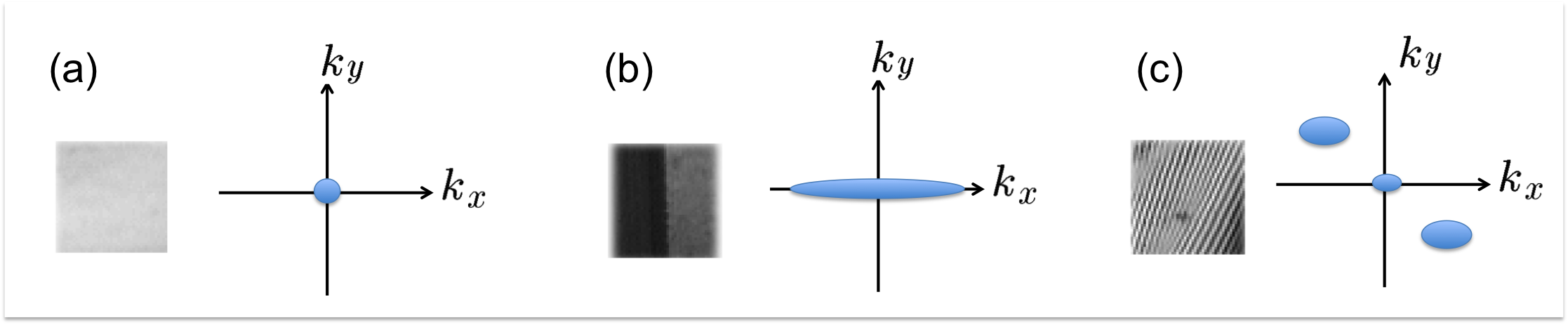
To make this paper self-contained, here we briefly review the origin of the low-rank Hankel matrix as extensively studied in [62, 63].
Note that many types of image patches have sparsely distributed Fourier spectra. For example, as shown in Figure 14(a), a smoothly varying patch usually has spectrum content in the low-frequency regions. For the case of an edge as shown in Figure 14(b), the spectral components are mostly localized along the -axis. Similar spectral domain sparsity can be observed in the texture patch shown in Figure 14(c), where the spectral components of the patch are distributed at the harmonics of the texture. In these cases, if we construct a Hankel matrix using the corresponding image patch, the resulting Hankel matrix is low-ranked [63].
In order to understand this intriguing relationship, consider a 1-D signal, whose spectrum in the Fourier domain is sparse and can be modeled as the sum of Dirac masses:
| (21) |
where refers to the corresponding sequence of the harmonic components in the Fourier domain. Then, the corresponding discrete time-domain signal is given by:
| (22) |
Suppose that we have a -length filter that has the -transform representation [53]
| (23) |
Then, it is easy to see that [53]
| (24) |
Thus, the filter annihilates the signal and is accordingly referred to as the annihilating filter. Moreover, since Eq. (24) can be represented as
the Hankel matrix is rank-deficient. In fact, the rank of the Hankel matrix can be explicitly determined by the size of the minimum-size annihilating filter [63]. Therefore, if the matrix pencil size is chosen bigger than the minimum annihilating filter size, the Hankel matrix is low-ranked.
References
- [1] J. Adler and O. Öktem, Learned primal-dual reconstruction, IEEE Transactions on Medical Imaging (in press), (2018).
- [2] R. Albanese and P. B. Monk, The inverse source problem for Maxwell’s equations, Inverse Problems, 22 (2006), pp. 1023–1035, https://doi.org/10.1088/0266-5611/22/3/018.
- [3] H. Ammari, E. Bretin, J. Garnier, H. Kang, H. Lee, and A. Wahab, Mathematical Methods in Elasticity Imaging, Princeton University Press, New Jersey, USA, 2015.
- [4] H. Ammari, E. Bretin, J. Garnier, and A. Wahab, Time reversal in attenuating acoustic media, vol. 548 of Contemporary Mathematics, American Mathematical Society, Providence, USA, 2011, pp. 151–163.
- [5] H. Ammari, E. Bretin, J. Garnier, and A. Wahab, Time-reversal algorithms in viscoelastic media, European Journal of Applied Mathematics, 24 (2013), pp. 565–600, https://doi.org/10.1017/S0956792513000107.
- [6] H. Ammari, E. Bretin, V. Jugnon, and A. Wahab, Photoacoustic Imaging for Attenuating Acoustic Media, vol. 2035 of Lecture Notes in Mathematics, Springer Verlag, Berlin, 2012, pp. 57–84, https://doi.org/10.1007/978-3-642-22990-9_3.
- [7] H. Ammari, J. Garnier, W. Jing, H. Kang, M. Lim, K. Sølna, and H. Wang, Mathematical and Statistical Methods for Multistatic Imaging, vol. 2098 of Lecture Notes in Mathematics, Springer-Verlag, Chem, 2013.
- [8] B. E. Anderson, M. Griffa, T. J. Ulrich, and P. A. Johnson, Time reversal reconstruction of finite sized sources in elastic media, The Journal of the Acoustical Society of America, 130 (2011), pp. EL219 – EL225, https://doi.org/10.1121/1.3635378.
- [9] S. Antholzer, M. Haltmeier, and J. Schwab, Deep learning for photoacoustic tomography from sparse data, apr 2017, https://arxiv.org/abs/1704.04587. [Version v2, 18 Aug. 2017].
- [10] A. Archer and K. G. Sabra, Two dimensional spatial coherence of the natural vibrations of the biceps brachii muscle generated during voluntary contractions, in IEEE Engineering in Medicine & Biology Society (EMBC’10), Buenos Aires, Argentina, Piscataway, 2010, IEEE, pp. 170–173, https://doi.org/10.1109/IEMBS.2010.5627271.
- [11] W. Bae, J. Yoo, and J. C. Ye, Beyond Deep Residual Learning for Image Restoration: Persistent Homology-Guided Manifold Simplification, in Computer Vision and Pattern Recognition Workshops (CVPRW), 2017 IEEE Conference on, IEEE, 2017, pp. 1141–1149, https://doi.org/10.1109/CVPRW.2017.152.
- [12] A. Beck and M. Teboulle, Fast gradient-based algorithms for constrained total variation image denoising and deblurring problems, IEEE Transactions on Image Processing, 18 (2009), pp. 2419–2434, https://doi.org/10.1109/TIP.2009.2028250.
- [13] C. Canuto, M. Y. Hussaini, A. Quarteroni, and T. A. Zang, Spectral methods in fluid dynamics, Springer Series in Computational Physics, Springer, Berlin, Heidelberg, 1988, https://doi.org/10.1007/978-3-642-84108-8.
- [14] H. Chen, Y. Zhang, Y. Chen, J. Zhang, W. Zhang, H. Sun, Y. Lv, P. Liao, J. Zhou, and G. Wang, LEARN: Learned experts? assessment-based reconstruction network for sparse-data CT, IEEE Transactions on Medical Imaging (in press), (2018).
- [15] H. Chen, Y. Zhang, M. K. Kalra, F. Lin, Y. Chen, P. Liao, J. Zhou, and G. Wang, Low-dose CT with a residual encoder-decoder convolutional neural network, IEEE transactions on medical imaging, 36 (2017), pp. 2524–2535, https://doi.org/10.1109/TMI.2017.2715284.
- [16] H. Chen, Y. Zhang, W. Zhang, P. Liao, K. Li, J. Zhou, and G. Wang, Low-dose CT via convolutional neural network, Biomedical Optics Express, 8 (2017), pp. 679–694, https://doi.org/10.1364/BOE.8.000679.
- [17] D. L. Donoho, Compressed sensing, IEEE Transactions on Information Theory, 52 (2006), pp. 1289–1306, https://doi.org/10.1109/TIT.2006.871582.
- [18] F. C. et al., Keras, 2015.
- [19] M. Fink, D. Cassereau, A. Derode, C. Prada, P. Roux, M. Tanter, J.-L. Thomas, and F. Wu, Time-reversed acoustics, Reports on Progress in Physics, 63 (2000), pp. 1933–1994, https://doi.org/10.1088/0034-4885/63/12/202.
- [20] J.-L. Gennisson, S. Catheline, S. Chaffaı̈, and M. Fink, Transient elastography in anisotropic medium: Application to the measurement of slow and fast shear wave speeds in muscles, The Journal of the Acoustical Society of America, 114 (2003), pp. 536 – 541, https://doi.org/10.1121/1.1579008.
- [21] M. Griffa, B. E. Anderson, R. A. Guyer, T. J. Ulrich, and P. A. Johnson, Investigation of the robustness of time reversal acoustics in solid media through the reconstruction of temporally symmetric sources, Journal of Physics D: Applied Physics, 41 (2008), p. 085415, https://doi.org/10.1088/0022-3727/41/8/085415.
- [22] Y. Han and J. C. Ye, Framing U-Net via Deep Convolutional Framelets: Application to Sparse-view CT, IEEE Transactions on Medical Imaging (in press), (2018).
- [23] Y. Han, J. Yoo, and J. C. Ye, Deep residual learning for compressed sensing CT reconstruction via persistent homology analysis, nov 2016, https://arxiv.org/abs/1611.06391. [Version v2, 25 Nov. 2016].
- [24] F. D. Hastings, J. B. Schneider, and S. L. Broschat, Application of the perfectly matched layer (PML) absorbing boundary condition to elastic wave propagation, The Journal of the Acoustical Society of America, 100 (1996), pp. 3061–3069, https://doi.org/10.1121/1.417118.
- [25] K. H. Jin, D. Lee, and J. C. Ye, A general framework for compressed sensing and parallel MRI using annihilating filter based low-rank Hankel matrix, IEEE Transactions on Computational Imaging, 2 (2016), pp. 480–495, https://doi.org/10.1109/TCI.2016.2601296.
- [26] K. H. Jin, M. T. McCann, E. Froustey, and M. Unser, Deep convolutional neural network for inverse problems in imaging, IEEE Transactions on Image Processing, 26 (2017), pp. 4509 – 4522, https://doi.org/10.1109/TIP.2017.2713099.
- [27] K. H. Jin and J. C. Ye, Annihilating filter-based low-rank Hankel matrix approach for image inpainting, IEEE Transactions on Image Processing, 24 (2015), pp. 3498–3511, https://doi.org/10.1109/TIP.2015.2446943.
- [28] E. Kang, W. Chang, J. Yoo, and J. C. Ye, Deep convolutional framelet denosing for low-dose CT via wavelet residual network, IEEE Transactions on Medical Imaging (in press), (2018).
- [29] E. Kang, J. Min, and J. C. Ye, A deep convolutional neural network using directional wavelets for low-dose X-ray CT reconstruction, Medical Physics, 44 (2017), pp. e360–e375, https://doi.org/10.1002/mp.12344.
- [30] E. Kang and J. C. Ye, Wavelet domain residual network (WavResNet) for low-dose X-ray CT reconstruction, 2017, https://arxiv.org/abs/1703.01383.
- [31] A. Karpathy and L. Fei-Fei, Deep visual-semantic alignments for generating image descriptions, IEEE Transactions on Pattern Analysis and Machine Intelligence, 39 (2017), pp. 664–676.
- [32] S. Kedar, Source distribution of ocean microseisms and implications for time-dependent noise tomography, Comptes Rendus Geoscience, 343 (2011), pp. 548 – 557, https://doi.org/10.1016/j.crte.2011.04.005.
- [33] D. P. Kingma and J. Ba, Adam: A method for stochastic optimization, 2014, https://arxiv.org/abs/1412.6980. [Version v9, 30 Jan. 2017].
- [34] S. Kremers, A. Fichtner, G. B. Brietzke, H. Igel, C. Larmat, L. Huang, and M. Käser, Exploring the potentials and limitations of the time-reversal imaging of finite seismic sources, Solid Earth, 2 (2011), pp. 95–105, https://doi.org/10.5194/se-2-95-2011.
- [35] A. Krizhevsky, I. Sutskever, and G. E. Hinton, Imagenet classification with deep convolutional neural networks, in Proceedings of the 25th International Conference on Neural Information Processing Systems - Volume 1, USA, 2012, Curran Associates Inc., pp. 1097–1105.
- [36] A. Lakhal and A. K. Louis, Locating radiating sources for Maxwell’s equations using the approximate inverse, Inverse Problems, 24 (2008), p. 045020, https://doi.org/10.1088/0266-5611/24/4/045020.
- [37] C. Larmat, J.-P. Montagner, M. Fink, Y. Capdeville, A. Tourin, and E. Clévédé, Time-reversal imaging of seismic sources and application to the great sumatra earthquake, Geophysical Research Letters, 33 (2006), https://doi.org/10.1029/2006GL026336.
- [38] D. D. Lee and H. S. Seung, Unsupervised learning by convex and conic coding, in Advances in Neural Information Processing Systems, MIT Press, 1997, pp. 515–521, https://doi.org/10.1.1.55.6629.
- [39] D. D. Lee and H. S. Seung, Learning the parts of objects by non-negative matrix factorization, Nature, 401 (1999), p. 788, https://doi.org/10.1038/44565.
- [40] D. D. Lee and H. S. Seung, Algorithms for non-negative matrix factorization, in Proceedings of the 13th International Conference on Neural Information Processing Systems, Cambridge, MA, USA, 2000, MIT Press, pp. 535–541.
- [41] J. Lim, A. Wahab, G. Park, K. Lee, Y. Park, and J. C. Ye, Beyond born-rytov limit for super-resolution optical diffraction tomography, Optics Express, 25 (2017), pp. 30445–30458, https://doi.org/10.1364/OE.25.030445.
- [42] Y. Liu, T. Zhao, W. Ju, and S. Shi, Materials discovery and design using machine learning, Journal of Materiomics, 3 (2017), pp. 159–177, https://doi.org/10.1016/j.jmat.2017.08.002.
- [43] Y. Liu, T. Zhao, G. Yang, W. Ju, and S. Shi, The onset temperature (Tg) of AsxSe 1- x glasses transition prediction: A comparison of topological and regression analysis methods, Computational Materials Science, 140 (2017), pp. 315–321, https://doi.org/10.1016/j.commatsci.2017.09.008.
- [44] C. H. McCollough, A. C. Bartley, R. E. Carter, B. Chen, T. A. Drees, P. Edwards, D. R. Holmes, A. E. Huang, F. Khan, S. Leng, et al., Low-dose CT for the detection and classification of metastatic liver lesions: Results of the 2016 low dose CT grand challenge, Medical Physics, 44 (2017), https://doi.org/10.1002/mp.12345.
- [45] C. M. Michel, M. M. Murray, G. Lantz, S. Gonzalez, L. Spinelli, and R. G. de Peralta, EEG source imaging, Clinical Neurophysiology, 115 (2004), pp. 2195 – 2222, https://doi.org/10.1016/j.clinph.2004.06.001.
- [46] V. Nair and G. E. Hinton, Rectified linear units improve restricted Boltzmann machines, in Proceedings of the 27th international conference on machine learning (ICML-10), 2010, pp. 807–814.
- [47] R. P. Porter and A. J. Devaney, Holography and the inverse source problem, Journal of the Optical Society of America, 72 (1982), pp. 327 – 330, https://doi.org/10.1364/JOSA.72.000327.
- [48] O. Ronneberger, P. Fischer, and T. Brox, U-net: Convolutional networks for biomedical image segmentation, in Medical Image Computing and Computer-Assisted Intervention – MICCAI 2015, N. Navab, J. Hornegger, W. Wells, and A. Frangi, eds., vol. 9351 of Lecture Notes in Computer Science, Cham, nov 2015, Springer, pp. 234 – 241, https://doi.org/10.1007/978-3-319-24574-4_28.
- [49] O. Russakovsky, J. Deng, H. Su, J. Krause, S. Satheesh, S. Ma, Z. Huang, A. Karpathy, A. Khosla, M. Bernstein, A. C. Berg, and L. Fei-Fei, ImageNet Large Scale Visual Recognition Challenge, International Journal of Computer Vision (IJCV), 115 (2015), pp. 211–252, https://doi.org/10.1007/s11263-015-0816-y.
- [50] K. G. Sabra, S. Conti, P. Roux, and W. A. Kuperman, Passive in vivo elastography from skeletal muscle noise, Applied Physics Letters, 90 (2007), p. 194101, https://doi.org/10.1063/1.2737358.
- [51] O. Scherzer(ed.), Handbook of Mathematical Methods in Imaging, Springer, New York, 1st ed., 2011.
- [52] S. Shi, J. Gao, Y. Liu, Y. Zhao, Q. Wu, W. Ju, C. Ouyang, and R. Xiao, Multi-scale computation methods: Their applications in lithium-ion battery research and development, Chinese Physics B, 25 (2015), p. 018212, https://doi.org/10.1088/1674-1056/25/1/018212.
- [53] M. Vetterli, P. Marziliano, and T. Blu, Sampling signals with finite rate of innovation, IEEE Transactions on Signal Processing, 50 (2002), pp. 1417–1428, https://doi.org/10.1109/TSP.2002.1003065.
- [54] A. Wahab and R. Nawaz, A note on elastic noise source localization, Journal of Vibration and Control, 22 (2016), pp. 1889 –1894, https://doi.org/10.1177/1077546314546511.
- [55] A. Wahab, A. Rasheed, T. Hayat, and R. Nawaz, Electromagnetic time reversal algorithms and source localization in lossy dielectric media, Communications in Theoretical Physics, 62 (2014), pp. 779–789, https://doi.org/10.1088/0253-6102/62/6/02.
- [56] G. Wang, A perspective on deep imaging, IEEE Access, 4 (2016), pp. 8914–8924, https://doi.org/10.1109/ACCESS.2016.2624938.
- [57] S. Wang, Z. Su, L. Ying, X. Peng, S. Zhu, F. Liang, D. Feng, and D. Liang, Accelerating magnetic resonance imaging via deep learning, in Biomedical Imaging (ISBI), 2016 IEEE 13th International Symposium on, IEEE, 2016, pp. 514–517, https://doi.org/10.1109/ISBI.2016.7493320.
- [58] X. Wang, M. Song, Y. Guo, H. Li, and H. Liu, Fourier method for identifying electromagnetic sources with multi-frequency far-field data, jan 2018, https://arxiv.org/abs/1801.03263.
- [59] A. Wiegmann, Fast poisson, fast Helmholtz and fast linear elastostatic solvers on rectangular parallelepipeds, tech. report, Ernest Orlando Lawrence Berkeley National Laboratory, Berkeley, CA (US), 1999.
- [60] J. M. Wolterink, T. Leiner, M. A. Viergever, and I. Išgum, Generative adversarial networks for noise reduction in low-dose CT, IEEE Transactions on Medical Imaging, 36 (2017), pp. 2536–2545, https://doi.org/10.1109/TMI.2017.2708987.
- [61] T. Würfl, F. C. Ghesu, V. Christlein, and A. Maier, Deep learning computed tomography, in International Conference on Medical Image Computing and Computer-Assisted Intervention, Springer, 2016, pp. 432–440, https://doi.org/10.1007/978-3-319-46726-9_50.
- [62] J. C. Ye, Y. Han, and E. Cha, Deep convolutional framelets: A general deep learning framework for inverse problems, SIAM Journal on Imaging Sciences, 11 (2018), pp. 991–1048, https://doi.org/10.1137/17M1141771.
- [63] J. C. Ye, J. M. Kim, K. H. Jin, and K. Lee, Compressive sampling using annihilating filter-based low-rank interpolation, IEEE Transactions on Information Theory, 63 (2017), pp. 777 – 801, https://doi.org/10.1109/TIT.2016.2629078.
- [64] J. Yoo, Y. Jung, M. Lim, J. C. Ye, and A. Wahab, A joint sparse recovery framework for accurate reconstruction of inclusions in elastic media, SIAM Journal on Imaging Sciences, 10 (2017), pp. 1104–1138, https://doi.org/10.1137/16M110318X.
- [65] D. Zhang, Y. Guo, J. Li, and H. Liu, Locating multiple multipolar acoustic sources using the direct sampling method, jan 2018, https://arxiv.org/abs/1801.05584.
- [66] K. Zhang, W. Zuo, Y. Chen, D. Meng, and L. Zhang, Beyond a gaussian denoiser: Residual learning of deep CNN for image denoising, IEEE Transactions on Image Processing, 26 (2017), pp. 3142 – 3155, https://doi.org/10.1109/TIP.2017.2662206.