On optimal designs for non-regular models

To start, we consider the scalar case with $d=1$. Suppose that there exists a constant $\alpha\in(0,2]$ such that, for each $\theta$, the limit $J(\theta)=\lim_{\varepsilon\to 0}|\varepsilon|^{-\alpha}h(\theta;\theta+\varepsilon)$ exists, is finite, and non-zero. If such an $\alpha$ exists, then it must be unique; but there are cases where existence fails, e.g., when $\theta$ is not identifiable, so that $h(\theta,\theta+\varepsilon)\equiv 0$ for all sufficiently small $\varepsilon$. The case $\alpha=2$ corresponds to differentiable in quadratic mean and, hence, “regular,” while $\alpha\in(0,2)$ corresponds to “non-regular.” Differentiability of $\vartheta\mapsto H(P_{\theta},P_{\vartheta})$ or lack thereof determines a model’s regularity, so the largest value $\alpha$ can take is 2; otherwise, the limit is infinite. From the above limit, there is a local approximation,

This resembles the local Hölder condition considered in Ibragimov and Hasminskii, (1981, Section I.6). We call $\alpha$ the index of regularity and $J(\theta)$ the Hellinger information. Of course, if $\alpha=2$, then $J(\theta)$ is proportional to $I(\theta)$, the Fisher information. Next are a few quick examples, all with $\alpha=1$.

• •

  If $P_{\theta}={\sf Unif}(0,\theta)$, $\theta>0$, then $J(\theta)=\theta^{-1}$.

• •

  If $P_{\theta}={\sf Unif}(\theta^{-1},\theta)$, $\theta>1$, then $J(\theta)=(\theta^{2}+1)\{\theta(\theta^{2}-1)\}^{-1}$.

• •

  If $P_{\theta}={\sf Unif}(\theta;\theta^{2})$, $\theta>1$, then $J(\theta)=(2\theta+1)\{\theta(\theta-1)\}^{-1}$.

A class of non-regular models of particular interest to us here are those in Smith, (1994) based on location shifts of distributions supported on the positive half-line. Consider a density $p_{0}$ on $(0,\infty)$ that satisfies

where $\beta\geq 1$ and $c=c(\beta)\in(0,\infty)$. For example, the gamma and Weibull families, with shape parameter $\beta$ and scale $\sigma$, have $c=\{\beta\sigma^{\beta}\Gamma(\beta)\}^{-1}$ and $c=\sigma^{-\beta}$, respectively. The next result identifies the regularity index $\alpha$ and the Hellinger information $J(\theta)$ for this class of location parameter problems, with $p_{\theta}(y)=p_{0}(y-\theta)$. It shows that $\alpha$ need not be an integer and the Hellinger information, like Fisher’s, is constant in location models. When $\beta\geq 2$, the model is regular—with $\alpha=2$ and the Fisher information defined as usual—so we focus here on the non-regular case with $\beta\in[1,2)$.

Ibragimov and Hasminskii, (1981, Theorem VI.1.1) show that, in this case, $h(\theta;\theta+\varepsilon)=O(|\varepsilon|^{\beta})$ as $\varepsilon\to 0$, but they do not identify $J(\theta)$. Similar results have appeared elsewhere in the literature on non-regular models; our condition (4) is basically the same as Condition $C_{5}$ in Woodroofe, (1974), which is basically the same as Assumption 9 in Smith, (1985).

Turning to the general, non-regular multi-parameter case, where $\Theta$ is an open subset of $\mathbb{R}^{d}$, defining Hellinger information requires some additional effort. In particular, non-regularity implies that the familiar local quadratic approximation of $h$ fails, so we should not expect to have an “information matrix” to describe the local behavior in such cases. In fact, $h(\theta;\vartheta)$ depends locally on the direction along which $\vartheta$ approaches $\theta$, so there is no “direction-free” summary of the local structure and, hence, no “information matrix”; see Remark 2. But this lack of a convenient quadratic approximation need not stop us from defining a suitable Hellinger information.

Since the approximation (7) is in terms of $|\varepsilon|$, it follows that $J(\theta;u)=J(\theta;-u)$, so $J(\theta;u)$ really only depends on the line defined by $u$. If $d=1$, then there is only one line, i.e., $u=\pm 1$, hence, for the scalar case, we can drop the $u$ argument entirely and write $J(\theta)$ as described above. It is also worth pointing out that Definition 1 assumes that a single index $\alpha$ suffices to describe the regularity of a model with a $d$-dimensional parameter. This is appropriate for the kinds of regression models we have in mind here, but can be a limitation in other cases; see Remark 1 below.

As a quick example, let $P_{\theta}={\sf Unif}(\theta_{1},\theta_{1}+\theta_{2})$, where $\theta_{1}\in\mathbb{R}$ and $\theta_{2}>0$. In this form, $\theta_{1}$ and $\theta_{2}$ are location and scale parameters, respectively. If $u=(u_{1},u_{2})$ is a generic vector on the unit circle, then $J(\theta;u)=\theta_{2}^{-1}g(u)$, where $g(u)$ has a form which is slightly too complicated to present here; see Section S1 in the Supplementary Material. This expression agrees with the familiar properties of Fisher information for location–scale models.

Although we do not define an “information matrix” in the non-regular case (see Remark 2), when the model is regular, i.e., when $\alpha=2$, there are still some connections between our Hellinger information and the familiar Fisher information. In particular, $J(\theta;u)$ is a quadratic form involving the Fisher information $I(\theta)$ and the direction $u$. This gives an alternative explanation of how the regular models admit a separation of the dependence on $\theta$ and on the direction $u$ of departure from $\theta$.

Another useful and familiar feature of Fisher information that also holds for Hellinger information is the reparametrization formula (Proposition 3), which comes in handy for regression problems where the natural parameter is expressed as a function of covariates and another parameter.

We now return to our original setup where $Y_{1},\ldots,Y_{n}$ are independent, but not necessarily identically distributed, with $Y_{i}\sim P_{i,\theta}$, $i=1,\ldots,n$, and $\theta$ is an unknown parameter taking values in an open subset $\Theta$ of $\mathbb{R}^{d}$ for some $d\geq 1$. Let $P_{\theta}^{n}$ denote the joint distribution of $Y^{n}=(Y_{1},\ldots,Y_{n})$. Motivated by the regression problems below, we assume that each $P_{i,\theta}$ has the same index of regularity, $\alpha\in(0,2]$. Following our intuition from the regular case, define the Hellinger information at $\theta$, in the direction of $u$, based on the sample of size $n$, as

where $J_{i}(\theta;u)$ is the Hellinger information based on $P_{i,\theta}$ as described above. See Remark 3 for more on this additivity property. Theorem 1 below will establish a suitable connection between $\mathcal{J}_{n}(\theta;u)$ and the quality of an estimator, and this will provide the necessary foundation for defining optimal designs for non-regular models.

Suppose the goal is to estimate $\psi(\theta)$, where $\psi:\mathbb{R}^{d}\to\mathbb{R}^{q}$, $q\leq d$, is sufficiently smooth. Let $T_{n}=T(Y^{n})$ be an estimator of $\psi(\theta)$, and measure its quality by the risk

the $q$-vector version of mean square error, where expectation, $E_{\theta}^{n}$, is with respect to $P_{\theta}^{n}$. This covers the case where $\psi(\theta)=\theta$ and $q=d$, so that interest is in the full parameter $\theta$, and the case where $\psi(\theta)$ is a single component of $\theta$ and $q=1$, as well as other intermediate cases. Next is the aforementioned lower bound on the risk in terms of the total Hellinger information.

Two very brief comments: first, the universal constant hidden in “$\gtrsim$” is known and given in the proof; second, there is nothing special about “3” in the definition of $\varepsilon_{n,u}$, any number strictly greater than 2 would suffice.

Some additional comments about the interpretation of Theorem 1 are in order. First, the reason for taking supremum over a small “neighborhood” of $\theta$ is that a lucky choice of $T_{n}\equiv\psi(\theta)$ has excellent performance at $\theta$, but poor performance at a nearby $\vartheta$. The theorem basically says that, if one looks at a locally uniform measure of risk, which prevents “cheating” towards or luck at a particular $\theta$, then one cannot have smaller risk than that in the lower bound (11). The classical Cramér–Rao lower bound uses unbiasedness of the estimator to prevent this kind of cheating/luck.

To assess the sharpness of the bound in (11) when regularity conditions do not apply, consider the case where $q=1$, so that $\psi(\theta)$ is a scalar function. For the rate, if we consider the identically independently distributed case, so that $\mathcal{J}_{n}(\theta;u)=nJ_{1}(\theta;u)$, then it follows that the lower bound is of order $n^{-2/\alpha}$, which agrees with the known minimax rate for estimators in non-regular models (Ibragimov and Hasminskii, 1981, Sec. I.5). Therefore, the bound cannot be improved in terms of dependence on the sample size. To assess the quality of the lower bound in terms of its dependence on $\theta$, if the observations come from ${\sf Unif}(0,\theta)$, which has $\alpha=1$ and $J(\theta)=\theta^{-1}$, the maximum likelihood estimator is the sample maximum, and its mean square error is given by

Asymptotically, this expression is proportional to $\theta^{2}n^{-2}$, which agrees with our lower bound. Therefore, up to universal constants, the bound in Theorem 1 is sharp. Whether there exists an estimator that can attain the bound exactly or asymptotically is unclear in general; see Remark 4.

It is worth stating the special case where $\alpha=2$ as a corollary to Theorem 1. This reveals some connection to the classical Cramér–Rao bound, even though we do not have access to an information matrix, and demonstrates the generality of our result.

For comparison to the classical setting, if we take $\psi(\theta)=\theta$, then the expression in the above display simplifies to

Wanting the information matrix to have a large minimal eigenvalue is a familiar concept in the classical optimal design theory; see Section 4.

This and the previous subsection, along with the remarks in Section 3.3, establish some important properties and insights concerning our proposed Hellinger information. A difficulty that has not yet been addressed is the dependence of $\mathcal{J}_{n}(\theta;u)$ on the arbitrary direction $u$. However, the lower bound in (11) is free of a direction, so it makes sense to formulate a direction-free Hellinger information based on that. For a non-regular model as formulated above, with index of regularity $\alpha\in(0,2]$, we set the direction-free Hellinger information at $\theta$, for interest parameter $\psi(\theta)$, as

In the special case where $\psi(\theta)=\theta$, this simplifies to

Moreover, in the regular case with $\alpha=2$, it follows from Corollary 1 and, in particular, (12), that $\mathcal{J}_{n}(\theta)$ above is (proportional to) the smallest eigenvalue of the Fisher information matrix. Therefore, definition (13) seems very reasonable; more details are presented in Section 4.

The previous section built up a framework of information, based on a local approximation of the squared Hellinger distance, suitable for non-regular problems where Fisher information does not exist. Our motivation for building such a framework was to address the problem of optimal experimental designs in cases where the underlying statistical model is non-regular. This section defines what we mean by an optimal design for non-regular models, and provides some additional details about the Hellinger information that are particularly relevant to the design problem.

We start here with a slightly different setup than in the previous section, but quickly connect it back to the preceding. Let $Y_{1},\ldots,Y_{n}$ be independent observations, where $Y_{i}$ has density function $q_{\eta_{i}}$, for $i=1,\ldots,n$. That is, each $Y_{i}$ has its own parameter $\eta_{i}$, which we will assume is real-valued, as is typical in linear and generalized linear models. Then the design problem proceeds by expressing the unit-specific parameter $\eta_{i}$ as a given function $g(x_{i},\theta)$ of a common parameter $\theta\in\mathbb{R}^{d}$ and a vector of unit-specific covariates; here, of course, the covariates are constants that the investigator is able to set in any way he/she pleases, but preferably in a way that is “optimal” in some sense. By linking each $\eta_{i}$ to a common $\theta$, we obtain the setup from previous sections, i.e., $Y_{i}\sim p_{i,\theta}$, independent, for $i=1,\ldots,n$.

The next result, stated in the context of $n=1$, parallels a familiar one in the regular case for Fisher information. It aids in computing the Hellinger information under a reparametrization like the one described above.

From the general theory in Section 3, if $Y_{1},\ldots,Y_{n}$ are independent, then under the assumptions in Proposition 3, i.e., $Y_{i}\sim p_{i,\theta}=q_{g_{i}(\theta)}$, the Hellinger information at $\theta$, in direction of $u$, is

For the special case where $g_{i}(\theta)=g(x_{i},\theta)$ for covariates $x_{i}$, it is clear that $\mathcal{J}_{n}(\theta;u)$ depends on $x_{1},\ldots,x_{n}$. For example, if $Y_{1},\ldots,Y_{n}$ are independent, with $Y_{i}\sim g(x_{i},\theta)+{\sf Gamma}(\beta,1)$, where $g(x,\theta)=\theta_{0}+\sum_{k=1}^{p}\theta_{k}x^{k+1}$, then it follows from Propositions 1 and 3 that

The Hellinger information’s dependence on the covariates $(x_{1},\ldots,x_{n})$ is what makes our theory of optimal design possible.

In what follows, we focus exclusively on the case of $\psi(\theta)=\theta$, and the direction-free definition of Hellinger distance in (14), though this is only for simplicity. The same derivations can be carried out with any specific interest parameter $\psi(\theta)$ in mind.

Following the now-standard approximate design theory put forth by Kiefer, (1974), let $\xi$ denote a discrete probability measure defined on the design space—the space where the covariates $x_{i}$ live—with at most $m$ distinct atoms, representing the design itself. That is, the atoms of $\xi$ represent the specific design points, and the probabilities correspond to the weights (more details below). Next, with a slight abuse of our previous notation, we write $\mathcal{J}_{\xi}(\theta;u)$ to indicate that the Hellinger information in the direction $u$ depends on the design $\xi$ through the specific covariate values. For example, given design $\xi=\{(w_{i},x_{i}):i=1,...,m\}$, then $\mathcal{J}_{\xi}(\theta;u)=\sum_{i=1}^{m}w_{i}J_{i}(\theta;u)$, where $J_{i}(\theta;u)$ is the Hellinger information in the direction $u$ based on one observation taken at location $x_{i}$. Following (14), the Hellinger information based on design $\xi$ is defined as

Naturally, the optimal design under this setup would be defined as the one that maximizes this measure of information.

For comparison to the classical design theory, property (12) implies that our optimal design in Definition 2, under a regular model, corresponds to an E-optimal design, one that maximizes the minimum eigenvalue of the Fisher information matrix. For the non-regular case, however, we do not have an information matrix, so it is not clear if other common notions of optimality, such as A- and D-optimality, have any meaning. For example, non-regularity will cause sampling distributions of estimators to be non-ellipsoidal, so we cannot expect the determinant of some information matrix to correspond to the volume of a confidence ellipsoid.

Definition 2 formulates a new class of optimal design problems, deserving further attention. As discussed briefly in Section 1, there is now a substantial literature on theory and computation related to the optimal design problem in regular cases, and we hope that this paper stimulates a parallel line of work with similar developments for non-regular cases. There are some similarities to the regular case, in particular, the Hellinger information is non-negative and additive like Fisher information. Also, the map $\xi\mapsto\mathcal{J}_{\xi}(\theta)$ is concave for fixed $\theta$, i.e., for any two designs $\xi$ and $\xi^{\prime}$ and any $w\in[0,1]$,

which is important for numerical and/or analytical solution of the optimal design problem. The following gives some first results along these lines.

Motivated by the setup in Smith, (1994), we consider a non-regular model of the form

where $x_{i}$ are scalars, $g(x,\theta)=\theta_{0}+\sum_{k=1}^{p}\theta_{k}x^{k}$ is a degree-$p$ polynomial, $\theta\in\mathbb{R}^{d}$, with $d=p+1$, is an unknown parameter, and $\varepsilon_{i}$ are independent and identically distributed with density $p_{0}$ given in (3) and known shape parameter $\alpha\in[1,2)$. As is customary (Koenker and Hallock, 2001, e.g.,), we will insist that the design points be centered at the origin, which puts a constraint on the design itself. In particular, we will consider the space of designs $\xi$ given by

i.e., designs on $[-A,A]$ that are “balanced” in the sense that the mean $x$ value is 0, where $A>0$ is fixed and known.

The following result shows that, among balanced designs, the subclass of symmetric designs is complete in the sense that the maximum information over symmetric designs is the same as that over the larger class of balanced designs. This implies that the search for an optimal design can be simplified by restricting it to the smaller class of symmetric designs.

The next section applies this general result to identify optimal designs in some special cases of the non-regular polynomial regression model above. The two results, Propositions 4 and 5, suggest that there is a de la Garza phenomenon (de la Garza, 1954, e.g.,) in the non-regular case as well, which would be an interesting theoretical topic to pursue in future work.

Consider the linear version of (16), where $g(x,\theta)=\theta_{0}+\theta_{1}x$. For linear models we have a strong intuition from the regular case as to what the optimal design might be. It turns out that the same result holds in the non-regular case as well.

Consider a quadratic case where $g(x,\theta)=\theta_{0}+\theta_{1}x+\theta_{2}x^{2}$. Here we restrict our attention to the case where the errors $\varepsilon_{i}$ in the model are exponential, $\alpha=1$.

Although the proof of Proposition 5 holds only for the $\alpha=1$ case, we expect that the result also holds for $\alpha\in[1,2)$, and the numerical results in Figure 3 (b) support this conjecture. The practical importance is that it simplifies the search over $\Xi_{\mathrm{sym}}$ to a search over the scalar $\pi\in[0,1]$. The weight at point $\{0\}$ of the optimal design—or the likely optimal design for the case of $\alpha\in(1,2]$—depends on the value of $A$ and $\alpha$. Based on Proposition 5 and the definition of Hellinger information, the optimal weight can be obtained by solving the optimization problem

where $f(\pi)=f_{\alpha,A}(\pi)$ is given by

This search for the optimal weight, $\pi_{A}(\alpha)$, along with that over $u$ on the surface of the unit sphere, can be handled numerically.

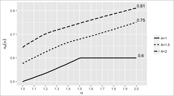
Figure 1 shows $\alpha\mapsto\pi_{A}(\alpha)$ for several values of $A$. In particular, we see that the (likely) optimal designs put more weight on 0 as either $\alpha$ or $A$ increases. Our optimal designs for non-regular regression models have a similar format to their E-optimal counterparts in the regular case. That is, a regular E-optimal design for quadratic regression over $[-A,A]$ is given by

and, for $A$ in $\{1,1.5,2\}$, the corresponding values of $w_{A}$ are $\{0.6,0.75,0.81\}$. From Figure 1, as anticipated by Corollary 1, we observe that for $\alpha=2$, $\pi_{A}(2)$ matches the weight $w_{A}$ of the corresponding regular E-optimal design. This is explained by Corollary 1; when $\alpha=2$, optimal design under Hellinger information is the E-optimal design.

Henceforth, we call the regular E-optimal design counterpart of a non-regular model “regular-optimal.” For the non-regular linear model, based on Proposition 4, the optimal design coincides with the “regular-optimal” design. In the numerical results presented below, we compare optimal designs of non-regular quadratic models to their “regular-optimal” counterparts.

Here we show some numerical results to demonstrate the efficiency gain in using the proposed optimal designs over other reasonable designs. Recall our model is of the form (16) with non-negative errors having density (3), with known shape parameter $\alpha\in[1,2)$.

One complication is that currently there are no results that identify an estimator whose risk attains the lower bound in Theorem 1. Consequently, we are currently unable to guarantee that minimizing this lower bound will result in improved estimation for any given estimator. But we do have a reasonable estimator, described next, and the results below do indicate that the design that minimizes the lower bound in Theorem 1 does indeed result in improved efficiency for this particular estimation.

For the class of non-regular polynomial regression problems in consideration here, Smith, (1994) proposed an estimator based on solving a linear programming problem: choosing $(\theta_{0},\ldots,\theta_{p})$ such that $\theta_{0}$ is maximized subject to the condition that $y_{i}\geq\sum_{k=1}^{p}\theta_{k}x_{i}^{k}$ for each $i=1,\ldots,n$. This estimator agrees with the maximum likelihood estimator in the case $\alpha=1$, has a $O(n^{-1/\alpha})$ convergence rate, which matches the one given by the lower bound in (11), and can be readily computed using the quantreg package in R (Koenker, 2013). Moreover, as Smith, (1994, p. 174) argues, it is generally superior to maximum likelihood in non-regular cases. For these reasons, comparisons of designs based on this estimator ought to be informative.

Figure 2 presents simulation results on the quality of estimation for the Hellinger optimal design versus 5-, 10-, and 15-point uniform designs for the non-regular linear models, while Figure 3 presents simulation results comparing Hellinger optimal design versus 5-point uniform design and the regular-optimal design. The study proceeds as follows. For each design space $[-A,A]$ and candidate design, the $n$-vector $y$ is simulated from the corresponding model, with the specified value of $\alpha$ and $\theta$, and then Smith’s estimator $\hat{\theta}$ is computed. Repeat this process 1000 times and compute the Monte Carlo estimate of the risk $R(\hat{\theta},\theta)$ as usual. This risk is the sum of mean square errors for each component of the parameter vector.

Figure 2 shows that, under different regularity conditions, the optimal design from Proposition 4 is superior in terms of risk. In particular, it is significantly better in the estimation of the slope, $\theta_{1}$, whereas no design performs significantly better than the others in the estimation of the intercept. The results presented in Figure 3(a) are consistent with Proposition 5 in the case of $\alpha=1$. In each case, the optimal design performs significantly better than both the 5-point uniform design and the regular-optimal design, despite the similarity of the optimal and regular-optimal designs in terms of weight at point 0. Similarly, Figure 3(b) supports our intuition that Proposition 5 can be extended to cases with $\alpha>1$.

References

- Bernardo, (1979) Bernardo, J.-M. (1979). Reference posterior distributions for Bayesian inference. J. Roy. Statist. Soc. Ser. B, 41(2):113–147. With discussion.
- Biedermann et al., (2009) Biedermann, S., Dette, H., and Hoffmann, P. (2009). Constrained optimal discrimination designs for Fourier regression models. Ann. Inst. Statist. Math., 61(1):143–157.
- Biedermann et al., (2011) Biedermann, S., Dette, H., and Woods, D. C. (2011). Optimal design for additive partially nonlinear models. Biometrika, 98(2):449–458.
- Biedermann et al., (2006) Biedermann, S., Dette, H., and Zhu, W. (2006). Optimal designs for dose-response models with restricted design spaces. J. Amer. Statist. Assoc., 101(474):747–759.
- Chernozhukov and Hong, (2004) Chernozhukov, V. and Hong, H. (2004). Likelihood estimation and inference in a class of nonregular econometric models. Econometrica, 72(5):1445–1480.
- Cousineau, (2009) Cousineau, D. (2009). Fitting the three-parameter Weibull distribution: Review and evaluation of existing and new methods. IEEE Transactions on Dielectrics and Electrical Insulation, 16(1):281–288.
- de la Garza, (1954) de la Garza, A. (1954). Spacing of information in polynomial regression. Ann. Math. Statistics, 25:123–130.
- Dette et al., (2008) Dette, H., Bretz, F., Pepelyshev, A., and Pinheiro, J. (2008). Optimal designs for dose-finding studies. J. Amer. Statist. Assoc., 103(483):1225–1237.
- Dette et al., (2018) Dette, H., Guchenko, R., Melas, V. B., and Wong, W. K. (2018). Optimal discrimination designs for semiparametric models. Biometrika, 105(1):185–197.
- Dette et al., (2017) Dette, H., Konstantinou, M., and Zhigljavsky, A. (2017). A new approach to optimal designs for correlated observations. Ann. Statist., 45(4):1579–1608.
- Dette and Melas, (2011) Dette, H. and Melas, V. B. (2011). A note on the de la Garza phenomenon for locally optimal designs. Ann. Statist., 39(2):1266–1281.
- Dette et al., (2016) Dette, H., Pepelyshev, A., and Zhigljavsky, A. (2016). Optimal designs in regression with correlated errors. Ann. Statist., 44(1):113–152.
- Dette and Schorning, (2013) Dette, H. and Schorning, K. (2013). Complete classes of designs for nonlinear regression models and principal representations of moment spaces. Ann. Statist., 41(3):1260–1267.
- Dette and Titoff, (2009) Dette, H. and Titoff, S. (2009). Optimal discrimination designs. Ann. Statist., 37(4):2056–2082.
- Dror and Steinberg, (2006) Dror, H. A. and Steinberg, D. M. (2006). Robust experimental design for multivariate generalized linear models. Technometrics, 48(4):520–529.
- Feller et al., (2017) Feller, C., Schorning, K., Dette, H., Bermann, G., and Bornkamp, B. (2017). Optimal designs for dose response curves with common parameters. Ann. Statist., 45(5):2102–2132.
- Gotwalt et al., (2009) Gotwalt, C. M., Jones, B. A., and Steinberg, D. M. (2009). Fast computation of designs robust to parameter uncertainty for nonlinear settings. Technometrics, 51(1):88–95.
- Harman and Benková, (2017) Harman, R. and Benková, E. (2017). Barycentric algorithm for computing -optimal size- and cost-constrained designs of experiments. Metrika, 80(2):201–225.
- Hirose and Lai, (1997) Hirose, H. and Lai, T. L. (1997). Inference from grouped data in three-parameter Weibull models with applications to breakdown-voltage experiments. Technometrics, 39(2):199–210.
- Ibragimov and Hasminskii, (1981) Ibragimov, I. A. and Hasminskii, R. Z. (1981). Statistical Estimation, volume 16 of Applications of Mathematics. Springer-Verlag, New York-Berlin. Asymptotic theory, Translated from the Russian by Samuel Kotz.
- Kiefer, (1974) Kiefer, J. (1974). General equivalence theory for optimum designs (approximate theory). Ann. Statist., 2:849–879.
- Koenker, (2013) Koenker, R. (2013). quantreg: Quantile Regression. R package version 5.05.
- Koenker and Hallock, (2001) Koenker, R. and Hallock, K. (2001). Quantile regression: An introduction. Journal of Economic Perspectives, 15(4):43–56.
- Lehmann and Casella, (1998) Lehmann, E. L. and Casella, G. (1998). Theory of Point Estimation. Springer Texts in Statistics. Springer-Verlag, New York, second edition.
- Lin et al., (2018) Lin, Y., Martin, R., and Yang, M. (2018). Supplement to “on optimal designs for non-regular models”. DOI…
- Lindley, (1956) Lindley, D. V. (1956). On a measure of the information provided by an experiment. Ann. Math. Statist., 27:986–1005.
- López-Fidalgo et al., (2007) López-Fidalgo, J., Tommasi, C., and Trandafir, P. C. (2007). An optimal experimental design criterion for discriminating between non-normal models. J. R. Stat. Soc. Ser. B Stat. Methodol., 69(2):231–242.
- Pollard, (1997) Pollard, D. (1997). Another look at differentiability in quadratic mean. In Festschrift for Lucien Le Cam, pages 305–314. Springer, New York.
- Pollard, (2005) Pollard, D. (2005). Asymptopia. Chapter 6 on “Hellinger differentiability,” http://www.stat.yale.edu/~pollard/Courses/607.spring05/handouts/DQM.pdf.
- Sagnol and Harman, (2015) Sagnol, G. and Harman, R. (2015). Computing exact -optimal designs by mixed integer second-order cone programming. Ann. Statist., 43(5):2198–2224.
- Schorning et al., (2017) Schorning, K., Dette, H., Kettelhake, K., Wong, W. K., and Bretz, F. (2017). Optimal designs for active controlled dose-finding trials with efficacy-toxicity outcomes. Biometrika, 104(4):1003–1010.
- Shemyakin, (2014) Shemyakin, A. (2014). Hellinger distance and non-informative priors. Bayesian Anal., 9(4):923–938.
- Shemyakin, (1991) Shemyakin, A. E. (1991). Multidimensional integral inequalities of Rao-Cramér type for parametric families with singularities. Sibirsk. Mat. Zh., 32(4):204–215, 230.
- Shemyakin, (1992) Shemyakin, A. E. (1992). On information inequalities in parametric estimation theory. Teor. Veroyatnost. i Primenen., 37(1):121–123.
- Smith, (1985) Smith, R. L. (1985). Maximum likelihood estimation in a class of nonregular cases. Biometrika, 72(1):67–90.
- Smith, (1994) Smith, R. L. (1994). Nonregular regression. Biometrika, 81(1):173–183.
- van der Vaart, (2002) van der Vaart, A. (2002). The statistical work of Lucien Le Cam. Ann. Statist., 30(3):631–682. Dedicated to the memory of Lucien Le Cam.
- van der Vaart, (1998) van der Vaart, A. W. (1998). Asymptotic Statistics. Cambridge University Press, Cambridge.
- Waterhouse et al., (2008) Waterhouse, T. H., Woods, D. C., Eccleston, J. A., and Lewis, S. M. (2008). Design selection criteria for discrimination/estimation for nested models and a binomial response. J. Statist. Plann. Inference, 138(1):132–144.
- Woodroofe, (1974) Woodroofe, M. (1974). Maximum likelihood estimation of translation parameter of truncated distribution. II. Ann. Statist., 2:474–488.
- Yang, (2010) Yang, M. (2010). On the de la Garza phenomenon. Ann. Statist., 38(4):2499–2524.
- Yang et al., (2013) Yang, M., Biedermann, S., and Tang, E. (2013). On optimal designs for nonlinear models: a general and efficient algorithm. J. Amer. Statist. Assoc., 108(504):1411–1420.
- Yang and Stufken, (2009) Yang, M. and Stufken, J. (2009). Support points of locally optimal designs for nonlinear models with two parameters. Ann. Statist., 37(1):518–541.
- Yang and Stufken, (2012) Yang, M. and Stufken, J. (2012). Identifying locally optimal designs for nonlinear models: a simple extension with profound consequences. Ann. Statist., 40(3):1665–1681.
- Yu, (2011) Yu, Y. (2011). D-optimal designs via a cocktail algorithm. Stat. Comput., 21(4):475–481.
S Supplementary material
S1. A multi-parameter example
As an illustrative example, consider the case where is two-dimensional and is , where and . It is not difficult to show that
Writing for a unit vector , and by considering all the possible configurations of , it can be shown that and
where is a function that depends only on , not on . This expression is consistent with what we would expect from the familiar Fisher information, since and are, in this formulation, location and scale parameters, respectively. The function is not complicated, just that the expression varies depending on where on the unit circle is. For example, if is in the first or third quadrants, then
To derive the corresponding expressions for other values of , the second and fourth quadrants need to be split in half along the line . Figure 4(a) shows a plot of , where , as varies over , for several values. Notice that the shape of the function does not depend on , only the scale, which means the value of that minimizes does not depend on . This plot also reveals the symmetry with respect to reflections through the origin.
To gain some intuition about the somewhat complicated lower bound established in Theorem 1, suppose that our goal is to estimate the scale parameter , i.e., . Then the relevant Hellinger information is
Figure 4(b) plots for three different values. The minimum value of these functions would be the relevant Hellinger information for estimating , and the horizontal lines drawn there correspond to . Given independent data , an oracle who knows the value of and uses the maximum likelihood estimator of when is fixed and known, would have mean square error of the order , which agrees with the theorem’s lower bound up to constants.
S2. Remaining proofs
S2.1. Proof of Proposition 1
Let be a function such that and the density in Equation (1) of the main text satisfies
Without loss of generality, consider and small. For the squared Hellinger distance, we have
The first term equals and it is easy to see that this is . For the second term, we make a change of variable, , so that
If we split up this latter integral as
for as in the statement of the proposition, then the right-most integral is by Equation (4) in the main text and the dominated convergence theorem. It remains to investigate the left-most integral, which equals
We proceed by adding and subtracting inside , so that the new integrand looks like
where
The second term, , is the easiest to deal with, so we take this one first. Because is smooth and slowly varying near zero, the mean value theorem says that , which implies that
The third term, , is similar. That is, after applying the mean value theorem to both of the differences in , we have that
and, since the integral converges, the upper bound is as . It remains to deal with the term, namely,
Make a change-of-variable, , so that the above integral becomes
By the mean value theorem, we have that , and, since , this upper bound is integrable over . Since is also bounded, it follows from dominated convergence theorem that, as ,
The integral on the right-hand side is to be recognized as in Equation (5) of the main text. Putting everything together, we have
which implies that the regularity index is and the Hellinger information is
S2.2. Proof of Corollary 1
For notational simplicity, write and . Then, for the case , it is easy to check that the lower bound in (9) from Theorem 1 is proportional to
Let be the spectral decomposition of , and let ; note that is of rank . Then the above display equals
The matrix is non-negative definite, in general, with eigenvalues equal to zero. But the positive eigenvalues of coincide with those of the positive definite matrix . And since
it follows that .
S2.3 Proof of Proposition 3
Let , and recall that , a function of . Since is smooth, a small change in corresponds to a small change in . In particular,
Call the above difference , so that for small . Then
Now let and, therefore, , and recall the definition of . This proves that as was to be shown.
S2.4. Proof of Proposition 4
Theorem 2 in the paper says that the optimal design must be symmetric. So it suffices to show that the two-point symmetric design with points on the boundary, , has information at least as big as the maximum among the symmetric designs. That is, we intend to show that