Universal constraint for efficiency and power of a low-dissipation heat engine
Abstract
The constraint relation for efficiency and power is crucial to design optimal heat engines operating within finite time. We find a universal constraint between efficiency and output power for heat engines operating in the low-dissipation regime. Such constraint is validated with an example of Carnot-like engine. Its microscopic dynamics is governed by the master equation. Based on the master equation, we connect the microscopic coupling strengths to the generic parameters in the phenomenological model. We find the usual assumption of low-dissipation is achieved when the coupling to thermal environments is stronger than the driving speed. Additionally, such connection allows the design of practical cycle to optimize the engine performance.
pacs
to be added laterI Introduction
For a heat engine, efficiency and power are the two key quantities to evaluate its performance during converting heat into useful work. To achieve high efficiency, one has to operate the engine in a nearly reversible way to avoid irreversible entropy generation. In thermodynamic textbook, Carnot cycle is an extreme example of such manner, with which the fundamental upper bound of efficiency is achieved with infinite long operation time [1]. Such long time reduces the output power, which is defined as converted work over operation time. Generally, efficiency reduces as power increase, or vice visa. Such constraint relationship between efficiency and power is critical to design optimal heat engines. Attempts on finding such constraint are initialized by Curzon and Ahlborn with a general derivation of the efficiency at the maximum power (EMP) [2, 3, 4]. The EMP of heat engine has attracted much attention and has been studied by different approaches in theory, such as Onsager relation [5, 6, 7] and stochastic thermodynamics [8, 9] with various systems [10, 11, 12, 13, 14]; and in experiment [15, 16]. Esposito et. al. discussed the low-dissipation Carnot heat engine by introducing the assumption that the irreversible entropy production of finite-time isothermal process is inversely proportional to time [17], and obtained a universal result of the upper and lower bounds of the EMP via optimization of the dissipation parameters.

Further efforts are made to find a universal constraint relation between efficiency and power. Several attempts have been pursued both from the macro-level [18, 19, 20] and the micro-level [22, 23, 24] with different models. For low-dissipation heat engine, a simple constraint relation between efficiency and output power
| (1) |
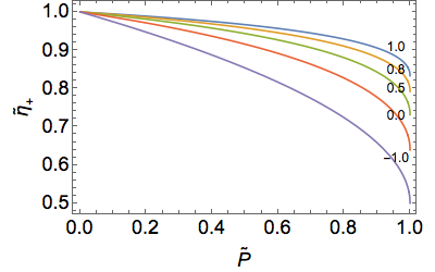
has been suggested [19], where is the normalized efficiency with the Carnot efficiency and is the dimensionless power normalized with the maximum output power . It is straightforward to show with Eq. (1) that an engine reaches the Carnot bound at zero normalized output power , and the efficiency at maximum power is recovered with , as shown in Fig. 1.
Though the analytical derivation of Eq. (1) only limited to extreme regions of and in Ref. [19], the constraint Eq. (1) works well for all the , which is checked numerically in the same reference. In this work, we give a succinct analytical derivation of this constraint in the whole region . Furthermore, we obtain a detailed constraint relation Eq. (13) which also depends on a dimensionless parameter representing the imbalance between the coupling strengths to the cold and hot heat baths. This detailed constraint relation can provide more information than Eq. (1) about how the heat engine parameters affect the upper bound of efficiency at specific output power. In the derivation, we keep temperatures of both hot and cold baths, and cycle endpoints fixed while changing only operation time.
To validate our results, we present the exact efficiency and output power of a Carnot-like heat engine with a simple two-level atom as working substance. Each point in Fig. 1 shows a particular heat engine cycle with different operation time. In this example, the evolution of engine is exactly calculated via master equation, which will be shown in the later discussion. Our model connects microscopic physical parameters in the cycle to generic parameters in many previous investigations. All points follow below our constraint curve.
II General derivation
In a finite-time heat engine cycle, we divide the heat exchange with the high () and low () temperature baths into reversible and irreversible parts, namely, , where is the irreversible entropy generated. For the reversible part, we have . The low-dissipation assumption [8, 27, 25, 26, 28, 29, 17], has been widely used in many recent studies of finite-time cycle engines, namely
| (2) |
where is the corresponding operation time. is determined by the temperature , the coupling constant to the bath, and the cycle endpoints, however, not dependent on operation time . We will show clearly its dependence on microscopic parameters in the follow example of two-level atom. The power and efficiency are obtained simply as and , where is the converted work. They can be further expressed via Eq. (2) and the fact as
| (3) | |||||
| (4) |
Applying the inequality to Eq. (3), then we obtain a simple relation between and as
| (5) |
which defines the maximum output power
| (6) |
with . We remark here the inequality Eq. (5) becomes equality only when , which directly leads to the EMP derived in Ref. [17]. This inequality results in because it reduces the right side of the equality to its infimum and all the operation times are eliminated completely. To obtain a universal constraint on efficiency and power, we should properly loose this inequality.
We notice the following fact: a convex function defined on domain satisfies
| (7) |
and If we choose the convex function as and set , , and , it is not hard to find
| (8) |
Take Eq. (8) into Eq. (3), we obtain a constraint on as
| (9) |
Thus, the total operation time is bounded by , with
| (10) |
Here, is the dimensionless power with given in Eq. (6).
In this work, we mainly concern the upper bound of the efficiency for a given power and fixed engine setup, i.e., fixed and (the lower bound is presented in Appendix A). The problem of finding the upper bound now becomes an optimization problem:
| (11) |
Because Eq. (4) is an increasing function of both and , the upper bound must be achieved under the condition . Physically, this fact can be understood as the efficiency increases as the total operation time increases. Therefore, the solution of this optimization problem is given by the condition of unique solution of Eq. (4) and . Straightforwardly, a quadratic equation for can be obtained by taking into Eq. (4):
| (12) |
The requirement of unique solution of Eq. (12) (the geometrical explanation of this requirement can be found below [Eq. (A4)] of Appendix A) is equivalent to that the discriminant of the above equation is zero. This immediately results inanother quadratic equation for , the solution of which gives the upper bound of efficiency for given power and is written explicitly as
| (13) | |||||
Here, we define a dimensionless parameter
| (14) |
which characterizes the asymmetry of the dissipation with two heat baths. In the low-dissipation region, gives the highest efficiency when the power and the heat engine setup are assigned. This upper bound is quite tight according to the simulation results (Appendix A). Moreover, in a wide region of this bound is attainable with properly chosen and , though it is not a supremum for all the .
Usually, we cannot know exactly the heat engine parameters, therefore, it is useful to find a universal upper bound for all the possible . As a function of , the analytically proof of the monotonicity of is tedious. Instead, we numerically verified that is an increasing function in the whole parameter space, see Appendix B. Thus, the overall bound is reached at , i.e. . We note that a formally similar bound was also obtained in minimal nonlinear irreversible heat engine model [19, 20]. However, the boundgiven in that model is not equivalent to Eq. (1) here. The definition of in that model is different from Eq. (6) and depends on and , which can be verified by mapping the parameters wherein back to ones in the low-dissipation model [21]. The detailed discussion can be found in Appendix C
Besides the upper bound, our method also leads to the lower bound for efficiency at arbitrary given output power,
| (15) |
The curve for lower bound is illustrated as the gray dotted curve in Fig. 1. All the simulated data with two-level atom are above this curve. The detailed derivation for the lower bound is also presented in Appendix A.
We want to emphasize here that this lower bound is different from the lower bound in [Eq. (33)] of Ref. [19]. The latter one describes the minimum value for maximum efficiency at arbitrary power, which can be derived from Eq. (13) by choosing . Yet, the lower bound we obtained in Eq. (20) determines the minimum possible efficiency for the arbitary given value of power.

To achieve the maximum efficiency at given normalized power , we adjust three parameters: the operation time and during contacting with both hot and cold baths, and the entropy generation ratio , while fixing the temperatures , , and the reversible heat exchange . The derivation leaves a question about adjusting , namely tuning and . In our previous discussion, and are phenomenological assumed without connecting to the physical parameters. In our example of two-level atomic heat engine, tuning is achieved via changing the coupling constant of heat engine to bathes. We now switch to a specific Carnot-like quantum heat engine with two-level atom.
III Validate with two-level quantum heat engine
Quantum heat engine with two-level atom is the simplest engine to illustrate the relevant physical mechanisms [30, 31]. Here, we design a Carnot-like cycle with two-level atom, whose energy levels (the excited state and ground state ) are tuned by the outsider agent to extract work, namely , where is the Pauli matrix in z-direction. The finite-time cycle consists of four strokes. Operation time per cycle is , where () is the interval of quasi-isothermal process in contact with hot (cold) bath and is the interval of adiabatic process. The quasi-isothermal process retains to the normal isothermal process at the limit . The cycle is illustrated with Fig. 2:
(i) Quasi-isothermal process in contact with hot bath (): The energy spacing change is linearly decreases as , where is the changing speed with both and fixed. The change of energy spacing is shown as solid-blue curve in Fig. 2. The linear change of the energy spacing is one of the simplest protocols.
(ii) Adiabatic process (): The energy level spacing is further reduced from to , while it is isolated from any heat bath. Since there is no transition between the two energy levels, the interval of the adiabatic process is irrelevant of the thermodynamical quantities. In the simulation, we simply use . The heat exchange is zero, and the entropy of the system remains unchanged.
(iii) Quasi-isothermal process in contact with cold bath (). The process is similar to the first process, yet the energy spacing increases with speed and ends at .
(iv) Adiabatic process (). The energy spacing is recovered to the initial value .
The two-level atom operates cyclically following the above four strokes, whose dynamics is described by the master equation
| (16) |
where is the excited state population of the density matrix , and with is the mean occupation number of bath mode with frequency . The dissipative rate is a piecewise function which is a constant () during quasi-isothermal processes (i) and (iii), and zero during the two adiabatic processes. The inverse temperature is also a piecewise function defined on quasi-isothermal processes (i) and (iii) with values and , respectively. In this work we assume the energy levels always avoid crossing during the whole cycle, thus the quantum adiabatic theorem guarantees the master equation does not involve the contribution of coherence induced by non-adiabatic transition [32, 33, 34]. In other words, the two-level quantum heat engine we study here is working in the classical regime.

In the simulation, we have chosen an arbitrary initial state, and perform the calculation of both efficiency and output power after the engine reaches a steady state, in which the final state of stroke (iv) matches the initial state of stroke (i). Different from the textbook Carnot cycle with isothermal process, the microscopic heat engine operates away from equilibrium in the finite-time Carnot-like cycle with the quasi-isothermal process. For infinite operation time , the current cycle recovers the normal Carnot cycle.
To get efficiency and power, we consider the heat exchange and work done in two quasi-isothermal processes. The internal energy change and work done in stroke (i) is and , respectively. The total heat absorbed from the hot bath is given via the first law of thermodynamics as . The same calculation can be carried out for in stroke (iii) with the initial and final times are substituted by and . The work converted and the efficiency are defined the same as in the general discussion. In our simulation, we have fixed energy spacing of the two-level atom at the four endpoints: , , , .
To check the upper bound, we have generated the efficiency and output power with different operation times. Each point in Fig. 1 corresponds to a set of different operation time . In all the simulations, the operation time and are randomly generated. All points fall perfectly under the upper bound shown in Eq. (1).
To be comparable with the general analysis above, it is meaningful to check two key conditions: (1) low-dissipation region with scaling of irreversible entropy production, and (2) the value of tuning parameters . To check the two conditions, we firstly need calculate the irreversible entropy generation. Here, we consider a generic quasi-isothermal process starts at and end at with . To simplify the discussion, we remove the index and related to the bath. The solution to Eq. (16) is formally obtained as , . The entropy change during the process is evaluated via von Neuman formula as . The irreversible entropy production in this quasi-isothermal process reads , where exchange is obtained via .
At the high temperature limit , and for , namely, the linear response region, the irreversible entropy production reads , where (see Appendix D). At long-time limit , we keep only the leading term and get the normal assumption of behavior of entropy generation
| (17) |
A general discussion about the form of the irreversible entropy generation based on stochastic thermodynamics can be found in Ref. [25]. We plot the irreversible entropy generation as a function of contacting time in Fig. 3. The points show the exact entropy generation by solving Eq. (16). At short time , the entropy deviates from the low-dissipation region. Especially, in the extremely short contact time limit, is a finite quantity instead of be divergent as in assumption. To reach this low-dissipation limit, we need either large coupling between system and bath, or long-time contacting time . In the simulation, we have chosen the operation time and to fulfill this requirement.
Back to the example of two-level atomic Carnot-like heat engine, the parameter () is simply , and is the only parameter available to the tune . Therefore, the dimensionless parameter for whole cycle can be tuned via and . In the simulation in Fig. 1, we have the parameters and . In this region the upper bound is very close the one with .
We remark that the current proof of the upper bound is based on assumption of low-dissipation. Taking the two-level atomic example, this assumption together with the microscopic expression for is guaranteed in the long time limit and with the requirement . It is interesting to note that low-dissipation can be achieved with large coupling strength , according to Eq. (17). However, it remains open to obtain the universal bound for system beyond low-dissipation region, which will be discussed elsewhere.
IV Conclusion
In summary, we have derived the constraint relation between efficiency and output power of heat engine working under the so-called low-dissipation region. A general proof of the constraint for all the region of output power is given. We also obtain a detailed constraint depending on the dissipation to the hot and cold baths, which can provide more information for a specific heat engine model. Moreover, in a concrete example of heat engine with two-level atom, we connect phenomenological parameters to the microscopic parameters, such as coupling constants to baths. These connections enable practical adjusting the heat engine to achieve the designed function via optimizing the physical parameters, and can be experimentally verified with the state of art superconducting circuit system [35].
Acknowledgements.
Y. H. Ma is grateful to Z. C. Tu, S. H. Su, and J. F. Chen for the helpful discussion. This work is supported by NSFC (Grants No. 11534002), the National Basic Research Program of China (Grant No. 2016YFA0301201 & No. 2014CB921403), the NSAF (Grant No. U1730449 & No. U1530401) and Beijing Institute of Technology Research Fund Program for Young Scholars.Appendix A Lower bound of efficiency
The lower bound is obtained via the constraint , take this equation into Eq. (3) of the main text, we have an equation of
| (18) |
This equation has only one solution
| (19) |
This solution together with Eq. (4) of the main text gives the lower bound of efficiency
| (20) |
This lower bound gives the information of the worst efficiency for a given low-dissipation heat engine at power . Similar to , is not the infimum for all the either.
As is obvious a decreasing function of , the universal lower bound is at , thus we have
| (21) |
Notice that the way we solve the lower bound is a little different from that of the upper bound. For lower bound, we directly solve the constraint with Eq. (3), instead of Eq. (4) of the main text. This can be well understood by plotting [Eq. (3) of the main text] and [Eq. (4) of the main text] on the plane spanned by and , as shown in Fig. 4. In the first quadrant, appears as the blue closed curve and as the orange open curve. The intersections of and gives the physically attainable and for given and . Two tangent lines (green dashed line) and (red dot-dashed line) sandwich in between. As is an increasing function of both and , the larger is, the curve is more away from the origin of coordinates, and vice versa. With this fact, it is not hard to see, all the curves on the right side of have larger than any possible with given. Therefore, the curve which is tangent with gives the least upper bound we can find. On the other hand, the curve itself is already on the right side for tangent line , thus the tangent point leads to the largest lower bound we can find.

To show how close the upper and lower bounds to the attainable we plot these two bounds with randomly simulated points in Fig. 5. The upper and lower bounds are calculated by Eq. (13) of the main text and Eq. (20), respectively, and the simulation points are spotted according to Eqs. (3, 4) of the main text with randomly chosen and . We can see these two bounds are quite tight that the simulated points are nearly saturate with them.


Appendix B The monotonicity of
The upper bound of efficiency is an increasing function of . As illustrated in the left panel of Fig. 6, the curves of are in the order of increasing from bottom to up. If is getting smaller, the difference of between different disappears gradually.
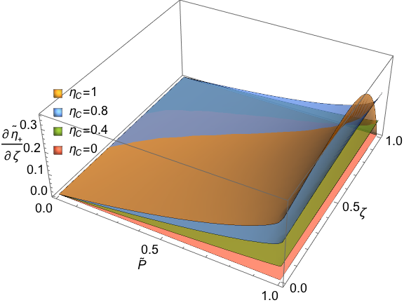
As the expression of is complicated, the analytical proof of its monotonicity is tedious and difficult. Instead numerical calculate the derivative of . As we can see in the counter plot in the right panel of Fig. 6, is non-negative in all the parameter region of and , thus is indeed an increasing function of and its maximum value is at .
Appendix C Compare with the minimally nonlinear irreversible heat engine model
Based on then extended Onsager relations, a model named as “minimally nonlinear irreversible heat engine” was proposed to study the same problem about the relation between efficiency and power. It is usually believed that the minimally nonlinear irreversible heat engine and the low-dissipation heat engine model, since there is a one-to-one mapping between the parameters of the two models [21]. Recently, a formally same constraint as Eq. (1) in the main text is obtained by the nonlinear irreversible heat engine model [20]. However, we have to emphasise that, even though there is the equivalence of the two models and the similar results they give, the bounds on efficiency at arbitrary power given by them are different. The reason can be ascribed to the optimization parameters in the two models are essentially different.
Specifically speaking, the definition of the max power in Ref. [20] is different from the one in this work. This can be verified by mapping the of Eq. (11) in Ref. [20] from the minimally nonlinear irreversible model back to the low-dissipation model. If we express the in Ref. [20] with the parameters in the low-dissipation model, it actually depends on and . Explicitly, in Ref. [20] is defined as
| (22) |
where is one of the Onsager coefficients. The mapping of the parameters of the two heat engine models is given in Ref. [21] as,
| (23) | |||||
| (24) |
In the tight-coupling case (), and with the notation , we can see the Eq. (22) reads
| (25) | |||||
which is obviously different from the max power in Eq. (6) in the main text. Therefore, Eq. (1) in this work and Eq. (22) in Ref. [20] are intrinsically different.
It can be seen from Eq. (25) that still depends on and in Ref. [20], thus another step of optimization with respect to is needed to arrive at the real max power, this fact is already indicated in the Ref. [21]. We would like to emphases here, the equivalence of the two models only means there exists a mapping between parameters of these two models, which does not imply the optimization processes and the bounds are the same.
Appendix D Irreversible entropy generation
In this section, we show detailed derivation of irreversible entropy generation of a TLA in a quasi-isothermal process. Here, we focus on the case the energy gap of the TLA is linearly changed, this minimal model is enough to illustrate the validity and limitations of the low-dissipation assumption. The more general time-dependent cases will be discussed elsewhere. The Born-Markov master equation Eq. (16) of the main text in the main text is capable of the case that the Hamiltonian has no level crossing. It can be formally solved as
| (26) |
where
| (27) |
Integrated by parts, we have
| (28) |
Here we define
which is the excited state population when the TLA is equilibrium with the heat bath. For the sake of simplification, we assume the initial state of the finite-time isothermal process is an equilibrium state, thus the last term of Eq. (28) can be ignored. Now we can discuss the high and low temperature behavior of the irreversible entropy production in such process.
D.1 High temperature limit
In the high temperature limit, , the integration in Eq. (28) is approximated as
which can be further written as, with the assumption
| (29) |
Here we define an effective dissipative rate which is in inverse of and . Therefore, in the high temperature limit the excited population reads
| (30) |
Next, the irreversible entropy production is given straightforwardly by definition,
| (31) |
The heat absorbed from the bath is given by
| (32) | |||||
and the entropy change of the system reads
| (33) | |||||
The first term of Eq. (33) is the entropy change in a quasi-static isothermal process with the same initial and final energy spacings, which can be canceled with the first three terms of Eq. (32). The last two terms of Eq. (33) are related to the entropy difference between the real finial state and the equilibrium state , the leading term of which is of the order of in the high temperature limit:
Therefore, by substituting Eqs. (32) and (33) into Eq. (31), the irreversible entropy production then reads
| (34) |
When , we keep only the leading term, thus we have
| (35) |
which is the result presented in the main text. In this minimal model, the low-dissipation assumption is valid when the operation time is longer than the time scale of . When , the irreversible entropy production has a finite limitation:
| (36) |
In this short time region, the low-dissipation assumption is not satisfied anymore, thus the constrain relation between efficiency and power discussed in the main text is not applicable in this case.
D.2 Low temperature limit
We can also obtain an approximated analytical result of the irreversible entropy production in the low temperature region . By using the fact and for low temperature, the excited state population can be approximated as
| (37) | |||||
Then the heat exchanged and the entropy change in the finite-time isothermal process are
| (38) | |||||
and
| (39) | |||||
The irreversible entropy production is straightforwardly obtained as
| (40) |
Similar as the high temperature case, the long-time behavior of is also of the form:
| (41) |
and the short time limit is also finite:
| (42) |
The low temperature irreversible entropy generation obtained by Eq. (41) is well consistent with the numerical result, as shown in Fig. 7.

References
- [1] K. Huang, Statistical Mechanics, 2nd ed. John Wiley & Sons (1987).
- [2] F. Curzon and B. Ahlborn, Am. J. Phys. 43, 22 (1975).
- [3] P. Chambadal, Les Centrales Nuclaires, 4 (Armand Colin, Paris, 1957).
- [4] I. I. Novikov, At. Energy (N.Y.) 3, 1269 (1957); J. Nucl. Energy 7, 125 (1958).
- [5] C. Van den Broeck, Phys. Rev. Lett. 95, 190602 (2005).
- [6] S. Sheng and Z. C. Tu, Phys. Rev. E 91, 022136 (2015).
- [7] K. Brandner and U. Seifert, Phys. Rev. E 91 012121 (2015).
- [8] T. Schmiedl and U. Seifert, EPL. 81, 20003 (2008).
- [9] Z. C. Tu, Phys. Rev. E. 89, 052148 (2014).
- [10] Y. Izumida and K. Okuda, EPL. 83, 60003 (2008).
- [11] Z. C. Tu, J. Phys. A 41, 312003 (2008).
- [12] A. E. Allahverdyan, R. S. Johal, and G. Mahler, Phys. Rev. E 77, 041118 (2008).
- [13] B. Rutten, M. Esposito, and B. Cleuren, Phys. Rev. B 80, 235122 (2009).
- [14] M. Esposito, R. Kawai, K. Lindenberg, and C. Van den Broeck, Phys. Rev. E 81, 041106 (2010).
- [15] I. A. Martínez, É. Roldán, L. Dinis, et. al., Nat. Phys. 12, 67 (2016).
- [16] J. Roßnagel, S. T. Dawkins, K. N. Tolazzi, et. al., Science 352, 325 (2016).
- [17] M. Esposito, R. Kawai, K. Lindenberg, and C. Van den Broeck, Phys. Rev. Lett. 105, 150603 (2010).
- [18] A. Ryabov and V. Holubec, Phys. Rev. E. 93, 050101(R) (2016).
- [19] V. Holubec and A. Ryabov, J. Stat. Mech. Theory Exp. 2016, 073204 (2016).
- [20] R. Long and W. Liu, Phys. Rev. E 94, 052114 (2016).
- [21] Y. Izumida and K. Okuda, Europhys. Lett. 97, 10004 (2012).
- [22] N. Shiraishi, K. Saito, and H. Tasaki, Phys. Rev. Lett. 117, 190601 (2016).
- [23] V. Cavina, A. Mari, and V. Giovannetti, Phys. Rev. Lett. 119, 050601 (2016).
- [24] V. Holubec and A. Ryabov, Phys. Rev. E 96, 062107 (2017).
- [25] K. Sekimoto and S. Sasa, J. Phys. Soc. Jpn. 66, 3326 (1997).
- [26] C. de Tomas, J. M. M. Roco, A. Calvo Hernández, et. al., Phys. Rev. E 87, 012105 (2013).
- [27] J. Chen, J. Phys. D: Appl. Phys. 27, 1144 (1994).
- [28] A. C. Hernández, A. Medina, and J. M. M. Roco, New J. Phys. 17, 075011 (2015).
- [29] J. Gonzalez-Ayala, A. C. Hernández, and J. M. M. Roco, J. Stat. Mech. Theory Exp. 2016, 073202 (2016).
- [30] H. T. Quan, Y. X. Liu, C. P. Sun, and F. Nori, Phys. Rev. E 76, 031105 (2007).
- [31] P. R. Zulkowski and M. R. DeWeese, Phys. Rev. E 92, 032113 (2015)
- [32] T. Albash, S. Boixo, D. A Lidar, and P. Zanardi, New J. Phys. 14, 123016 (2012).
- [33] M. Yamaguchi, T. Yuge, and T. Ogawa, Phys. Rev. E 95, 012136 (2017).
- [34] R. Dann, A. Levy, R. Kosloff, arXiv:1805.10689
- [35] F. Giazotto, T. T. Heikkilä, A. Luukanen, et. al., Rev. Mod. Phys. 78, 217 (2009).