Rayleigh-Benard convection in a hard disk system

Fluids are one of the subjects in physics that have been studied more intensively during the last centuries [2][6] [13]. Navier-Stokes (NS) equations have been the key ingredient in the understanding of observed fluid’s phenomena in nature. Their analytic and numerical solutions are, nowadays, essential to many different scenarios, from the weather prediction up to the aircrafts design. In spite of the overall success obtained by its application to practical problems, there is a lack of a rigorous connection between the underlying microscopic (typically hamiltonian) dynamics and the macroscopic NS-equations. Therefore there are still several important open issues connected to the NS main hypothesis and key ingredients used to build them. Let us mention a few of them as the local equilibrium hypothesis from which we assume that thermodynamics may be applied (up to some extend) at each macroscopic point of the fluid, the mathematical form of the transport coefficients (heat conduction and viscosities) as a function of the local fields, or the goodness of considering that the local heat conduction follows the Fourier’s law or that the stress tensor is linear on the velocity gradients (newtonian fluid). The numerous efforts that have been done so far in the NS derivation show the enormous difficulties on such task. To have some flavour on it, let us mention the nice review by Esposito et al. about the derivation of NS equations from the Boltzmann equation [11]. However, there is another way to study the connection between microscopic and macroscopic descriptions: the computer simulation tool.

We know that fluids are typically in nonequilibrium states due to the action of external agents as temperature gradients or driving fields and there appear long range correlations in space and time. Therefore it is expected that their behavior depends strongly on the boundary conditions we impose. That makes a computer simulation of a fluid a very complicated task. It is necessary a priori a very large number of particles to have a reasonable collective description of the fluid and to limit (at some extent) the effects of the details of the boundaries in the bulk system behavior. Also, the long range correlations makes very difficult to make a finite size study of the simulation by trying to extrapolate any macroscopic observable value from a sequence of measurements of it in systems with increasing number of particles. Finally, the time correlation functions are also power like which implies the need of very long runs to get a large enough set of almost independent configurations to do any observable averaging. In practice we immediately are limited by the finite power of our nowadays computers and we can use a very limited number of particles in our simulations (very far from the Avogrado’s number) from which we can get some useful data in a computation time that does not exceeds a human life span. Obviously, with such small amount of particles it is difficult to expect any reasonable connection between those simulations and the behavior described by the Navier Stokes equations. In any case, there were some attempts during the eighties with some pioneering computer simulations trying to see macroscopic hydrodynamic behavior on particle systems. Let us mention for instance the work of D.C. Rapaport and E. Clementi [26] in which they simulate a fluid flow past a cylindrical obstacle by using a set of particles with a short range pair interaction potential.

We have recently discovered [8] that a bidimensional hard disks system under the action of a temperature gradient, presents a nice property that we call boundary decoupling when studying its stationary state properties. That is, the system rearranges itself in such a way that there is a bulk part of it in which the local hydrodynamic properties hold: the local equilibrium hypothesis and the Fourier’s law. The finite size dependences are then restricted to the values of the average heat current crossing the system and the local constant pressure. In other words, for a given stationary state with measured values of the heat current and pressure, the temperature profile in the system bulk is the one corresponding to the solution of the Fourier’s law and the local temperature and density are related by the hard-disk equilibrium equation of state. We have checked this property also for a hard disk system under a shear forcing at the boundaries [9]. We want to push further the possibility to get some insight on the hydrodynamic behavior of a system by doing computer simulations. The Bénard problem is, in our opinion, the natural next problem to be studied by a computer simulation of a hard disk particle system.

The Bénard Problem consists in a fluid that is heated from below under the presence of gravity. It is observed that above some critical value of the temperature gradient the convection starts and the fluid move in rolls occupying the full system. This is the Rayleigh-Bénard instability that was observed experimentally by Bénard and afterwards there was interpreted theoretically by Rayleigh. That is, this nonequilibrium problem includes a transition from conducting to convecting states and a nonzero hydrodynamic velocity field in the convecting stationary state (see for instance some recent books and reviews in [22], [16] and [3]).

There are several papers studying the Bénard problem by using simulations of hard disks. Let us mention, for instance, the work from M. Marechal et al. [18][19] and A. Puhl et al. [23]. Mareschal and co-workers observed the transition conducting-convecting for a system of hard disks even for a very small number of particles ($N=5040$). However, the very large velocity fluctuations prevented, in that time, to get accurate measurements of local magnitudes. Nevertheless they managed to get some hydrodynamics velocity profiles that they could compare with a numerical resolution of NS equations getting a very reasonable accordance. This system was later studied also by D.C. Rapaport [27][28] showing the influence of the boundary conditions and the initial configurations on the stationary behavior of the hard disk system. Finally, let us also mention the work from D. Risso and P. Cordero in which the study the onset of the transition [30].

In this paper we show a complete set of computer simulations results whose goal is two fold: first we want to get some insights on the stationary behavior of the system and its dependence on the external parameters (gravity and temperature gradient) by observing the heat current, internal energy, pressure,… and second, we would like to check some of the basic Navier Stokes assumptions like the local equilibrium hypothesis, the Fourier’s law, the difference between the mechanical pressure versus the thermodynamic one or the efects of our system compressibility in the transition [17].

This paper is divided in several parts. Let us make a summary of the main items and results obtain on each part.

• •

  I. The physical properties of a hard system: First we introduce a catalog of known properties of a hard disks system. We do not know the equilibrium equation of state but we express all the thermodynamic equilibrium quantities as a function of it. We also derive the hydrostatic formula in equilibrium. Finally we write down the Navier Stokes equations, the general structure of the transport coefficients and their particular analytical form obtained in the Enskog approximation of the Boltzmann equation for hard disks.

• •

  II. The model: We describe the model, the dynamics of particles and the boundary conditions used in the simulation. We also discuss the election of the parameter values for the simulation. We explain how we do the local measurements of the magnitudes in order to get the hydrodynamic fields. In a computer simulation like this where the ratio between noise and signal is expected to be not small is important to do a careful analysis of errors. We explain the way we have done such analysis. Let us remark that along the paper we use an strict $3\sigma$ error interval criterion. Finally we study the relation between the averages of the magnitudes on a local region and its continuous value. That is important to have some clean scheme to define the spatial derivatives of any field.

• •

  III. Computer simulation results of equilibrium states: We check the program and the way we measure the global and local observables by doing a set of simulations at equilibrium. That is, when the temperatures on both plates are equal but maintaining the gravity field. We show that the local densities and temperatures follow accurately the theoretical results. Moreover, the local pressure measured by using the virial expression is found to give the correct results. Finally we observe that it is meaningless to measure local fluctuations of the magnitudes because they are very sensitive to the size of the local cells that in our case is certainly very small.

• •

  IV. Computer simulation results of nonequilibrium stationary states: global magnitudes. In this part we show the behavior of the global observables as a function of the temperature gradient $\Delta T$ and the intensity of the gravity field $g$. The kinetic energy per particle increases with $g$ in contrast to what happens in equilibrium and for large $\Delta T$ it grows like $\simeq\Delta T/3$ for all $g$’s. The fluctuations of the kinetic energy increase with $\Delta T$ for all $g$’s and for a fixed $\Delta T$ it increases with $g$. The interesting thing is that the fluctuations divided by the average kinetic energy to the square presents a non-monotonous behavior for a given $g$ value: starting from the equilibrium, it decreases with $\Delta T$, reaches a minimum and then it increases. As we show later in the paper, this minimum is consistent with the transition point between conducting and convecting regimes. Moreover, the critical value of the gradient at which the transition occurs increases with $g$. That behavior contrast with the one derived in the Boussinesq approximation of the Navier Stokes equations in which the critical value decreases with $g$. We explain there that the reason is that our system is compressible and then one should correct the Boussinesq assumptions accordingly.

  We also measure the hydrodynamic kinetic energy, that is, the average particle velocity on a cell, squared and summed over all cells. Obviously this magnitude should be zero in the conducting regime and non-zero in the convecting one. We obtain the transition point from the data that is consistent with other methods used in the paper. We also study the hydrodynamic kinetic energy associated with each velocity component. We observe a kind of equipartition independently of the $g$’s for large values of $\Delta T$: $e_{u,2}\simeq 3.4e_{u,1}$ where $e_{u,i}$ is the hydrodynamic kinetic energy associated to the $i$th component of the velocity.

  The Pressure is computed at the top and bottom boundaries as the moment variation of the particles when colliding with it. We observe that the global barometric formula holds always, that is the difference between the pressures at bottom and top of the system is proprotional to the system weight. This confirms the correctness of the computer simulation. Nevertheless the pressure at each boundary has a non trivial dependece on $\Delta T$ and $g$ which we analyze.

  Finally we study the energy current that cross each thermal bath boundary. We first check that the current coming into the system is exactly the same to the outgoing one. For large values of $\Delta T$ the current goes like $\Delta T^{3/2}$ for all $g$’s. In general we see that the gravity hinders the heat current for small values of $\Delta T$ while it favours it for large values of it where it correspond to the fully developed convective regime. We define a second critical thermal gradient as the one in which the thermal current for a given $g$ value equals the one when $g=0$ (pure conducting case). That is, beyond such value, convection becomes “more efficient” that conduction in transporting heat through the system for a given temperature gradient. This second critical gradient is necessary to explain some observed system behavior later in the paper.

• •

  V. Computer simulation results of nonequilibrium stationary states: spatial structures. First we study the distribution of the current line lengths for a set of stationary velocity fields. For conducting states we reasonably fit a gamma distribution to the data. In the convecting regime there is a distribution that depends on the system geometry and we analyze its form. We also analyze the fraction of velocity vectors whose modulus is larger than their standard deviation, $pr$. That is, the amount of “real” (or nonfluctuating) hydrodynamic velocity vector. We observe that this magnitude is directly correlated with the average length of the current lines in each case. Moreover, that relation is independent on the value of $g$. We see that for all $g$’s we obtain $pr\simeq 0.68$ when we are at the second critical gradient. This value coincides with the critical fraction of the covered surface at the percolation threshold of a system of overlapping disks of radius $r$. That is, the overall picture maybe that when convection begins, the current lines are small. Their length grow with the value of the thermal gradient up to a critical value in which the current lines extends and connect the system boundaries. We conclude that this phenomena is related with a percolation like transition that occurs precisely at the second critical temperature gradient.

  We study the spatial structure of the hydrodynamic velocity components. For large enough temperature gradients it seems that there is well define limiting velocity profile. Moreover we show that each hydrodynamic velocity component has an universal scaled field (universal in the sense that, once the field is scaled, it does not depend on $\Delta T$) for large enough values of $\Delta T$. The scaled field, $\tilde{u}_{1,2}(x,y)$ is obtained by

  $$\tilde{u}_{1,2}=\frac{u_{1,2}(x,y)}{\sigma(u_{1,2})}$$

  (1)

  where $u_{1,2}(x,y)$ is the components $1,2$ of the measured hydrodynamic field and $\sigma(u_{1,2})$ are their stardard deviation (the spatial average of the hydrodynamic velocity field is zero). In the process we observe the nice property: $\sigma(u_{2})=2\sigma(u_{1})$ for all fields with any $\Delta T$ and $g$ values. We study the Inertial Tensor and the fourth moment of scaled fields with different values of $\Delta T$ to look for any systematic dependence on the temperature gradient. Moreover, we compute the average mutual euclidean distance between scaled configurations to confirm that, for large enough values of $\Delta T$ such distance tends to zero. The overall analysis is lengthly because the initial data fields have non-negligible fluctuating spatial behavior and intrinsic error bars that should be taken into account to finally obtain a consistent set of results.

  We also study the Temperature field. The average $y$-profile, $\tau(y)$ is non-linear and it is convex for $g=0$ and $5$ and it has infection points for $g=10$ and $15$. We see thermal gap in the boundaries, characterize its behavior and compute the effective thermal gradient that is $\simeq 0.82\Delta T$ for all $g$-values. Finally we show also the existence of a universal scaled Temperature field that is defined by

  $$\tilde{T}(x,y)=\frac{T(x,y)-\tau(y)}{\sigma(T)}$$

  (2)

  where $\sigma(t)$ is the standard deviation with respect $\tau(y)$. In the same spirit we also analyze the density and pressure fields. In both cases we observe the existence of universal fields.

• •

  VI. Connecting with hydrodynamics. In this section we try to check some of the Navier Stokes ansatz and properties at the stationary state. Dynamic properties are beyond the scope of this article. The first thing we check is the continuity equation that express the mass conservation at the hydrodynamic level: $\nabla(\rho u)=0$ from the measured local density and velocity fields. This give us some confidence on the use of the field spatial derivatives in spite that the relative error after derivatives increases up to an average of $10\%$, large but enough to check some equation consistencies. Second we see if local equilibrium holds at each cell. We observe that it is the case for systems at the conducting regime. However we see a small and noisy systematic deviation from local equilibrium for systems at the convecting regime. We argue that it is so because of the difference between the mechanical pressure (the one we measure) and the thermodyncamic one. Their difference it is known to be proportional to the divergence of the hydrodynamic velocity. The hydrodynamic velocity divergence is small and the data is noisy but nevertheless we manage to discard the Stoke’s assumption ($\nabla u=0$) and we find that the best fit occurs when we assume that the bulk viscosity is itself dependent on the mechanical pressure. This is a weak-like result but indicates a way to go deep inside of the properties of the NS equations. Finally we check stationary NS equations for the non-convective states obtaining a reasonable good coincidence with the computer simulation results.

The overall work has been an effort to extract a coherent and systematic description of the Rayleigh-Benard problem from a microscopic computer simulation of a hard disk system. Of course there are many interesting items and observables we could study. Many of them we honestly tried to analyze (for instance local fluctuations) but we finally applied the strict criterium that anything whose error analysis obscure the average structure should be discarded. Maybe, one may focus on a particular item to design a simulation that gets much better statistics necessary to obtain with good confidence its behavior. We feel that it can be done and it is possible to study hydrodynamic behaviors from microscopic models.

Hard disks is one of the paradigmatic models in many body physics. Having a very simple dynamics it contains many nontrivial statistical properties that come from collective effects of its individuals. For instance, it has a phase transition [1] or its time correlation functions have the long time tails [33]. Moreover its exact Equation of State (EOS) is not yet derived in the context of the equilibrium statistical physics [21]. Let us state some basic properties that are known and that we are going to use during the computer simulation data analysis.

• •

  Equilibrium properties: The canonical partition function for a system with $N$ disks with mass $m$ and radius $r$ enclosed in a box of sides $L_{x}$ an $L_{y}$ at a temperature $T$ is given by

  $$Z(N,S,T)=\frac{1}{h^{2N}N!}\left(2\pi mk_{B}T\right)^{N}Z_{c}(N,S)$$

  (3)

  where $S$ is the box surface ($S=L_{x}L_{y}$) and $Z_{c}$ is the configurational partition function that, in the hard disk case, it doesn’t depend on the temperature. $Z_{c}$ is not known but it can be connected with the equation of state that has been extensively studied numerically and very good analytical expressions have been derived from the extensive computer simulations [21]. The equation of state for a hard disk system has the general form:

  $$PS=Nk_{B}TH(\rho)\quad,\quad\rho=\frac{N\pi r^{2}}{S}$$

  (4)

  A well known simple form for $H$ was proposed by Henderson [15] that fits very well the data for de areal density interval $\rho\in[0,0.5]$:

  $$H(\rho)=\frac{1+\rho^{2}/8}{(1-\rho)^{2}}$$

  (5)

  The equation of state is connected with $Z_{c}$ by the expression:

  $$P=k_{B}T\frac{\partial Z_{c}}{\partial S}\quad\Rightarrow\quad NH(\rho)=-\rho\frac{\partial Z_{c}}{\partial\rho}$$

  (6)

  If we assume that $Z_{c}\simeq\exp[N\bar{f}(\rho)]$ for $N$ large enough, we obtain:

  $$\bar{f}(\rho)=\bar{f}(\rho^{*})-\int_{\rho^{*}}^{\rho}d\tilde{\rho}\,\,\frac{H(\tilde{\rho})}{\tilde{\rho}}$$

  (7)

  where $\rho^{*}$ is any arbitrary value. We know that in the limit $\rho\rightarrow 0$ the hard disk system behaves like an ideal gas. In such limit $f(0)=\ln S$, substituting $\rho^{*}=0$ above we get

  $$\bar{f}(\rho)=\frac{1}{N}lnZ_{c}=ln\left(\frac{\pi r^{2}N}{\rho}\right)-\int_{0}^{\rho}d\tilde{\rho}\,\,\frac{H(\tilde{\rho})-1}{\tilde{\rho}}$$

  (8)

  and the hard disk partition function can be written for $N$ large:

  $$Z\simeq e^{Nf(\rho)}\quad\quad,\quad f(\rho)=ln\frac{T}{\rho}-\int_{0}^{\rho}d\tilde{\rho}\,\,\frac{H(\tilde{\rho})-1}{\tilde{\rho}}+C$$

  (9)

  where $C$ is the constant

  $$C=ln\left(\frac{2mk_{B}e\pi^{2}r^{2}}{h^{2}}\right)$$

  (10)

  From it we can compute all thermodynamic magnitudes, for example, the entropy is given by

  $$\frac{s}{k_{B}}=f(\rho)+1$$

  (11)

  the specific heats at constant pressure and volume are respectively

  $$\frac{c_{P}}{k_{B}}=1+\frac{H(\rho)^{2}}{H(\rho)+\rho\frac{dH(\rho)}{d\rho}}\quad,\quad c_{V}=k_{B}$$

  (12)

  and the coefficients $\alpha$ and $\kappa_{T}$ are

  $$\alpha=\frac{1}{T}\frac{H(\rho)}{H(\rho)+\rho\frac{dH(\rho)}{d\rho}}\quad,\quad\kappa_{T}=\frac{\pi r^{2}}{k_{B}T\rho}\frac{1}{H(\rho)+\rho\frac{dH(\rho)}{d\rho}}$$

  (13)

• •

  Hard disks under the action of an external field at equilibrium: the hydrostatic formula

  Let us assume now that over the hard disk system, there is an external field acting on the particles. That is, we should add to the Hamiltonian a term of the form:

  $$H_{ext}=\sum_{i=1}^{N}U(\vec{r}_{i})$$

  (14)

  Then, to obtain the equilibrium properties it is convenient to use the grand canonical ensemble. The computation simplifies if we consider a very slow varying external field (we follow here the arguments in Martin-Lof’s book [20]). That is, $U(\vec{r})=\tilde{U}(\vec{r}/L)$ being $\tilde{U}$ a smooth function in $R^{2}$. We can define a box with a volume that grows with $L^{2}$ at a given position $\vec{x}$. When $L\rightarrow\infty$ the particles of the bulk of the box only see an external constant field of value $\tilde{U}(\vec{x})$ and then $H_{ext}=N\tilde{U}(\vec{x})$. The local thermodynamic properties of the system can be computed using the grand canonical ensemble just substituting the chemical potential $\mu\rightarrow\mu-\tilde{U}(\vec{x})$. For instance, the equation of state is given in a parametric form:

  	$\displaystyle P$	$\displaystyle=$	$\displaystyle k_{B}Ta(T,\mu-\tilde{U}(\vec{x}))$
  	$\displaystyle\tilde{\rho}$	$\displaystyle=$	$\displaystyle k_{B}T\frac{d}{d\mu}a(T,\mu-\tilde{U}(\vec{x}))$

  where $\tilde{\rho}$ is the particle density, $a=a(T,\mu)=\lim_{S\rightarrow\infty}S^{-1}\log{\mathcal{Z}}$ and ${\mathcal{Z}}$ is the gran canonical partition function. We can eliminate the parameter $\mu$ by applying the gradient to the pressure and using the definition of $\tilde{\rho}$. Thus, we obtain the hydrostatic formula:

  $$\nabla P=-\tilde{\rho}(\vec{x})\nabla\tilde{U}$$

  (15)

  Notice that the full argument is general and it is not restricted to a hard disk system.

• •

  Navier-Stokes Equations for hard disk systems:

  Navier Stokes equations describe the dynamics of a macroscopic fluid [13] and they are constructed assuming: (1) the local conservation of density, linear momentum and energy, (2) the local equilibrium property and (3) some local constitutive relations (Fourier’s law, Newtonian fluid). The macroscopic evolving fields are: the local mass density, $\tilde{\rho}(x,t)$, the local velocity components, $u_{i}(x,t)\,,\,i=1,\ldots,d$, and the local temperature, $T(x,t)$. Their evolution is determined by:

  	$\displaystyle\partial_{t}\tilde{\rho}+\sum_{i}\partial_{i}(\tilde{\rho}u_{i})$	$\displaystyle=$	$\displaystyle 0$
  	$\displaystyle\partial_{t}u_{i}+\sum_{j}u_{j}\partial_{j}u_{i}$	$\displaystyle=$	$\displaystyle\frac{1}{\tilde{\rho}}\sum_{j}\partial_{j}\tau_{ij}+g_{i}\quad(i=1,\ldots,d)$
  	$\displaystyle\tilde{\rho}\tilde{c}_{v}\left(\partial_{t}T+\sum_{i}u_{i}\partial_{i}T\right)$	$\displaystyle=$	$\displaystyle-T\frac{\partial P}{\partial T}\biggr|_{\tilde{\rho}}\sum_{i}\partial_{i}u_{i}+\sum_{ij}\tau^{\prime}_{ij}\partial_{i}u_{j}+\sum_{ij}\partial_{i}\left(\kappa_{ij}\partial_{j}T\right)$		(16)

  Assuming that we study the so called newtonian fluids then:

  	$\displaystyle\tau_{ij}$	$\displaystyle=$	$\displaystyle-P\delta_{ij}+\tau^{\prime}_{ij}$
  	$\displaystyle\tau^{\prime}_{ij}$	$\displaystyle=$	$\displaystyle\eta\left(\partial_{i}u_{j}+\partial_{j}u_{i}\right)+\eta^{\prime}\delta_{ij}\sum_{k}\partial_{k}u_{k}$		(17)

  Finally, the local equilibrium property also implies that the equilibrium equation of state applies to the local fields: $P=P(\tilde{\rho},T)$. Observe that we also need to know the equilibrium mass specific heat at constant volume $\tilde{c}_{v}=\tilde{c}_{v}(\tilde{\rho},T)$ and the transport coefficient functions: the thermal conductivity $\kappa=\kappa(\tilde{\rho},T)$, the shear viscosity $\eta=\eta(\tilde{\rho},T)$ and the second viscosity $\eta^{\prime}=\eta^{\prime}(\tilde{\rho},T)$ . All these equations plus the value of the external field $g_{i}$ and the boundary conditions for the fields give us a complete description of the evolution of a fluid at the macroscopic level.

  For hard disks system we know the EOS and then

  $$\frac{\partial P}{\partial T}\biggr|_{\tilde{\rho}}=\frac{P}{T}$$

  (18)

  and $c_{v}=k_{B}$. Notice that $\rho=N\pi r^{2}/L_{x}L_{y}$ and it is related to the mass density by: $\tilde{\rho}=m\rho/\pi r^{2}$ where $m$ is the mass of one disk and $r$ its radius.

  Moreover one can show that the transport coefficients have also a simple dependence on the temperature:

  	$\displaystyle\eta$	$\displaystyle=$	$\displaystyle\frac{\sqrt{k_{B}m}}{r}\sqrt{T}E(\rho)$
  	$\displaystyle\eta^{\prime}$	$\displaystyle=$	$\displaystyle\frac{\sqrt{k_{B}m}}{r}\sqrt{T}E^{\prime}(\rho)$
  	$\displaystyle\kappa$	$\displaystyle=$	$\displaystyle\frac{\sqrt{k_{B}^{3}}}{r\sqrt{m}}\sqrt{T}K(\rho)$		(19)

  We are going to be interested on the stationary solutions when the external field is $g_{j}=-g\delta_{j,2}$. The resulting equations after we substitute these formulas into eqs. (16) are:

  	$\displaystyle\partial_{1}(\rho u_{1})+\partial_{2}(\rho u_{2})$	$\displaystyle=$	$\displaystyle 0$		(20)
  	$\displaystyle\rho\left(u_{1}\partial_{1}u_{1}+u_{2}\partial_{2}u_{1}\right)$	$\displaystyle=$	$\displaystyle-\partial_{1}Q+\pi r\partial_{1}\left[\sqrt{T}\left(2E\partial_{1}u_{1}+E^{\prime}(\partial_{1}u_{1}+\partial_{2}u_{2})\right)\right]$		(21)
  		$\displaystyle+$	$\displaystyle\pi r\partial_{2}\left[\sqrt{T}E\left(\partial_{1}u_{2}+\partial_{2}u_{1}\right)\right]$
  	$\displaystyle\rho\left(u_{1}\partial_{1}u_{2}+u_{2}\partial_{2}u_{2}\right)$	$\displaystyle=$	$\displaystyle-\partial_{2}Q+\pi r\partial_{2}\left[\sqrt{T}\left(2E\partial_{2}u_{2}+E^{\prime}(\partial_{1}u_{1}+\partial_{2}u_{2})\right)\right]$		(22)
  		$\displaystyle+$	$\displaystyle\pi r\partial_{1}\left[\sqrt{T}E\left(\partial_{1}u_{2}+\partial_{2}u_{1}\right)\right]-\rho g$
  	$\displaystyle\rho\left(u_{1}\partial_{1}T+u_{2}\partial_{2}T\right)$	$\displaystyle=$	$\displaystyle-Q(\partial_{1}u_{1}+\partial_{2}u_{2})+2\pi r\sqrt{T}E\left((\partial_{1}u_{1})^{2}+(\partial_{2}u_{2})^{2}\right)+\pi r\sqrt{T}E^{\prime}\left(\partial_{1}u_{1}+\partial_{2}u_{2}\right)^{2}$		(23)
  		$\displaystyle+$	$\displaystyle\pi r\sqrt{T}E\left(\partial_{1}u_{2}+\partial_{2}u_{1}\right)^{2}+\pi r\left[\partial_{1}\left(\sqrt{T}K\partial_{1}T\right)+\partial_{2}\left(\sqrt{T}K\partial_{2}T\right)\right]$

  where we have defined the reduced pressure, $Q=\pi r^{2}P$, and let us remind that $E$, $E^{\prime}$ and $K$ are functions of $\rho$. We have also done, after the computation, the following mapping:

  $$k_{B}T\rightarrow T\quad,\quad mg\rightarrow g\quad,\quad\sqrt{m}u_{1,2}\rightarrow u_{1,2}$$

  (24)

  With this mapping the equation of state is:

  $$Q=TF(\rho)=T\rho H(\rho)$$

  (25)

  Observe that we use in all the equation the areal density $\rho$ instead the mass density $\tilde{\rho}$.

  The NS equations for hard disks simplify when looking for non-convective stationary solutions:

  $$\rho=\rho^{NC}(y)\quad,\quad u_{x}=u_{y}=0\quad,\quad T=T^{NC}(y)$$

  (26)

  that are solutions of:

  	$\displaystyle\frac{dQ^{NC}}{dy}$	$\displaystyle=$	$\displaystyle-g\rho^{NC}$		(27)
  	$\displaystyle\sqrt{T}K(\rho^{NC})\frac{dT^{NC}}{dy}$	$\displaystyle=$	$\displaystyle-J$		(28)
  	$\displaystyle Q^{NC}$	$\displaystyle=$	$\displaystyle T^{NC}F(\rho^{NC})$		(29)

  with the boundary conditions:

  $$T(0)=T_{0}\quad,\quad T(1)=T_{1}=1\quad,\quad\bar{\rho}=\int_{0}^{1}dy\rho^{NC}(y)$$

  (30)

  where $T_{0}$, $g$ and $\bar{\rho}$ are the control parameters. Observe that $J$ is a constant that it is be obtained as a function of the external parameters.

• •

  Transport coefficients (in the Enskog approximation): Gass computed the transport coefficients for the hard disk system in the Enskog approximation [14]. The shear viscosity $\eta$, the bulk viscosity $\xi$ and the thermal conductivity $\kappa$ are:

  	$\displaystyle\eta$	$\displaystyle=$	$\displaystyle\frac{\sqrt{k_{B}m}}{r}\sqrt{T}E(\rho)\quad,\quad E(\rho)=\frac{0.255}{\sqrt{\pi}\chi(\rho)}\left[1+2\rho\chi(\rho)+3.4197\rho^{2}\chi(\rho)^{2}\right]$
  	$\displaystyle\xi$	$\displaystyle=$	$\displaystyle\frac{\sqrt{k_{B}m}}{r}\sqrt{T}E_{B}(\rho)\quad,\quad E_{B}(\rho)=1.2734\rho^{2}\chi(\rho)$
  	$\displaystyle\kappa$	$\displaystyle=$	$\displaystyle\frac{\sqrt{k_{B}^{3}}}{r\sqrt{m}}\sqrt{T}K(\rho)\quad,\quad K(\rho)=\frac{1.029}{\chi(\rho)}\left[1+3\rho\chi(\rho)+3.4874\rho^{2}\chi(\rho)^{2}\right]$		(31)

  where

  $$\chi(\rho)=\frac{H(\rho)-1}{2\rho}$$

  (32)

  and the second viscosity $\eta^{\prime}=\xi-\eta$.

Our system is composed of a set of $N$ hard disk particles that move in a square box of side $L=1$. Each disk have unit mass ($m=1$) and its radius ($r$) is chosen such that the areal density is $\bar{\rho}=N\pi r^{2}/L^{2}$, that is $r=(\bar{\rho}L^{2}/(N\pi))^{1/2}$. The dynamics of a given disk has two parts: (1) free flight and (2) collisions.

(1) Free fligth: Between collisions each disk $i$ is under the unique action of a constant external field $\vec{a}=(0,-g)$. Thus, its equations of motion are given by

whose trivial solutions are

where $\vec{r}_{i}(0)$ and $\vec{v}_{i}(0)$ are the values of the disk position and velocity after a collision of the disk has taken place.

(2) Collisions: A disk have three types of collisions, with another disk, with the box vertical boundaries and with the box horizontal boundaries. (a) Two disks collide when their distance equals $2r$. When it happens, the linear moment and the kinetic energy is conserved and it is assumed that the velocity components perpendicular to the vector that joints the centers of the disks keep unaltered during the collision. That is, we do not consider the existence of disk internal rotation around its center. (b) When the disk collides with a vertical side of the box at $x=0$ or $x=1$ it gets perfectly reflected, that is $v_{1}\rightarrow-v_{1}$ and $v_{2}\rightarrow v_{2}$. (c) when the disk hits a horizontal boundary at $y=0$ or $y=1$ the disks changes its second component of its velocity by getting a random value chosen from a Maxwellian distribution with temperature $T_{0}$ or $T_{1}$ when hitting at $y=0$ or $y=1$ respectively. That is $v_{1}\rightarrow v_{1}$ and $v_{2}\rightarrow v_{2}=s_{0,1}(-2T_{0,1}\log(1-\xi))$ being $\xi$ an uniform random variable between $[0,1]$ and $s_{0}=1$ and $s_{1}=-1$.

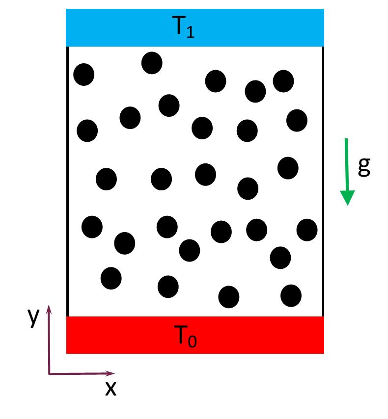
Initially the disks are placed regularly on the box with a random initial velocity vector with a modulus that is the square root of the sum of the two thermal bath temperatures. We evolve the system during $5\times 10^{4}$ collisions per particle ($\simeq 5\times 10^{7}$ collisions) when we check that the system is in the stationary state. Then we begin to take measures of different observables each $100$ collisions per particle. The simulation extends during $10^{7}$ collisions per particle ($\simeq 10^{10}$ total number of collisions) and we obtain $M=10^{5}$ data for averaging. The observables have typical errors of $3\sigma/\sqrt{M}\simeq 0.01\sigma$ that is sufficient to analyze with some detail many of their interesting behavior.

Computer simulations of hard disks systems have many advantages. First, the intrinsic dynamics is very symple and it can be implemented in the computer with very high efficiency without any loss of precision (see for instance [7][29]). Moreover, its purely kinetic structure makes possible to fix one of the system external parameters $(T_{0},T_{1},g)$ by just a time rescaling. In other words: If we rescale time, $t=\alpha t^{\prime}$, the particle velocities rescale by $v=v^{\prime}/\alpha$ and then, choosing the temperature of the thermal baths being $T^{\prime}_{0,1}=\alpha^{2}T_{0,1}$ and the gravity field $g^{\prime}=\alpha^{2}g$, the dynamic evolution of the system with parameters $(T_{0},T_{1},g)$ is indistinguishable from the one with parameters $(T_{0}^{\prime},T_{1}^{\prime},g^{\prime})$. We can arbitrarily choose $\alpha=1/\sqrt{T}_{1}$ in order to fix to one the temperature of the the thermal bath at top. Therefore we can do the simulations varying only two parameters $(T_{0}^{\prime},T_{1}^{\prime}=1,g^{\prime})$. In order to obtain the behavior of any observable for an arbitrary value of $T_{1}$ we just should undo the corresponding time rescale on the variables defining the magnitude.

In order to choose the set of values for the parameters $\bar{\rho}$ (the average areal density), $T_{0}$ and $g$ we should pay attention to the phenomena we want to describe. In this case we would like to study the transient from non-convective regime to the convective one. Then it is reasonable to use the Rayleigh coefficient ($Ra$) that is a non-dimensional magnitude that localizes the parameter regions where the fluid is in a convective/non-convective state. It is defined by

where $g$ is the intensity of the external field, $\Delta T=T_{0}-T_{1}$, $\nu=\eta/\tilde{\rho}$ is the kinematic viscosity, $\bar{\kappa}=\kappa/\tilde{\rho}\tilde{C}_{P}$ and $\tilde{\rho}=m\rho/\pi r^{2}$ is the mass density and $C_{P}=c_{p}/m$ is the specific heat capacity per unit mass.

For a hard disks case it is known that linearizing NS equations under the Boussinesq approximation there is a critical Rayleigh number $Ra_{c}=27\pi^{4}/4\simeq 657.51$ for the stress free boundary condition case (see for instance S. Chandrasekhar [6]). Convection appears when the system has a Rayleigh number above the critical value.

We have computed $Ra$ by using the Henderson equation of state and the Enskog transport coefficients. We choose the number of particles to be small enough to have a very fast system evolution to get the largest quantity of data to average. One may think that $N$ small would implies very large finite size effects. However, we already shown in previous studies with hard disks [8] that the system have a boundary decoupling property in which the system re adapts its bulk configuration to behave as it was an infinite system with effective boundary conditions composed by the ones we define in the simulation plus a small region with disks around them. For the computer simulation in this paper we chose $N=957$.

In figure 2 we show $Ra$ computed using the Enskog transpot coefficients and the Henderson equation of state. In figure 2 left we see the behavior of $Ra$ for $T_{0}=5$ for different values of $g=5$, $10$ and $15$. We see that the maximum value of $Ra$ apears for low densities and it is above the critical Rayleigh number. Then, we have chosen that the average system density to be $\bar{\rho}=0.2$. Figure 2 right we plot $Ra$ as a function of $T_{0}$ for fix $\bar{\rho}=0.2$ to have some idea of the critical value of $T_{0}$ that separates non-convective to convective regimes. We get the following critical temperatures: $T_{0}^{c}(g=5)=1.6205$, $T_{0}^{c}(g=10)=1.2233$ and $T_{0}^{c}(g=15)=1.1376$ . That is, when we increase the external field, the convective regime appears for lower temperatures.

From now on we will call to the simulated parameters $(T_{0},T_{1}=1,g)$ whose chosen values are: $g=0$, $5$, $10$ and $15$, and $T_{0}=1,1.2,1.4,1.6,1.8,2.0,2.2,2.4,2.6,2.8,3,4,\ldots,19,20$. That is, we have done $112$ computer simulations.

Before begining the analysis of the data we have obtained let us make some comments about notation, how the measurements have been done and the error bars criteria we have used.

• •

  Notation: In general a vector $u$ have two components $u=(u_{1},u_{2})$. In order to do local measurements, we divide the unit box into $30\times 30$ (virtual) square cells of side $1/30$. A given cell has the position $(n,l)$ with $n,l=1,\ldots,30$. We express hydrodynamic magnitudes at a given macroscopic point $(x,y)$ with $x,y\in[0,1]$ that correspond to the values measured of some microscopic observable at the cell $(n,l)$ such that $x=(n-1)/30+1/60$ and $y=(l-1)/30+1/60$. That is, we use the center of each cell as the macroscopic position of the hydrodynamic fields. Finally, a macroscopic hydrodynamic field is written as $u=(u_{1}(x,y),u_{2}(x,y))$

• •

  Local Measurements: The local measurements have been done in the following way. Let $a(r,v)$ be a magnitude that depend on a set of particle positions and velocities $r_{i}$ and $v_{i}$ respectively. Say for instance the kinetic energy of a particle: $a(r_{i},v_{i})=v_{i}^{2}/2=(v_{i,1}^{2}+v_{i,2}^{2})/2$ or the local potential energy of a particle: $a(r_{i},v_{i})=gr_{i,2}$ where $r_{i}=(r_{i,1},r_{i,2})$. The extensive value of $a(r,v)$ on the cell $(n,l)$ ($n,l=1,\ldots,30$) at time $t$ is given by:

  $$A(n,l;t)=\sum_{i:r_{i}(t)\in B(n,l)}a(r_{i}(t),v_{i}(t))$$

  (35)

  where $B(n,l)$ is the spatial domain corresponding to the cell $(n,l)$. The total number of particles involved in such sum is given by:

  $$N(n,l;t)=\sum_{i:r_{i}(t)\in B(n,l)}1$$

  (36)

  We do $M$ measurement of $A(n,l;t)$ during the system evolution at the stationary state. Then the average value per particle of $A$ is given by:

  $$a(n,l)=\frac{\sum_{t=1}^{M}A(n,l;t)}{\sum_{t=1}^{M}N(n,l;t)}$$

  (37)

  We use this method because it has a better convergence to the limiting value when $M\rightarrow\infty$ and its fluctuations are smaller than in case we averaged $A(n,l;t)/N(n,l;t)$ over time.

• •

  Analysis of errors: Let $\{A(t)\}_{t=1}^{M}$ the set of $M$ measurements of a given observable (local or global one). We assume that the data sequence is time decorrelated and then the law of large numbers apply. That is, the averaged value of $A$ behaves for large $M$ values as:

  $$A(M)\simeq A(\infty)+\sigma(A;M)\xi$$

  (38)

  where

  $$A(M)=\frac{1}{M}\sum_{t=1}^{M}A(t)\quad\quad,\quad\sigma(A;M)=\frac{1}{M}\sqrt{\sum_{t=1}^{M}(A_{t}-A(M))^{2}}$$

  (39)

  and $\xi$ is a Gaussian random variable with zero mean and variance one. In this paper the error in getting the $M\rightarrow\infty$ value is given by

  $$A(\infty)=A(M)\pm 3\sigma(A;M)$$

  (40)

  that is, we are assuming that the $99.7\%$ of the data is in the error interval we show in the analysis.

  Sometimes, once we have computed the average value of the observable $A$ and its error, we need to study a function of it, say $f(A)$. Let us assume that the error is small and It can be considered as a perturbation of $A(\infty)$, then we can do a Taylor expansion:

  $$f(A(M))=f(A(\infty)+\sigma(A;M)\xi)=f(A(\infty))+f^{\prime}(A(\infty))\sigma(A;M)\xi+\frac{1}{2}f^{\prime\prime}(A(\infty))\sigma(A;M)^{2}\xi^{2}+\ldots$$

  (41)

  If we average this expression over the random values $\xi$ we obtain that $\langle f(A(M))\rangle=f(A(\infty))+\frac{1}{2}f^{\prime\prime}(A(\infty))\sigma(A;M)^{2}$. There is a small but systematic shift on the observed value $f(A(M))$ with respect the desired $f(A(\infty))$. Let us define the observable:

  $$B=f(A(M))-\frac{1}{2}f^{\prime\prime}(A(\infty))\sigma(A;M)^{2}$$

  (42)

  Obviously the average value of $B$ is $f(A(\infty))$ (by construction) up to order $\sigma^{4}$ and the variance of $B$ is:

  	$\displaystyle\sigma(B)^{2}$	$\displaystyle=$	$\displaystyle\langle(B-f(A(\infty)))^{2}\rangle=\langle\left(f^{\prime}(A(\infty))\sigma(A;M)\xi+\frac{1}{2}f^{\prime\prime}(A(\infty))\sigma(A;M)^{2}(\xi^{2}-1)\right)^{2}\rangle$		(43)
  		$\displaystyle=$	$\displaystyle\sigma(A;M)^{2}\left[f^{\prime}(A(\infty))^{2}+\frac{1}{2}f^{\prime\prime}(A(\infty))^{2}\sigma(A;M)^{2}\right]$

  The error in computing $B$ is then $B=f(A(\infty))\pm 3\sigma(B)$ and we conclude that

  $$f(A(\infty))=f(A(M))-\frac{1}{2}f^{\prime\prime}(A(\infty))\sigma(A;M)^{2}\pm 3\sigma(B)$$

  (44)

  Typically the systematic shift is smaller than the error interval and therefore not relevant for the analysis. However, sometimes we obtain small but positive data values for an observable that one knows that it should be zero in average and we should introduce this correction in order to do a correct data analysis.

  Let us consider another typical case: when we compute an observable as an spatial average of local observables with their own error. That is, let $A(x,y)$ a local observable with errors $\epsilon(x,y)$. Let

  $$B=\frac{1}{N_{C}}\sum_{(x,y)}A(x,y)$$

  (45)

  If we assume that the local random variables $\xi(x,y)$ associated to the errors $\epsilon(x,y)$ are spatially independent, then we can apply the Lyapunov Central Limit Theorem (see Appendix I) and the error of $B$ is given by:

  $$\epsilon(B)=\frac{1}{N_{C}}\left[\sum_{(x,y)}\epsilon(x,y)^{2}\right]^{1/2}$$

  (46)

  Notice that the assumption of spatial independence is not so obvious because the fluid has typically long range correlations that should affect to the data noise behavior.

  However, let us assume that the data error is totally correlated in the sense that the local random variable can be written as $\xi(x,y)=\epsilon(x,y)\xi$ where $\xi$ is now a Gaussian noise with zero mean and variance one. In this case the error of $B$ is given by:

  $$\epsilon(B)=\frac{1}{N_{C}}\sum_{(x,y)}\epsilon(x,y)$$

  (47)

  Observe that the totally correlated case has an error much larger that the uncorrelated one. It is not clear a priori what scheme to choose to define errors in this case without computing the data correlation function that it is very costly from a computational point of view. In any case the true error on $B$ would have a value in between of the two limiting cases.

• •

  Differences between Local values and cell averages:

  To obtain local values of an observable we have build a set of virtual cells where we have measured the desired magnitudes. That is an arbitrary choice and we could define other partition and associate a value of the magnitude on each of its elements. Therefore we can assume that at the stationary state, for each microscopic observable, there exists a function defined in ${\mathcal{R}}^{2}$ such that its averages over any partition is the value measured on the cell. In other words:

  $$\tilde{F}(m,n)=\frac{1}{\Delta^{2}}\int_{\tilde{x}(m,n)-\Delta/2}^{\tilde{x}(m,n)+\Delta/2}dx\int_{\tilde{y}(m,n)-\Delta/2}^{\tilde{y}(m,n)+\Delta/2}dy\,F(x,y)$$

  (48)

  where $\tilde{F}(m,n)$ is the average value of the observable that we obtain in the computer simulation and $F(x,y)$ its, assumed existing, underlying continuum density. We consider that $\tilde{x}(m,n)=(m-1/2)\Delta$, $\tilde{y}(m,n)=(n-1/2)\Delta$ where $\Delta=1/N_{C}$ and $m,n=1,\ldots,N_{C}$ ($N_{C}=30$ in our computer simulations). The question that arises is what is the relation between this local averages and the value of $F$ and its derivatives at the point $(\tilde{x}(m,n),\tilde{y}(m,n))$. In order to find such relations let us write the value of $\tilde{F}$ for neighboring cells:

  $$\tilde{F}(m+s,n+t)=\frac{1}{\Delta^{2}}\int_{\tilde{x}(m,n)+s\Delta-\Delta/2}^{\tilde{x}(m,n)+s\Delta+\Delta/2}dx\int_{\tilde{y}(m,n)+t\Delta-\Delta/2}^{\tilde{y}(m,n)+t\Delta+\Delta/2}dy\,F(x,y)$$

  (49)

  We can expand the last expression assuming that $F$ is analytic and $\Delta$ is small enough, then:

  	$\displaystyle\tilde{F}(m+s,n+t)$	$\displaystyle=$	$\displaystyle\sum_{n^{\prime}=0}^{\infty}\Delta^{2n^{\prime}}\sum_{k^{\prime}=0}^{n^{\prime}}F_{(2k^{\prime},2n^{\prime}-2k^{\prime})}(m,n)a(s,k)a(t,n^{\prime}-k^{\prime})$		(50)
  		$\displaystyle+$	$\displaystyle\sum_{n^{\prime}=0}^{\infty}\Delta^{2n^{\prime}+2}\sum_{k^{\prime}=0}^{n^{\prime}}F_{(2k^{\prime}+1,2n^{\prime}-2k^{\prime}+1)}(m,n)b(s,k)b(t,n^{\prime}-k^{\prime})$
  		$\displaystyle+$	$\displaystyle\sum_{n^{\prime}=0}^{\infty}\Delta^{2n^{\prime}+1}\sum_{k^{\prime}=0}^{n^{\prime}}F_{(2k^{\prime}+1,2n^{\prime}-2k^{\prime})}(m,n)b(s,k)a(t,n^{\prime}-k^{\prime})$
  		$\displaystyle+$	$\displaystyle\sum_{n^{\prime}=0}^{\infty}\Delta^{2n^{\prime}+1}\sum_{k^{\prime}=0}^{n^{\prime}}F_{(2k^{\prime},2n^{\prime}-2k^{\prime}+1)}(m,n)a(s,k)b(t,n^{\prime}-k^{\prime})$

  where $F_{(n^{\prime},l^{\prime})}(m,n)=\partial_{x}^{n^{\prime}}\partial_{y}^{l^{\prime}}F(x,y)|_{\tilde{x}(m,n),\tilde{y}(m,n))}$ and

  	$\displaystyle a(s,l)$	$\displaystyle=$	$\displaystyle\sum_{k=0}^{l}\frac{1}{(2k)!(2l-2k+1)!}\frac{s^{2k}}{2^{2l-2k}}$
  	$\displaystyle b(s,l)$	$\displaystyle=$	$\displaystyle\sum_{k=0}^{l}\frac{1}{(2k+1)!(2l-2k+1)!}\frac{s^{2k+1}}{2^{2l-2k}}$

  Observe that $a(-s,l)=a(s,l)$ and $b(-s,l)=-b(s,l)$. These symmetry properties allows us to break eq. (50) in a set of four equations:

  	$\displaystyle G_{1}(m,n;s,t)$	$\displaystyle\equiv$	$\displaystyle\frac{1}{4}\left[\tilde{F}(m+s,n+t)+\tilde{F}(m+s,n-t)+\tilde{F}(m-s,n+t)+\tilde{F}(m-s,n-t)\right]$
  		$\displaystyle=$	$\displaystyle\sum_{n^{\prime}=0}^{\infty}\Delta^{2n^{\prime}}\sum_{k^{\prime}=0}^{n^{\prime}}F_{(2k^{\prime},2n^{\prime}-2k^{\prime})}(m,n)a(s,k)a(t,n^{\prime}-k^{\prime})$
  	$\displaystyle G_{2}(m,n;s,t)$	$\displaystyle\equiv$	$\displaystyle\frac{1}{4}\left[\tilde{F}(m+s,n+t)-\tilde{F}(m+s,n-t)-\tilde{F}(m-s,n+t)+\tilde{F}(m-s,n-t)\right]$
  		$\displaystyle=$	$\displaystyle\sum_{n^{\prime}=0}^{\infty}\Delta^{2n^{\prime}+2}\sum_{k^{\prime}=0}^{n^{\prime}}F_{(2k^{\prime}+1,2n^{\prime}-2k^{\prime}+1)}(m,n)b(s,k)b(t,n^{\prime}-k^{\prime})$
  	$\displaystyle G_{3}(m,n;s,t)$	$\displaystyle\equiv$	$\displaystyle\frac{1}{4}\left[\tilde{F}(m+s,n+t)+\tilde{F}(m+s,n-t)-\tilde{F}(m-s,n+t)-\tilde{F}(m-s,n-t)\right]$
  		$\displaystyle=$	$\displaystyle\sum_{n^{\prime}=0}^{\infty}\Delta^{2n^{\prime}+1}\sum_{k^{\prime}=0}^{n^{\prime}}F_{(2k^{\prime}+1,2n^{\prime}-2k^{\prime})}(m,n)b(s,k)a(t,n^{\prime}-k^{\prime})$
  	$\displaystyle G_{4}(m,n;s,t)$	$\displaystyle\equiv$	$\displaystyle\frac{1}{4}\left[\tilde{F}(m+s,n+t)-\tilde{F}(m+s,n-t)+\tilde{F}(m-s,n+t)-\tilde{F}(m-s,n-t)\right]$		(51)
  		$\displaystyle=$	$\displaystyle\sum_{n^{\prime}=0}^{\infty}\Delta^{2n^{\prime}+1}\sum_{k^{\prime}=0}^{n^{\prime}}F_{(2k^{\prime},2n^{\prime}-2k^{\prime}+1)}(m,n)a(s,k)b(t,n^{\prime}-k^{\prime})$

  Let us study the $G_{1}$ case (the others follow straight forward). First, let us cut the infinite sum on the right hand side by keeping only up to order $\Delta^{2N_{0}}$. That is,

  $$G_{1}(m,n;s,t)=\sum_{n^{\prime}=0}^{N_{0}}\Delta^{2n^{\prime}}\sum_{k^{\prime}=0}^{n^{\prime}}F_{(2k^{\prime},2n^{\prime}-2k^{\prime})}(m,n)a(s,k)a(t,n^{\prime}-k^{\prime})+O(\Delta^{2N_{0}+2})$$

  (52)

  The unknowns are the set of derivatives $F_{(n,l)}$ and the data are $G_{1}(m,n;s,t)$ by varying the values of $s$ and $t$ (being always integers). We have $L=(N_{0}+1)(N_{0}+2)/2$ unknowns and then we should give a set of $L$-values of pairs $(s,t)$ in order to have a linear set of equations to be solved. We choose the set of natural values $(s,t)$ such that $s+t=m$ with $m=0,\ldots,N_{0}$ and $s=0,\ldots,m$. The tricky issue is to codify the index $(s,t)$ and/or $(k^{\prime},n^{\prime}-k^{\prime})$ in order to create a new index $\alpha$ running from $1,\ldots,L$. It is easy to define $\alpha$ as a function of $(s,t)$:

  $$\alpha=\frac{m(m+1)}{2}+s+1\quad\quad,m=t+s\quad\quad,m=0,1,\ldots,N_{0}\quad\quad,s=0,1,\ldots,m$$

  (53)

  where $\alpha=1,\ldots,L$. We also need the inverse relation, that is, $(s,t)$ as a function of $\alpha$. Let us assume that $s=0$ in eq.(53). In this case $m=(-1+\sqrt{1+8(\alpha-1)})/2$. For $s>0$ the value of $m$ should be the same, therefore

  $$m(\alpha)=\text{Int}\left(\frac{-1+\sqrt{1+8(\alpha-1)}}{2}\right)\quad\quad s(\alpha)=\alpha-1-\frac{m(\alpha)(m(\alpha)+1)}{2}$$

  (54)

  Therefore we can write eq.(52):

  $$G_{1}(m,n;s(\alpha),t(\alpha))=\sum_{\beta=1}^{L}a(s(\alpha),s(\beta))a(t(\alpha),t(\beta))\Delta^{2n(\beta)}F_{(2s(\beta),2t(\beta))}(m,n)+O(\Delta^{2N_{0}+2})$$

  (55)

  where $t(\alpha)=m(\alpha)-s(\alpha)$. With this codification we manage to keep all terms in a given perturbation order. By inverting these set of linear equations we can express $F$’s as a function of $G_{1}$ up to order $\Delta^{2N_{0}}$. Similar strategy can be followed for $G_{2}$, $G_{3}$ and $G_{4}$. The only change is that $b(0,t)=0$ and we should use a little different set of index $(s,t)$. In particular

  	$\displaystyle G_{2}$	$\displaystyle=$	$\displaystyle G_{2}(s(\alpha)+1,m(\alpha)-s(\alpha)+1)$
  	$\displaystyle G_{3}$	$\displaystyle=$	$\displaystyle G_{3}(s(\alpha)+1,m(\alpha)-s(\alpha))$
  	$\displaystyle G_{4}$	$\displaystyle=$	$\displaystyle G_{4}(s(\alpha),m(\alpha)-s(\alpha)+1)$		(56)

  For example, if we choose $N_{0}=1$ we get the first derivatives:

  	$\displaystyle F(\tilde{x}(m),\tilde{y}(n))$	$\displaystyle=$	$\displaystyle\frac{1}{24}\left[-\tilde{F}(m-1,n)-\tilde{F}(m,n-1)+28\tilde{F}(m,n)-\tilde{F}(m,n+1)-\tilde{F}(m+1,n)\right]$
  		$\displaystyle+$	$\displaystyle O(\Delta^{4})$
  	$\displaystyle\partial_{x}F(x,y)|_{\tilde{x}(m,n),\tilde{y}(m,n)}$	$\displaystyle=$	$\displaystyle\frac{1}{48\Delta}\biggl[5\tilde{F}(m-2,n)+\tilde{F}(m-1,n-1)-36\tilde{F}(m-1,n)+\tilde{F}(m-1,n+1)$
  		$\displaystyle-$	$\displaystyle\tilde{F}(m+1,n-1)+36\tilde{F}(m+1,n)-\tilde{F}(m+1,n+1)-5\tilde{F}(m+2,n)\biggr]+O(\Delta^{4})$
  	$\displaystyle\partial_{y}F(x,y)|_{\tilde{x}(m,n),\tilde{y}(m,n)}$	$\displaystyle=$	$\displaystyle\frac{1}{48\Delta}\biggl[5\tilde{F}(m,n-2)+\tilde{F}(m-1,n-1)-36\tilde{F}(m,n-1)+\tilde{F}(m+1,n-1)$
  		$\displaystyle-$	$\displaystyle\tilde{F}(m-1,n+1)+36\tilde{F}(m,n+1)-\tilde{F}(m+1,n+1)-5\tilde{F}(m,n+2)\biggr]+O(\Delta^{4})$
  	$\displaystyle\partial_{x}^{2}F(x,y)|_{\tilde{x}(m,n),\tilde{y}(m,n)}$	$\displaystyle=$	$\displaystyle\frac{1}{\Delta^{2}}\left[\tilde{F}(m-1,n)-2\tilde{F}(m,n)+\tilde{F}(m+1,n)\right]+O(\Delta^{2})$
  	$\displaystyle\partial_{y}^{2}F(x,y)|_{\tilde{x}(m,n),\tilde{y}(m,n)}$	$\displaystyle=$	$\displaystyle\frac{1}{\Delta^{2}}\left[\tilde{F}(m,n-1)-2\tilde{F}(m,n)+\tilde{F}(m,n+1)\right]+O(\Delta^{2})$
  	$\displaystyle\partial_{x}\partial_{y}F(x,y)|_{\tilde{x}(m,n),\tilde{y}(m,n)}$	$\displaystyle=$	$\displaystyle\frac{1}{96\Delta^{2}}\biggl[44\left(\tilde{F}(m-1,n-1)-\tilde{F}(m-1,n+1)-\tilde{F}(m+1,n-1)+\tilde{F}(m+1,n+1)\right)$
  		$\displaystyle-$	$\displaystyle 5\left(\tilde{F}(m-1,n-2)-\tilde{F}(m-1,n+2)-\tilde{F}(m+1,n-2)+\tilde{F}(m+1,n+2)\right)$
  		$\displaystyle-$	$\displaystyle 5\left(\tilde{F}(m-2,n-1)-\tilde{F}(m-2,n+1)-\tilde{F}(m+2,n-1)+\tilde{F}(m+2,n+1)\right)\biggr]$
  		$\displaystyle+$	$\displaystyle O(\Delta^{4})$

  We have checked the effect of using $\tilde{F}(m,n)$ or $F(\tilde{x}(m),\tilde{y}(n))$ for different observables. In figure 3 we show as examples the differences between the cell-values and the point values (obtained by the above expressions) for the temperature and the x-component of the hydrodynamic velocity fields (defined below) for $T_{0}=17$ and $g=10$. We observe how the average value (over the cells) of the differences are $-0.0004(0.0009)$ and $0.0000(0.0003)$ and its standard deviations are $0.008$ and $0.003$ for $T$ and $u_{1}$ respectively. The statistical errors are of order $0.1$ and $0.02$ in these cases. Moreover, the distribution of the differences are quite random and the normalized distribution (subtracting the average and dividing by the standard deviation) has a third central moment of $-0.056$ and $-0.023$ and a kurtosis of $0.667$ and $0.589$ for $T$ and $u_{1}$ cases respectively. That is, we can use $\tilde{F}(m,n)$ with the confidence that the corrections do not introduce systematic deviations to the average values because it is just a small noise to be added to the already larger statistical error. Observe that in [8] we measured the global hydrodynamic velocity moments with errors smaller than $10^{-3}$ and it was necessary there to use this corrections to do a correct analysis.

  Nevertheless we have build a well defined scheme to obtain the derivatives of an observable at any given central cell point. That is going to be very useful when comparing with the Navier-Stokes equations.

References

- [1] Alder, B.J. and Wainwright, T.E., Phase Transitions in Elastic Disks, Physical Review, 127, 359-361 (1962).
- [2] Batchelor, G.K., An introduction to fluid dynamics, Cambridge University Press (2000).
- [3] Bodenschatz, E., Pesch, W. and Ahlers, G., Recent developments in Rayleigh-Bénard convection, Annu. Rev. Fluid Mech. 32, 709-778 (2000).
- [4] Bormann, Andreas S., The onset of convection in the Rayleigh-Bénard problem for compressible fluids, Continuum Mechanics and Thermodynamics, 13, 9–23 (2001). Numerical Linear Stability Analysis for Compressible Fluids in Analysis and Numerics for Conservation Laws, Warnecke, Gerald (ed.), pp. 93–105, Springer Berlin Heidelberg (2005).
- [5] Buresti, G., A note on Stokes’ hypothesis, Acta Mechanica, 226, 3555-3559 (2015).
- [6] Chandrasekhar, S., Hydrodynamic and Hydromagnetic stability, Dover, New York (1981).
- [7] Cordero, P., Marín, M. and Risso, D., Efficient Simulations of Microscopic Fluids: Algorithm and Experiments., Chaos, Solitons & Fractals, 6, 95-104, (1995).
- [8] del Pozo, J., Garrido, P.L. and Hurtado P.I., Probing local equilibrium in nonequilibrium fluids, Physical Review E, 92, 022117 (2015); Scaling laws and bulk-boundary decoupling in heat flow, Physical Review E, 91, 032116 (2015).
- [9] del Pozo, J., Garrido, P.L. and Hurtado P.I. in preparation.
- [10] Engel, Michael and Anderson, Joshua A. and Glotzer, Sharon C. and Isobe, Masaharu and Bernard, Etienne P. and Krauth, Werner, Hard-disk equation of state: First-order liquid-hexatic transition in two dimensions with three simulation methods, Phys. Rev E, 87, 042134, (2013).
- [11] Esposito, R., Lebowitz, J.L. and Marra, R., On the derivation of hydrodynamics from the Boltzmann equation, Physics of Fluids, 11, 2354-2366 (1999).
- [12] Gad-el-Hak, M., Stokes’s hypothesis for a Newtonian, Isotropic Fluid, Journal of Fluids Engineering 117, 3-5 (1995).
- [13] Gallavotti, G., Foundations of Fluid Dynamics, Springer, Berlin (2002).
- [14] Gass, D.M., Enskog Theory for a Rigid Disk Fluid, Journal of Chemical Physics 54, 1898-1902 (1971).
- [15] Henderson, D., A Simple Equation of State for Hard Discs, Mol. Phys. 30, 971 (1975).
- [16] Lappa, M. Thermal Convection: Patterns, Evolution and Stability, Wiley 2010.
- [17] Manela, A. and Frankel, I., On the Rayleigh-Bénard problem: dominant compressibility effects, J. Fluid Mech. 565, 461-475 (2006).
- [18] Mareschal, M. and Kestemont, E., Order and Fluctuations in Nonequilibrium Molecular Dynamics Simulations of Two-Dimensional Fluids, Journal of Statistical Physics 48, 1187-1201 (1987).
- [19] Mareschal, M., Malek Mansour, M., Puhl, A. and Kestermont, E., Molecular Dynamics versus Hydrodynamics in a two dymensional Rayleigh-Bénard System, Phys. Rev. Lett. 61 2550-2553 (1988).
- [20] Martin-Lof, A., Statistical Mechanics and the Foundations of Thermodynamics, Lecture Notes in Physics 101, Springer-Verlag, Berlin (1979).
- [21] Mulero, A. (Ed.), Theory and Simulation of Hard-Sphere Fluids and Related Systems, Lect. Notes Phys. 753 (Springer, Berlin Heidelberg 2008).
- [22] Mutabazi, I., Wesfreid, J.E. and Guyon, E. (eds.) Dynamics of Spatio-Temporal Cellular Structures: Henri Benard Centenary Review, in Springer Tracts in Modern Physics 207 (Springer, 2006).
- [23] Puhl, A., Malek Mansour, M. and Mareschal, M., Quatitative comparison of molecular dynamics with hydrodynamics in Rayleigh.Bénard convection, Physical Review A, 40, 1999-2012 (1989).
- [24] Rajagopal, K.R., A new development and interpretation of the Navier Stokes fluid which reveals why the “Stokes assumption” is inapt, International Journal of Non-Linear Mechanics 50, 141–151 (2013).
- [25] Rajagopal, K.R., Remarks on the notion of “pressure”, International Journal of Non-Linear Mechanics 71, 165–172 (2015).
- [26] Rapaport, D.C., Eddy formation in obstructed fluid flow: a molecular dynamics study, Physical Review Letters, 57, 695-698 (1986).
- [27] Rapaport, D.C., Molecular Dynamics study of Rayleigh-Bénard Convection, Physical Review Letters, 60, 2480-2483 (1988).
- [28] Rapaport, D.C., Unpredictable convection in a small box: Molecular dynamics experiments, Physical Review A, 46, 1971-1984 (1992).
- [29] Rappaport, D.C., The Event-Driven Approach to N-Body Simulation , Progress of Theoretical Physics Supplement, 178, 5-14 (2009).
- [30] Risso, D. and Cordero, P., Empirical determination of the onset of convection for a hard disk system, in Instabilities and Nonequilibrium Structures IV, Tirapegui, E. and Zeller, W. (eds.). Kluwer Academic Publishers (1993).
- [31] Román, F.L., White, J.A. and Velasco, S., Fluctuations in an equilibrium hard-disk fluid: Explicit size effects. Journal of Chemical Physics 107 (12), 4635-4641 (1997).
- [32] Stalling, D. and Hege, H.C., Fast and Resolution Independent Line Integral Convolution, in Proceeding SIGGRAPH ’95 Proceedings of the 22nd annual conference on Computer graphics and interactive techniques, Pages 249-256, (1995) ISBN:0-89791-701-4. Cabral, B. and Leedom, L. Imaging vector fields using line integral convolution. Computer Graphics, 27, 263–272 (1993).
- [33] Wainwright, T.E., Alder, B.J., and Gass, D.M., Decay of Time Correlations in Two Dimensions, Physical Review A, 4, 233-237 (1971).