Protocol-Dependence and State Variables in the Force-Moment Ensemble

By analogy to the equilibrium thermodynamic energy, we calculate the global force-moment tensor [5], $\hat{\Sigma}=\sum_{N}{\vec{r}}_{\mu\nu}\otimes{\vec{F}}_{\mu\nu}$ over an experiment containing $N$ particles (enumerated $\mu,\nu$) with centers separated by a displacement ${\vec{r}}_{\mu\nu}$ and interparticle contact force ${\vec{F}}_{\mu\nu}$. States of $\hat{\Sigma}$ are enumerated by the number of configurations $\Omega(\hat{\Sigma})$ and associated configurational entropy, $S=\ln{\Omega}$. The tensorial angoricity is correspondingly defined to be $\alpha_{ij}=\partial S/\partial\Sigma_{ij}$, and we expect a Boltzmann-like probability of observing a local cluster of $m$ nearby particles with force-moment tensor $\hat{\sigma}$ within a jammed particulate bath at angoricity $\hat{\alpha}$, given by: $\mathcal{P}(\hat{\sigma}|\hat{\alpha})=\Omega(\hat{\sigma})e^{-\hat{\alpha}:\hat{\sigma}}/Z(\hat{\alpha})$.

As an extension to this theory, we incorporate the effect of the Maxwell-Cremona diagram, which is formed by mapping contact forces to a tiling of contacting polygons, as a representation of static force balance [10]. The total area of the tiling, $a$, is a conserved quantity, as rearrangements in force correspond to transfers of area between polygons [9, 12]. (Note: although only frictionless packings sustain strictly convex force-tiles, we observe 85% of our tiles to be convex even though they are frictional.) To incorporate this additional conservation law, we consider an extended Boltzmann-like term to account for the probability of observing a cluster of local force-moment $\hat{\sigma}$ and tiling area $a$:

where $\hat{\alpha}$ is the global angoricity associated with $\hat{\Sigma}$ and $Z(\hat{\alpha},\kappa)$ is the partition function [9, 11]. We futher define $\kappa=\partial S/\partial a$ as the Lagrange multiplier associated with $a$, herein referred to as keramicity (from the Greek word $\kappa\grave{\epsilon}\rho\alpha\mu o\varsigma$ meaning tile).

We conduct experiments on a two-dimensional granular system composed of $N=890$ bidisperse (Vishay PhotoStress PSM-4) circular discs with an equal fraction of radii $R_{s}=5.5\,\mathrm{mm}$ and $R_{l}=7.7\,\mathrm{mm}$ ($R_{l}/R_{s}=1.4$). A subfluidizing upflow of air passing through a porous polypropylene sheet floats the particles to eliminate basal friction. A rigid support grid ensures that the surface is level to reduce drift, and smooth to prevent particle clustering. Experimental details are provided in [7].

Each granular configuration is subject to quasistatic loading under one of three protocols: (1) uniaxial compression, (2) biaxial compression, and (3) simple shear, shown in Fig. 1. Under all protocols, the discs are initially confined to a square region of $48\times 48\,\mathrm{cm}$ bounded by two walls controlled by stepper motors, and two fixed walls. Under uniaxial compression, a single motorized wall compresses the system with a series of steps of constant size ($0.6\,\mathrm{mm}$), while under biaxial compression, both motorized walls compress the system with the same step size. The loading walls then retract and the system dilates to a loose packing, activating a brief overheard flow of turbulent air which rearranges the particles to produce a new random configuration. Under simple shear, after slowly compressing to approach the jamming transition, one wall moves in while another moves out. We conduct the shear experiments under the interchange of the two mobile walls to isolate the effect of any anisotropy on the surface (denoted by shear^A and shear^B).

We repeat the experiment to obtain at least 1,000 packings under each protocol, and for each packing capture images taken under polarized light, which contain the photoelastic response to interparticle forces. We track particle positions using MATLAB and use Voro++, a radical Voronoï tessellation tool, to determine disc neighbors and local volumes [24]. From the polarized images, we determine the normal and tangential contact forces using non-linear least-squares minimization between a numerically constructed fringe pattern and the actual image [25, 26]. This provides the forces $\vec{F}_{\mu\nu}$ and relative positions $\vec{r}_{\mu\nu}$ needed to construct the force-moment tensor. The full dataset will be available for download at [27].

Local free volumes, preferred to global values for particle-scale statistical mechanics [28, 29, 30], are calculated for clusters of $m=8$ particles, using the $m-1$ particles nearest to each central particle. To account for the particle bidispersity [31], we determine the local free volume of a cluster from $v=\frac{1}{m}\sum_{i}[v_{i}-v_{\mathrm{min}}(R_{i})]/v_{\mathrm{min}}(R_{s})$ where $R_{i}$ is $R_{s}$ (or $R_{l}$) for small (or large) particles, $v_{i}$ is the corresponding particle Voronoï volume, and $v_{\mathrm{min}}=\sqrt{12}R_{i}^{2}$ is the smallest possible Voronoï volume. Averaging the coarse-grained values of $v$ yields a global measure, $V$. Figure 1b demonstrates that histograms of the mean local free volume $V$, and global confining pressure $\Gamma=\frac{1}{N}\mathrm{Tr}(\hat{\Sigma})$ vary depending on the loading protocol. Note that this “pressure” has units of Nm instead of the usual 2D pressure N/m² since we have chosen, for simplicity, not to divide by the particle area.

We observe that across all three protocols there are two characteristic mean free volumes: $V\approx 0.28$ observed for biaxial loading and $V\approx 0.32$ observed for shear loading. The looser-packed value for sheared samples is expected from Reynolds (or shear) dilatancy [32, 33, 34]. States prepared by uniaxial compression exhibit both values, in line with principal component analysis [35]. Along each $V(\Gamma)$ characteristic curve, we observe $V$ decreases approximately linearly as a function of $\Gamma$, except in the case of shear, which by experimental design was constrained to constant $V$.

In the absence of an explicitly known partition function, we measure the temperaturelike quantities $({\hat{\alpha}},\kappa)$ using the method of overlapping histograms [36, 37], as has previously been applied to granular ensembles [11, 6, 7, 30]. We construct histograms of the components of $\hat{\sigma}$ over the entire range of $(V,\Gamma)$ shown in Fig. 1, binning states by the global measure $\Gamma$. We neglect data with $\Gamma<10^{-3}\,\mathrm{Nm}$, set by the lower limit of our force resolution. From within each packing, we randomly generate clusters of size $m=8$ from nearby discs. For each cluster, the force-moment tensor is computed additively over the particles in the cluster, and can be resolved into a normal $p=(\sigma_{1}+\sigma_{2})/2$ and deviatoric $\tau=(\sigma_{1}-\sigma_{2})/2$ components for eigenvalues $\sigma_{1}$ and $\sigma_{2}$. As observed by [6, 7], $m=8$ is large enough that measurements of temperature-like variables are independent of $m$.

Under each of the four protocols, we compute the two associated distributions of the force-moment tensor, $\mathcal{P}(p|\Gamma)$ and $\mathcal{P}(\tau|\Gamma)$. As shown in Fig. 2-3, we observe that as confining pressure increases, the distributions of both normal and deviatoric components broaden [11, 6, 7, 8]. Note that the states prepared under the two different shear-loading protocols (A, B) were found to exhibit spontaneous symmetry breaking, resulting in a bias towards negative and positive deviatoric components, respectively [38]. Consequently, we treat these two protocols separately. For $\mathcal{P}(p)$ in both shear protocols, the mean and variance are indistinguishable from each other, while for $\mathcal{P}(\tau)$, the mean is translated in opposite directions.

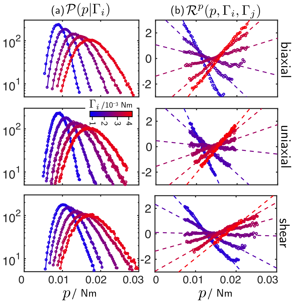
To proceed with the overlapping histogram methods, we utilize the ratio defined as $\mathcal{R}^{\sigma}(\sigma,\Gamma_{i},\Gamma_{j})=\log{\left[\mathcal{P}(\sigma|\Gamma_{i})/\mathcal{P}(\sigma|\Gamma_{j})\right]}$ for $\sigma\in\{p,\tau\}$. To give this ratio more meaning, consider the distribution of Eq. 1 under the assumption that the local force tiling area $a$ is strongly peaked at $\mathrm{det}(\hat{\sigma})$ [11, 9, 10]. In this limit, we can integrate Eq. 1 to isolate distributions:

for modified densities of state $\bar{\Omega}$ and $\tilde{\Omega}$ (see Supplemental Material for detailed integration). Thus, we have three temperature-like quantities: $\alpha^{p}$ and $\alpha^{\tau}$, the normal and deviatoric components of the angoricity tensor, and $\kappa$, the keramicity. By taking the logarithm ratios of these two distributions (Eq. 2-3) are

where $\mathcal{R}_{0}=\log{(Z_{i}/Z_{j})}$, and $(i,j)$ denotes two sets of states of pressure $\Gamma_{i}$ and $\Gamma_{j}$. Because ratios are sensitive to counting error in small values of the denominator, we only examine data for which $\mathcal{P}>10$.

In Fig. 2b and Fig. 3b, we illustrate typical logarithm ratios for several representative histograms; all ratios are computed relative to the same reference histogram. We observe that $\mathcal{R}^{p}$ is linear in $p$ with some arbitrary offset associated with the ratio of partition functions. The slope of $\mathcal{R}^{p}(p)$ gives the differential normal angoricity, $\alpha^{p}_{j}-\alpha^{p}_{i}$ between states at confining pressures $\Gamma_{j}$ and $\Gamma_{i}$. However, these ratios (Fig. 2b) can only be fit to reasonable precision to a first order polynomial in $p$, such that the difference $\kappa_{j}-\kappa_{i}$ cannot be established from this approach.

In contrast, similar ratios computed in Fig. 3b are found to be parabolic with a non-zero second-order coefficient, matching the expectation from Eq. 5, and we fit these ratios to a polynomial: $x\tau^{2}+y\tau+z$ The fit parameter $x$, corresponding to changes in the variance of force-moment component distributions, gives $x=\kappa_{i}-\kappa_{j}$, the difference in keramicity between states of global confining pressure $\Gamma_{i}$ and $\Gamma_{j}$. As before, we also identify the fit parameter $y$ to be associated with $y=\alpha^{\tau}_{j}-\alpha^{\tau}_{i}$. Thus, by taking the logarithm of the ratio of two closely-overlapped histograms with sufficient proximity in local free volume [6], we can compute relative measures of $\alpha^{p}$, $\alpha^{\tau}$, and $\kappa$ to within an additive constant $\mathcal{R}_{0}$ [7].

The presence of a $\tau^{2}$ term is found for all three protocols, in agreement with predictions by Wu and Teitel [11], in which the multipliers $\alpha^{p}$ and $\kappa$ are strictly related to only global measures of pressure. This allows the Boltzmann-like factor found in Eq. 1 to include terms that are quadratic in the components of the force-moment tensor.

As shown for angoricity under isotropic compression, we propose that the computed temperature-like state variables can be described by equations of state of the form $\alpha\Gamma=\lambda$ [39, 6, 7], where $\alpha$ represents any of $(\alpha^{p},\alpha^{\tau},\kappa)$ and $\lambda$ is a constant. To test experimental adherence to this hypothesis, we identify $\frac{1}{\alpha}=0$ (and $\frac{1}{\kappa}=0$) as corresponding to the jamming point ($\Gamma=0$) and reference differential temperature-like variable measurements accordingly (see Supplemental Material for procedure).

Repeating this procedure for all three temperature-like variables, we observe that the equation of state holds in all cases (Fig. 4). While for $\kappa$ the constant $\lambda$ is independent of loading protocol, for both $\alpha^{p}$ and $\alpha^{\tau}$ the constant exhibits significant protocol-dependence. Interestingly, $\lambda$ is always positive for $\alpha^{p}$, but the sign varies for $\alpha^{\tau}$ (values given in caption), corresponding to the direction of translation of $\mathcal{P}(\tau)$ in Fig. 3a, some of which are associated with experimental asymmetries. The magnitudes of the $\lambda$ agree within 2 standard errors for shear^A vs. shear^B, and the signs differ due to the change in sign of $\tau$. Because both components of $\hat{\alpha}$ are observed to be protocol-dependent, the tensoral angoricity is not valid as a variable of state, but rather a variable of process. By contrast, the keramicity behaves as a state variable.

Angoricity measures a granular packing’s ability to accommodate configurational rearrangements of equivalent global force-moment tensor (equivalently, stress) on a component-wise basis, $\alpha_{ij}=\partial S/\partial\Sigma_{ij}$. Thus, we have shown that as packings are loaded above jamming, they gain more and more configurations from the presence of forces to be distributed (Fig. 4a). Meanwhile, as $\frac{1}{\alpha^{p}}$ (Fig. 4a) and $\frac{1}{\alpha^{\tau}}$ (Fig. 4b) grow in magnitude, the responsiveness of the number of configurations to increases in global stress ($\partial S/\partial\Sigma$) decreases. Finally, the protocol by which a granular packing is loaded does not impact the trend that more compressed states gain fewer additional configurations from equivalent additions to the global Maxwell-Cremona area tiling (Fig. 4c).

We have demonstrated non-negligible curvature in the ratio of overlapped force-moment tensor histograms in jammed states of granular systems. This observation points towards a formulation of the force-moment ensemble that requires conservation of Maxwell-Cremona area tiling. The associated temperature-like variables all grow inversely with respect to confining pressure, but the keramicity, associated with the force tiling, is the only valid variable of state. The path-dependence of variables describing soft matter systems is not unfamiliar, but protocol-dependent scaling could be a route to a comprehensive granular equation of state. Meanwhile, the generalization of the force-moment ensemble to account for force-tiling statistics may yield a comprehensive statistical mechanics framework.

We are grateful for support from the National Science Foundation (DMR-1206808) and James S. McDonnell Foundation, and for useful conversations with Bob Behringer, Rafi Blumenfeld, Bulbul Chakraborty, Daphne Klotsa, James Puckett, Steve Teitel, and Brian Tighe.

References

- [1] S. F. Edwards and R. B. S. Oakeshott, Physica A 157, 1080 (1989).
- [2] H. M. Jaeger and S. R. Nagel, Science 255, 1523 (1992).
- [3] R. C. Ball and R. Blumenfeld, Physical Review Letters 88, 115505 (2002).
- [4] S. Martiniani, K. J. Schrenk, K. Ramola, B. Chakraborty, and D. Frenkel, Nature Physics (2017).
- [5] D. Bi, S. Henkes, K. E. Daniels, and B. Chakraborty, Annual Review of Condensed Matter Physics 6, 63 (2015).
- [6] S. Henkes, C. S. O’Hern, and B. Chakraborty, Physical Review Letters 99, 038002 (2007).
- [7] J. G. Puckett and K. E. Daniels, Physical Review Letters 110, 058001 (2013).
- [8] R. Blumenfeld and S. F. Edwards, Journal of Physical Chemistry B 113, 3981 (2009).
- [9] B. P. Tighe, A. R. T. van Eerd, and T. J. H. Vlugt, Physical Review Letters 100, 238001 (2008).
- [10] B. P. Tighe and T. J. H. Vlugt, Journal of Statistical Mechanics: Theory and Experiment 4, 04002 (2011).
- [11] Y. Wu and S. Teitel, Physical Review E 92, 022207 (2015).
- [12] S. Sarkar, D. Bi, J. Zhang, J. Ren, R. P. Behringer, and B. Chakraborty, Physical Review E 93, 042901 (2016).
- [13] T. S. Majmudar and R. P. Behringer, Nature 435 (2005).
- [14] T. Bertrand, R. P. Behringer, B. Chakraborty, C. S. O’Hern, and M. D. Shattuck, Physical Review E 93, 012901 (2016).
- [15] P. Chaudhuri, L. Berthier, and S. Sastry, Physical Review Letters 104, 165701 (2010).
- [16] J. D. Paulsen, N. C. Keim, and S. R. Nagel, Physical Review Letters 113, 068301 (2014).
- [17] C. Josserand, A. V. Tkachenko, D. M. Mueth, and H. M. Jaeger, Physical Review Letters 85, 3632 (2000).
- [18] S. M. Rubinstein, G. Cohen, and J. Fineberg, Physical Review Letters 96, 256103 (2006).
- [19] M. Huang and J. P. Sethna, Physical Review B 43, 3245 (1991).
- [20] D. Bi, J. Zhang, B. Chakraborty, and R. P. Behringer, Nature 480, 335 (2011).
- [21] H. A. Vinutha and S. Sastry, Nature Physics 12, 578 (2016).
- [22] A. J. Liu and S. R. Nagel, Annual Review of Condensed Matter Physics 1 (2010).
- [23] D. Bi, J. Zhang, R. P. Behringer, and B. Chakraborty, Europhysics Letters 102, 34002 (2013).
- [24] C. H. Rycroft, G. S. Grest, J. W. Landry, and M. Z. Bazant, Physical Review E 74, 021306 (2006).
- [25] K. E. Daniels, J. E. Kollmer, and J. G. Puckett, Review of Scientific Instruments 88, 051808 (2017).
- [26] J. E. Kollmer, Photo-Elastic Grain Solver, http://github.com/jekollmer/PEGS.
- [27] Link to data at http://DataDryad.org will go here.
- [28] C. Song, P. Wang, and H. A. Makse, Nature 453, 629 (2008).
- [29] T. Aste and T. Di Matteo, Physical Review E 77, 021309 (2008).
- [30] S. McNamara, P. Richard, S. K. de Richter, G. Le Caër, and R. Delannay, Physical Review E 80, 031301 (2009).
- [31] F. Lechenault, F. da Cruz, O. Dauchot, and E. Bertin, Journal of Statistical Mechanics: Theory and Experiment 2006, 07009 (2006).
- [32] J. Ren, J. A. Dijksman, and R. P. Behringer, Physical Review Letters 110, 018302 (2013).
- [33] B. Andreotti, Y. Forterre, and O. Pouliquen, Granular media: between fluid and solid (Cambridge University Press, 2013).
- [34] B. P. Tighe, Granular Matter 16 (2014).
- [35] H. Hotelling, Analysis of a Complex of Statistical Variables into Principal Components (Warwick & York, 1933).
- [36] P. Labastie and R. L. Whetten, Physical Review Letters 65, 1567 (1990).
- [37] D. S. Dean and A. Lefèvre, Physical Review Letters 90, 198301 (2003).
- [38] T. B. Nguyen and A. Amon, Europhysics Letters 116, 28007 (2016).
- [39] S. Henkes and B. Chakraborty, Physical Review Letters 95, 198002 (2005).
Supplemental Material