OGLE-2016-BLG-1266: A Probable Brown-Dwarf/Planet Binary at the Deuterium Fusion Limit
Abstract
We report the discovery, via the microlensing method, of a new very-low-mass binary system. By combining measurements from Earth and from the Spitzer telescope in Earth-trailing orbit, we are able to measure the microlensing parallax of the event, and find that the lens likely consists of an + super-Jupiter / brown-dwarf pair. The binary is located at a distance of kpc in the Galactic Plane, and the components have a projected separation of AU.
Two alternative solutions with much lower likelihoods are also discussed, an 8- and 6- model and a 90- and 70- model. Although disfavored at the 3- and 5- levels, these alternatives cannot be rejected entirely. We show how the more-massive of these models could be tested with future direct imaging.
I Introduction
The growing number of detections of super-Jupiter-mass objects, both isolated and in orbit around objects of higher mass, raises challenges of interpretation and classification.
Formal definitions of what constitutes a “planet” tend to be based on the mass or interior physics of the object. The IAU Working Group on Extrasolar Planets (which existed until 2006) considered the deuterium fusion limit ( for solar metallicity) to be the dividing line between planets and brown dwarfs for objects that orbit stars. They also considered substellar objects with masses above the deuterium fusion limit to always be brown dwarfs. The NASA Exoplanet Archive adopts a looser definition for inclusion in their planet tables, namely that the inclusion of an object as a planet is made provided that its mass is less that 30 and it is associated with a host star11 1 Confusingly, the Archive violates its own policy by including objects with brown-dwarf hosts. https://exoplanetarchive.ipac.caltech.edu/docs/exoplanet_criteria.html.
On the other hand, the logical definition for what constitutes a “planet” would be based on formation mechanism, i.e., whether the object formed in a disk or through direct collapse of the gas cloud. This might suggest a distinction between super-Jupiter-mass objects that orbit stars and those that orbit hosts of comparable mass (i.e., very low mass, brown dwarf-brown dwarf binaries), and raises questions about how to classify those without hosts. In fact, the observational community tends to make a distinction between super-Jupiters orbiting stars and those orbiting brown dwarfs. Best et al. [10] refer to 2MASS J11193254-1137466 (a member of the TW Hydrae Association) as a pair of 3.7 brown dwarfs, and suggest that the system is a product of normal star formation processes. In contrast, Lovis & Mayor [45] refer to the 10.6 object orbiting the 2.4 star TYC 5409-2156-1 as a planet, and argue that an abrupt transition between planets and brown dwarfs has little meaning if both categories of objects are formed by the same physical process. Likewise Carson et al. [18] argue that a planetary classification rather than brown dwarf is appropriate for a 12.8 body orbiting the 2.5 host star, And.
Formal definitions do not capture these nuances. The IAU makes a specific distinction for isolated objects located in young star clusters: below the deuterium-burning limit, they are classified as “sub-brown dwarfs” [12]. However, the classification of an object at or below the deuterium fusion limit that is gravitationally bound to another sub-stellar object is not currently defined by the IAU. Neither is the case of an isolated object of that mass located outside a young cluster.
Precise definitions are complicated by the fact that without observing the actual formation of the objects, it is impossible to say what mechanism led to their formation and where the boundary should be. For example, Mordasini et al. [48] show that it is theoretically feasible to grow super-Jupiters by core accretion in a proto-planetary disk up to at least . At the same time, Schlaufman [59] has recently suggested that any companions to solar-type stars with mass should not be considered planets, i.e., could not have formed by core accretion. However, since the Schlaufman study was based solely on transiting (i.e., short period) objects, it is unclear whether or not this result truly reflects something about formation rather than the subsequent migration of the objects. Defining the boundary between “planets” and “brown dwarf companions” is further complicated by the question of whether or not gravitational instability of a disk should be considered to form planets or brown dwarfs. Certainly, though, the choice of the deuterium fusion limit as the planet / brown-dwarf boundary is arbitrary and confusing [4].
It is unclear at this time whether brown-dwarf/super-Jupiter binaries belong to the population of objects that formed like binary stars from the collapse of molecular clouds, or if some other mechanism, such as ejection from a higher-multiplicity system is responsible. Hydrodynamic simulations of the collapse of a large star-forming molecular cloud by Bate [5] resulted in 450 stars and 800 brown dwarfs. Of these, some brown dwarfs with masses below were formed but no binaries with primary masses below .
Understanding the differences in super-Jupiter-mass objects as a function of their host mass requires the discovery of more such objects, especially those with very-low-mass (brown dwarf) hosts. In addition to the Best et al. [10] binary, a handful of very-low-mass binaries have been detected by photometric methods in young open clusters and star forming regions [46]. However, mass estimates for these objects rely on theoretical models of their evolution. The uncertainties are large, and the results are strongly dependent on the assumed age of the systems.
Microlensing offers an entirely different avenue for probing the population of very-low-mass binaries. In recent years three very-low mass binaries have been detected through the channel of gravitational microlensing [20, 37]. In contrast to the photometric detections, microlensing binaries can have direct and reliable mass estimates, independent of brown-dwarf evolutionary theory. Furthermore, these objects are located at large distances in the Galactic Disk and are outside of young, star-forming clusters.
In this paper we report the detection of a fourth very-low mass binary system by microlensing. This new system is composed of a 15.7- brown dwarf plus a companion just below the deuterium fusion limit.
II Gravitational Microlensing
Gravitational microlensing is an effect for which the brightness of a distant star (the source) is magnified due to the bending of light by the gravity of a nearer object (the lens). Typically, microlensing events are detected each year in the direction of the Galactic Bulge by the OGLE22 2 http://ogle.astrouw.edu.pl/ogle4/ews/ews.html, MOA33 3 https://www.massey.ac.nz/iabond/moa/alerts/ and KMTNet44 4 http://kmtnet.kasi.re.kr/kmtnet-eng/ surveys.
The characteristic angular scale for microlensing is the Einstein radius,
| (1) |
where is the total mass of the lens system, , are the distances from Earth to the lens and source, is the lens-source relative parallax, and .
The magnification, , of a standard binary microlensing event can be described by seven parameters in the lens frame. These represent the angular separation of the lens components (), their mass ratio (), the angular source radius in units of (), the angle of the source trajectory from the lens axis (), the angular distance of closest approach of the source to the lens center of mass in units of (), the time of closest approach () and the Einstein radius crossing time (). Two additional linear parameters, the source and blend flux and , are required for each data set to map the magnification onto the observed flux , i.e.,
| (2) |
If the source angular radius, , can be measured independently (usually from its color and an assumption that it lies behind the same column of dust as the Galactic Bulge), then the angular Einstein radius can be determined.
Additionally, if the microlensing event can be viewed by two observers with a significant spatial separation (say from Earth and a distant Solar-orbiting satellite; Refsdal 56) or if the event timescale is long enough that Earth moves appreciably in its orbit, then the microlensing parallax vector [31, 14] may be measured. Then , and hence can be determined.
III Observations
The event OGLE-2016-BLG-1266 (17:51:24.86, -29:44:32.1) J2000.0, galactic coordinates , was alerted by the Optical Gravitational Lensing Experiment [63, OGLE] on 2016 July 4 UT 11:24, based on observations from the 1.3-m Warsaw Telescope at the Las Campanas Observatory, Chile. The OGLE observations were taken at a cadence of 55 minutes. Photometry of the OGLE images was extracted using the standard OGLE difference-imaging pipeline.
OGLE-2016-BLG-1266 was also observed by the Korea Microlensing Telescope Network [43, KMTNet] using identical telescopes at the Cerro Tololo Inter-American Observatory in Chile; the South African Astronomical Observatory at Sutherland, South Africa; and the Siding Spring Observatory, Australia. It was identified as SAO42T0504.003968 [41, 42]. Both the OGLE and KMTNet observations were taken as part of regular surveys, with cadence uninformed by the detection of the event. For KMTNet, the event is located in two overlapping survey fields, BLG02 and BLG42, giving an effective cadence of 15 minutes. The primary KMTNet observations were taken in the band, supplemented by an occasional -band observation.
Photometry was extracted from the KMTNet observations using the software package PYDIA [2], which employs a difference-imaging algorithm based on the modified-delta-basis-function approach of Bramich et al. [13]. The data from field BLG02 observed from SAAO were discarded as they were affected by a cosmetic feature of the detector. The remaining KMTNet lightcurves were filtered using various image quality criteria and without reference to the lightcurve.
The event was also observed by the Spitzer space telescope at a wavelength of 3.6 m using the IRAC instrument [24]. These observations were acquired as part of a multi-year project to measure the distances of microlensing planets in the Galaxy [15, 65]. OGLE-2016-BLG-1266 was announced as a Spitzer target at 2016 July 10 UT 21:15, based on the possibility that it would rise to high magnification, and uploaded to Spitzer the next day. The first observation was at UT 18:18 on 16 July. In total, 6 observations were taken during the following 7 days. The sequence of observations was terminated at that point due to Spitzer’s Sun-angle restriction. The event was observed for a further 9 epochs by Spitzer in 2017 after the magnification had fallen to baseline levels. Spitzer photometry was extracted using the methods described in Calchi Novati et al. [16].
IV Microlensing model from Earth-based observations
The combined ground-based lightcurve of OGLE-2016-BLG-1266 is shown in Figure 1. It displays a smooth double peak, suggestive of a resolved source crossing a pair of caustics, generated by a binary lens.
Our analysis of the lightcurve was undertaken using a modified version of the GPU-accelerated code of McDougall & Albrow [47]. Initially we performed a search over a fixed grid of , where is the distance from the centers of caustics (a reparameterisation of ). This established a number of possible approximate solutions that were used as starting points for Markov Chain Monte Carlo minimization using the EMCEE ensemble sampler [25]. The magnification calculations used the image-centered inverse ray shooting method [7, 6] for locations within three source radii of a caustic, the hexadecapole approximation [54, 32] for distances between 3 and 30 source radii, and the point-source binary-lens approximation otherwise. For the ray shooting calculations, we used a fixed source limb-darkening coefficient, , appropriate for the source star color that we derive in the following section. From these Markov Chains, a single viable solution was identified at , corresponding to the source passing over one of the two triangular caustics produced by a close binary. The corresponding lightcurve and caustic geometry are shown in Figure 1. In this paper we plot lightcurves on a scale of , where , and and are model-dependent. We note that the model implies a small negative blending for the OGLE data (), equivalent to the flux of an star. As discussed by Park et al. [52], such low-level negative blending is a normal feature of microlensing photometry in very crowded bulge fields.
V Source star radius
Using KMTNet CTIO BLG42 images in the and bands, we have constructed a DoPHOT [58] instrumental color-magnitude diagram (CMD) for stars in a 3 arcmin 3 arcmin box centered on the event (left panel of Figure 2). From this diagram we measure the red clump centroid to be at . From regression of -band flux against -band flux during the event, checked by a two-parameter fit of the -band-determined magnification profile to the -band data, we determine a deblended instrumental source color and thus an offset from the clump .
We have also constructed an instrumental CMD from -band images acquired with the ANDICAM instrument at the 1.3-m CTIO telescope, and -band catalog measurements of the field from the VVV survey [57] (right panel of Figure 2). Although -band images were acquired at CTIO simultaneously with the -band images, we opt to use VVV measurements for the CMD as they are deeper. We measure the red clump in this CMD at . From regression of ANDICAM and measurements of the microlensing event, we determine , which when adjusted for an offset (determined by regression of field stars) implies an instrumental source color and an offset from the red clump .
In principle, color offsets from the Red Clump are filter dependent. However, since our measurement of is essentially zero, it implies an offset from the clump of zero in any filters. Thus we count this measurement as implying , and average it with our previous measurement, , to obtain a final offset of .
OGLE-2016-BLG-1266 has a galactic longitude close to , so from Nataf et al. [51] and Bensby et al. [8] we adopt an intrinsic clump centroid . From the offset of the deblended source color from the red clump center on the instrumental CMDs, we calculate the intrinsic source color . Additionally, from the parameter determined from the lightcurve model, we find on the KMT BLG42 instrumental system, and .
To determine the angular source size, we convert to using the empirical color-color equations of Bessell & Brett [9]. Then, from Kervella et al. [40], we find a source angular radius as.
For the same field of stars, using the methods described in Shvartzvald et al. [62] and Calchi Novati et al. [16], we determine that on a Spitzer system with a 25th magnitude zero point.
From the source angular radius and the lightcurve model we can compute . The geocentric lens-source relative proper motion is then .
Comparing and with samples from the Han & Gould [36] model of the Galactic Bulge and Disk, Figure 7 in Penny et al. [55], (and at this stage ignoring any difference between and ) we note that is at the extreme of what is possible for a Bulge lens, so the lens is likely in the Galactic Disk. (See also Figure 1 in Han & Chang [35]). Our measurement of implies a total lens mass of 10 if the lens distance is 1.3 kpc and 100 if the distance is 5.1 kpc.
VI Parallax Constraints
The orbit of Earth around the Sun introduces a parallax effect on ground-based observations of microlensing events [28, 30]. Although present for all such observations, it is usually only detectable for events with a timescale d. The effect manifests as a sinusoidal perturbation on an otherwise-linear projected source trajectory in the lens plane (see for example Han et al. [38], Han et al. [37], Park et al. [53], Furusawa et al. [26]).
In addition to this annual parallax effect, we fit for the satellite parallax effect. The Spitzer telescope is in an Earth-trailing solar orbit, behind Earth in 2016. At the time of peak magnification, Spitzer was located at coordinates (RA,DEC) = (10:25,09:08) and a distance of 1.484 AU from Earth. Perpendicular to the direction of OGLE-2016-BLG-1266, the projected distance of Spitzer from Earth was AU. When viewed from Spitzer, the source trajectory across the lens plane is offset by a vector , in directions (perpendicular, parallel) to the trajectory observed from Earth. The parallel offset is simply,
| (3) |
but the perpendicular offset suffers from a four-fold satellite parallax degeneracy due to the symmetry of the magnification field about the lens axis,
| (4) |
as illustrated in Gould [29]. The sign convention we adopt here is that a positive value of indicates that, during its projected trajectory, the source approaches the lens on its right hand side.
We make an initial fit to the Spitzer lightcurve by adopting the ground-based model parameters and exploring a grid in to offset from . These constant offset values are used as the reference indices for the grid, but the calculations of the actual model Spitzer lightcurve use the true offset of each data point at its epoch of observation.
At each point in the grid we map the magnification to the observed Spitzer flux using Equation (2).
To include the Spitzer source flux constraint derived in the previous section, we penalise with an additional term,
| (5) |
where is the -band to -band flux ratio and is the uncertainty in [60]. Mathematically, this is entirely equivalent to a prior on the probability of the model parameters that generate . We elected not to use the Shin et al. [60] method of adding an additional penalty for deviations greater than 2-.
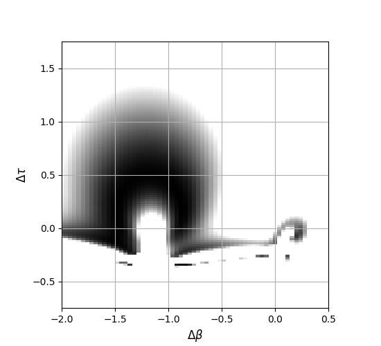
The grids in for the unconstrained and source-flux-constrained cases are shown in Figure 3. Comparing the constrained with the unconstrained solutions, it is clear that there is a broad region in space that is consistent with both the source-flux-constrained and unconstrained models for the Spitzer data.
In the unconstrained case, the lowest- solution corresponds to a small region at , which is not visible in the corresponding flux-constrained map. It is instructive to consider the penalty that the source flux constraint imposes for this particular . The -band to -band source-flux ratio constraint is from our CMD analysis. The unconstrained model at that point has . It is very unlikely that our -band flux measurement is in error by a factor of 8 (i.e., more than 2 magnitudes). Thus we consider that this “best” of the unconstrained models is ruled out by the -band measurement, and we only consider the constrained models from here on.
To explore the identified solution space, we have run full EMCEE Markov Chains incorporating the standard binary microlensing model with two parallax parameters for the combined ground-based and Spitzer data, incorporating the Spitzer source flux constraint. Chains seeded from various points in space all converged to one of the two points indicated with plus signs in Figure 3.
Solution A (“green plus”) corresponds to trajectories for which the six 2016 Spitzer data points are located to the left of the central caustic in Figure 1, interior to (i.e., closer to the lens axis than) the Earth-viewed trajectory. In this region, the magnification is declining smoothly with a steeper slope than the ground-based model. The minimum is located in this solution region at .
Solution B (“yellow plus”) is located slightly exterior to the Earth-viewed trajectory. The lightcurve corresponding to this Spitzer-viewed trajectory incorporates a small peak close to the first data point due to a high magnification region in an extension of a cusp from the planetary caustic. The minimum for this solution is located at , and is disfavored relative to Solution A by .
The microlensing parallax, , depends on as
| (6) |
where is the distance of Spitzer from Earth, perpendicular to the line of sight to the lens. At the peak of the event, , so that Solution A (“green plus”) has , while Solution B (“yellow plus”) has .
VII Satellite degeneracy
As discussed at the beginning of the previous section, there exists a four-fold degeneracy in (Equation ( 4)). To further investigate the satellite degeneracy, we adopted the A (green) and B (yellow) source-flux-constrained solutions from Figure 3 and ran EMCEE chains to explore the complete set of solution regions.
For Solution A at (green plus symbol in the right panel of Figure 3), the and trajectories lie along the lens axis and are almost identical for . We refer to these as the A (“green”) solutions.
In contrast, for Solution B (yellow plus symbol in the right panel of figure Figure 3) at , there is a separate trajectory that lies above the upper triangular caustic (and was outside the range of the grid search). We refer to these solutions as the B (“yellow”) solutions.
Microlensing parameters derived from the eight models are shown in the left columns for each geometry in Tables 1 and 2. Given the apparent degeneracies, the eight solutions correspond to three different microlensing parallaxes; small-parallax B (), large-parallax B (), and A (). Representative lightcurves for the A (green) and B (yellow) geometries are shown in Figure 4.
For the solution-A trajectories, there is a small difference in the solutions due to the small annual-parallax-induced curvature in each trajectory, with the solution being marginally favored. The solutions for each are fully degenerate.
In contrast, the second set of models (solution B) separate in for the two cases that has the same or opposite sign as (with the opposite sign models favored by ), but are otherwise degenerate in .
VIII Lens orbital motion
Ignoring projection effects, a Keplerian orbit for the masses and separation derived in the previous section would have a period of about 1.6 years. This suggests that lens orbital motion may be a detectable and significant effect. We have thus extended our models with first order lens motion parameters and .
We require that the complete set of model parameters are consistent with a bound orbit, in particular that the projected kinetic energy be less than the potential energy. From Dong et al. [22]
| (7) |
In convenient units, this leads to a constraint,
| (8) |
From Section V, we assume that the source is at the red-clump distance, 8.18 kpc, and that . We implement the constraint as a prior, with the hard upper boundary softened by the uncertainty in .
We have run models seeded from the eight satellite-parallax degenerate solution regions discussed above. The resulting parameters are listed in the right hand columns for each geometry in Tables 1 and 2, and the geometries are displayed in Figure 5.
Chains for solution A (green) converge to almost the same solution, again with a small difference of 4 between the solutions. The overall is lowered by 12 relative to the models without lens orbital motion.
Again, as expected, the solution-B models (yellow) converge to different solutions for . The and solutions have smaller than the and solutions. Relative to the solution-A model, the best of these is disfavored by .
In Figure 6 we show the posterior parameter distribution for the solution A model (which ultimately becomes out favored model in Section 8 below). Corresponding plots for the other 7 models are similar. The effect of the kinetic energy prior is apparent in and . If it were not for this physical constraint, the data would force to . The kinetic energy prior has an effect in all cases, but each energy-constrained solution is always part of the same minimum as a corresponding unrestricted (non-physical) model.
Overall, the inclusion of lens orbital motion in the models changes slightly the other parameters, and improves slightly for all models.
Both of the A solutions imply that the lens is a binary with component masses of 16 and 12 Jupiter masses. The higher mass component is a brown dwarf, and the lower mass component is on the dividing line between a brown dwarf and a super-Jupiter planet (sub-brown dwarf). The lens is located at a distance of 3.0 kpc from Earth, and the components have a projected separation of 0.4 AU.
The “same-sign” B solutions (with relative to the A solutions) are for a 90 and 68 Jupiter-mass binary at 6.2 kpc with a projected separation of 0.9 AU, while the “opposite-sign” B solutions (with relative to the A solutions) are for an 8 and 6 Jupiter-mass binary at 2.1 kpc with a projected separation of 0.3 AU.
IX Which solution is correct?
In this section we use several lines of evidence to assess the solutions obtained above. Our approach is similar to that of Calchi Novati [17].
IX.1 The best lightcurve fit
In Tables 1 and 2 we list for each fit. In all cases, we have found that the six Spitzer data points from 2016 comprise the major source of . Irrespective of whether lens orbital motion is included in the models, the A (green) series of solutions have the best formal fit, with the models being slightly better than the models. The B (yellow) series of solutions are less favored, but not by a large amount. Formally, the probability of each solution relative to the best one is lowered by , so that the best of the large-parallax B solutions has a probability of only 0.040 relative to the A solution (i.e., a 2.5- difference), and the best small-parallax B solution has a relative probability of (4.4-). However, these formal probabilities rest on the assumption that all data are independent and Gaussian-distributed, and that data uncertainties are accurate. Such conditions are never satisfied for microlensing photometry. On this basis, we are unable to reject entirely the yellow solutions.
IX.2 The Rich argument
The “Rich argument” is elucidated in Calchi Novati et al. [15]. Briefly, for a point-lens microlensing event, when considering two alternate satellite-degenerate solutions from the same model, the one with the smallest parallax is usually correct. This is because if the true parallax solution is small, it will always generate a large-parallax counterpart. However, if the true parallax is large, then there is a much smaller probability, , that the parallax of the counterpart solution is small. This probability factor is based on the rotational symmetry of the magnification field about the lens. For incomplete satellite lightcurves, the true probability factor can be larger because a two-parameter fit can map different magnification patterns to the same flux lightcurve.
For binary lenses, the geometric degeneracy on which the Rich argument is based, exists only for cases in which the source trajectory is almost parallel to the lens axis, as is the situation we are considering here. The two B (yellow) solutions represent an analogous situation to the large- and small-parallax solutions for a point lens. However, we cannot naively apply the point-lens relative probability factor because the magnification pattern for a binary lens does not have the rotational symmetry of the single-lens pattern, and our Spitzer lightcurve does not have full coverage.
The A-solution degeneracy with either of the B solutions is not a true geometric degeneracy. It exists because of our limited epochs of Spitzer observations and would not be present if we had full temporal coverage.
We have assessed the relative probabilities of the various solutions by simulating Spitzer lightcurves for the three different parallax amplitudes () and for different angles () with respect to the source trajectory. For each simulation, we held the ground-determined microlensing parameters constant, and computed a flux lightcurve by combining the previously-determined Spitzer source and blend flux with the the magnification, at the Spitzer epochs. We then added the residuals of the Spitzer data relative to the A model fit.
To determine the probability factor for the large-parallax B solution relative to the small-parallax B solution, we have simulated lightcurves for 360 values of for the B parallax amplitude. For each of these we have made a two-parameter, source-flux constrained fit using the magnification at the constant B parallax amplitude, found from the transformation , and allowing the angle to vary. For each , we accumulate the between the large-parallax and small-parallax fits. We then compute the probability that a true small parallax would have a large parallax degeneracy as being the fraction of angles for which is less than some threshold value. We then repeat this exercise in reverse, generating a set of large-parallax simulations, and finding the small-parallax fits. The ratio of these two probabilities then gives the a-priori probability of a large parallax solution relative to a small one for the given geometry, satellite observation epochs, source-flux constraints, and observation residuals, independent of the actual measured satellite flux values. To simplify the interpretation, we have made these synthetic lightcurves and fits without including the effects of lens orbital motion.
We adopt a threshold similar to the range of actual measured for our different degenerate solutions discussed in the previous sections. We find that there is a 0.43 probability that a true small B parallax would generate a large B parallax degenerate solution. If the source trajectory were exactly parallel to the lens axis, we would expect this factor to be exactly 1.0. (In the current geometry, the factor rises to unity were we to increase our threshold to 80.) We find that there is a 0.40 probability that a true large B parallax can generate a small B parallax degenerate solution. This probability is much larger than what would be the case for continuous Spitzer lightcurve coverage. Combined, we find an overall probability of 0.935 of a large B parallax relative to a small B parallax.
To determine the probability factor for the A model relative to the small-parallax B model we carry out a similar calculation, but use the A model parallax amplitude rather than the parallax of the alt solution. From these calculations we find that there is a 0.33 probability that a true small B parallax would generate a degenerate solution with the parallax amplitude of the A model, a 0.37 probability that a true solution with the parallax amplitude of the A model would generate a degenerate small-parallax B solution, and an overall probability of 1.11 of an A-model parallax relative to a small-parallax B model.
In summary, we have found that the overall a-priori relative probability factors stemming from this specific geometry and set of Spitzer observation epochs are close to unity, so have little effect on our relative assessment of the different solutions.
IX.3 Galactic rotation
For a flat rotation curve, and from the Local Standard of Rest (LSR) perspective, the rotational component of the proper motion of a disk star interior to the Sun’s orbit and relative to the Bulge, , is independent of the star’s distance. Projected onto the lens plane, the disk of the Milky Way rotates in a direction North of East. In the absence of random velocity dispersions for the disk and Bulge, we would expect disk lenses to have a relative proper motion in this direction if we were observing from the LSR. Adopting , and a Bulge distance of 8.18 kpc, gives . Added to this overall disk rotation, individual disk stars have a velocity dispersion, . Given its low galactic latitude, the lens in OGLE-2016-BLG-1266 is almost certainly part of the old thin disk, for which .
From its location on the CMD, we assume our source star is part of the Bulge population. We have adopted , as an average of the Y and Z direction Bulge velocity dispersions from Bland-Hawthorn & Gerhard [11]. To compare the relative lens-source proper motion for our various models with that expected for disk lenses, we transform to the LSR by adding the projection of Sun’s peculiar velocity, , to the relative lens-source proper motion. The resultant LSR relative lens-source proper motions, for each model, are shown in Figure 7 along with the galactic expectation, with a dispersion .
We can see that the A (green) solutions for are well aligned with Galactic Disk rotation. The B (yellow) solutions for are also plausible, but the remaining models are rather improbable.
For each model solution, we can form a probability that the lens has the expected proper motion of the Galactic Disk,
| (9) |
(see Tables 1 and 2). Based on their proper motion correspondence with our galactic rotation model, the B (yellow) models are 4 - 15 times less probable than the A (green) models.
IX.4 Combined probability
We have discussed three factors that we consider important for assessing the relative merits of the A and B series of models for OGLE-2016-BLG-1266. For each of these, we can assign a relative probability; from the lightcurve fits, from the Rich argument, and from the proper motion correspondence to galactic rotation. We have multiplied the three probabilities for each model and normalised to the maximum to compute a net relative probability, , also listed in Tables 1 and 2.
Considering all factors, the most-favored solutions are the degenerate A-series models. These models imply a 16- + 12- mass lens at a distance of 3.1 kpc. We note that these solutions have a significantly larger parallax ( than any of the previous events measured by Spitzer. (The next largest parallax is OGLE-2016-BLG-1195 with ; Shvartzvald et al. 62.)
Relative to the A solutions, the best of the B solutions is the large-parallax model with a relative probability of . The small-parallax model has a relative probability of . Respectively, these models imply an 8- + 6- mass lens at a distance of 2.0 kpc and a 90- + 70- pair at 6.2 kpc. The relative probabilities correspond to 2.91- and 4.86- differences from the favored model.
IX.5 Is the favored lens mass plausible?
The initial mass function (IMF) for brown dwarfs below = 0.1 M☉ () is not well established, and may depend on environment. The Kroupa [44] and Chabrier [19] IMFs for single objects increases toward lower mass in this range, but there is evidence that the MF “turns over” at increasingly higher masses with age in stellar clusters [19]. There is little evidence of a large decline between 0.1 M☉ and 0.01 M☉ in the studies of Alves de Oliveira et al. [3], Jeffries [39], Gagné et al. [27]. Overall, there is little reason from the lens-mass results to reject the high-parallax low-mass model in favor of the lower-parallax higher-mass one.
IX.6 Falsification of the favored model
Our adopted model for OGLE-2016-BLG-1266 is for a 16- + 12- mass lens at a distance of 3.1 kpc. Given its low mass, we do not expect the lens to be directly observable with any presently conceived instruments. This is also the case for the B model, which corresponds to a binary composed of two planetary-mass objects.
However, the more massive of the plausible challenger models (B ) consists of a 90- + 70- mass lens at a distance of 6.2 kpc. From Dupuy & Liu [23],we expect that this pair would have absolute and magnitudes of 11 and 10, and so apparent magnitudes , . This solution has a heliocentric lens-source relative proper motion of mas yr-1. In ten years there would be a separation of 92 mas between the lens and the source in the indicated direction. Resolving the lens and source for the high-mass model should be within the first-light capability of diffraction-limited near-infrared imagers on the coming generation of extremely large telescopes, for example ELT-CAM on E-ELT.
X Discussion
Objects like OGLE-2016-BLG-1266 challenge our understanding of what is meant by a planet. If the low-mass component of our favored model were associated with a star, or a brown dwarf with significantly higher mass, then it would be be described as a planet. However, with masses so close, both components of the binary may instead belong to the very low-mass end of the stellar initial mass function. We note that the survey of Mróz et al. [49] has identified several short-time-scale binary events that may be part of such a population.
For several reasons, detecting single planetary mass objects (often referred to as “free-floating planets”) by the microlensing method is a more difficult task than detecting binary lenses. Firstly, the peak magnification is generally lower and thus will have a lower probability of detection as a microlensing event. Second, the mass of single lenses can only be inferred from a measurement of , and that parameter is extremely degenerate with blending, and subject to incorrect inference if derived from lightcurve data with any systematic correlation between neighboring points. Third, it is difficult to establish a microlensing parallax measurement for short- events, because for Earth-orbital parallax measurements the trajectory of Earth does not deviate much from linear during the event duration, and for satellite parallaxes it is difficult to target satellite observations while the event is still significantly magnified.
There are currently four published single-lens events with secure lens-mass measurements from Spitzer [66, 21, 61], and two from ground-only measurements [34, 64], all with masses in the brown-dwarf regime.
There are currently no secure detections of single planetary mass objects by the microlensing method [49]. The object very recently detected by Mroz et al. [50] may be the first isolated “planet”, but even for that event, the presence of a stellar host at a separation AU cannot be ruled out.
Single planetary-mass lenses may be found more readily in the future with the advent of the WFIRST mission, which will observe Galactic Bulge microlensing events with high photometric precision and less blending than from the ground. Gould [33] shows how the presence of stellar companions to such single-lens candidates can be detected or ruled out by WFIRST and ground-based adaptive-optics observations. We should always bear in mind that, in the absence of an evolutionary history, the designation of low-mass single lenses as free-floating “planets” may be incorrect.
XI Summary
Using data from the KMTNet and OGLE telescopes, and the Spitzer satellite, we have analysed the microlensing event OGLE-2016-BLG-1266. Our models show that the lens is very likely composed of a 16- + 12- binary at a distance of 3.1 kpc.
Two alternative models are unlikely, but cannot be entirely rejected. One of these models corresponds to a 6- + 8- “planet-planet” binary at a distance of 2.0 kpc. The second of these alternatives, a 70- + 90- binary at 6.2 kpc, would be directly observable with the next generation of telescopes and instrumentation.
XII Acknowledgements
MDA is supported by the Marsden Fund under contract UOC1602, and is grateful for the award of an ESO Visiting Fellowship in December 2017 / January 2018 during which time this paper was completed. Work by WZ, YKJ, and AG were supported by AST-1516842 from the US NSF. WZ, IGS, and AG were supported by JPL grant 1500811. Work by C.H. was supported by the grant (2017R1A4A1015178) of National Research Foundation of Korea. This research has made use of the KMTNet system operated by the Korea Astronomy and Space Science Institute (KASI) and the data were obtained at three host sites of CTIO in Chile, SAAO in South Africa, and SSO in Australia. The OGLE project has received funding from the National Science Centre, Poland, grant MAESTRO 2014/14/A/ST9/00121 to AU. Work by YS was supported by an appointment to the NASA Postdoctoral Program at the Jet Propulsion Laboratory, California Institute of Technology, administered by Universities Space Research Association through a contract with NASA. This work is based in part on observations made with the Spitzer Space Telescope, which is operated by the Jet Propulsion Laboratory, California Institute of Technology under a contract with NASA.
References
- [2] Albrow, M. 2017, MichaelDAlbrow/pyDIA: Initial release on github., , , doi:10.5281/zenodo.268049. https://doi.org/10.5281/zenodo.268049
- [3] Alves de Oliveira, C., Moraux, E., Bouvier, J., et al. 2013, A&A, 549, A123
- [4] Baraffe, I., Chabrier, G., & Barman, T. 2008, A&A, 482, 315
- [5] Bate, M. R. 2012, MNRAS, 419, 3115
- [6] Bennett, D. P. 2010, ApJ, 716, 1408
- [7] Bennett, D. P., & Rhie, S. H. 1996, ApJ, 472, 660
- [8] Bensby, T., Yee, J. C., Feltzing, S., et al. 2013, A&A, 549, A147
- [9] Bessell, M. S., & Brett, J. M. 1988, PASP, 100, 1134
- [10] Best, W. M. J., Liu, M. C., Dupuy, T. J., & Magnier, E. A. 2017, The Astrophysical Journal Letters, 843, L4. http://stacks.iop.org/2041-8205/843/i=1/a=L4
- [11] Bland-Hawthorn, J., & Gerhard, O. 2016, ARA&A, 54, 529
- [12] Boss, A. P., Butler, R. P., Hubbard, W. B., et al. 2007, Transactions of the International Astronomical Union, Series A, 26, 183
- [13] Bramich, D. M., Horne, K., Albrow, M. D., et al. 2013, MNRAS, 428, 2275
- [14] Calchi Novati, S., & Scarpetta, G. 2016, ApJ, 824, 109
- [15] Calchi Novati, S., Gould, A., Udalski, A., et al. 2015a, ApJ, 804, 20
- [16] Calchi Novati, S., Gould, A., Yee, J. C., et al. 2015b, ApJ, 814, 92
- [17] Calchi Novati, S. e. a. 2018, AAS, submitted
- [18] Carson, J., Thalmann, C., Janson, M., et al. 2013, ApJ, 763, L32
- [19] Chabrier, G. 2003, PASP, 115, 763
- [20] Choi, J.-Y., Han, C., Udalski, A., et al. 2013, ApJ, 768, 129
- [21] Chung, S.-J., Zhu, W., Udalski, A., et al. 2017, ApJ, 838, 154
- [22] Dong, S., Gould, A., Udalski, A., et al. 2009, ApJ, 695, 970
- [23] Dupuy, T. J., & Liu, M. C. 2017, ApJS, 231, 15
- [24] Fazio, G. G., Hora, J. L., Allen, L. E., et al. 2004, ApJS, 154, 10
- [25] Foreman-Mackey, D., Hogg, D. W., Lang, D., & Goodman, J. 2013, PASP, 125, 306
- [26] Furusawa, K., Udalski, A., Sumi, T., et al. 2013, ApJ, 779, 91
- [27] Gagné, J., Faherty, J. K., Mamajek, E. E., et al. 2017, ApJS, 228, 18
- [28] Gould, A. 1992, ApJ, 392, 442
- [29] —. 1994, ApJ, 421, L75
- [30] —. 2000, ApJ, 542, 785
- [31] —. 2004, ApJ, 606, 319
- [32] —. 2008, ApJ, 681, 1593
- [33] —. 2016, Journal of Korean Astronomical Society, 49, 123
- [34] Gould, A., Udalski, A., Monard, B., et al. 2009, ApJ, 698, L147
- [35] Han, C., & Chang, H.-Y. 2003, MNRAS, 338, 637
- [36] Han, C., & Gould, A. 2003, ApJ, 592, 172
- [37] Han, C., Udalski, A., Sumi, T., et al. 2017a, ApJ, 843, 59
- [38] Han, C., Udalski, A., Bozza, V., et al. 2017b, ApJ, 843, 87
- [39] Jeffries, R. D. 2012, in EAS Publications Series, Vol. 57, EAS Publications Series, ed. C. Reylé, C. Charbonnel, & M. Schultheis, 45–89
- [40] Kervella, P., Thévenin, F., Di Folco, E., & Ségransan, D. 2004, A&A, 426, 297
- [41] Kim, D.-J., Kim, H.-W., Hwang, K.-H., et al. 2017, ArXiv e-prints, arXiv:1703.06883
- [42] Kim, H.-W. e. a. 2018 in preparation
- [43] Kim, S.-L., Lee, C.-U., Park, B.-G., et al. 2016, Journal of Korean Astronomical Society, 49, 37
- [44] Kroupa, P. 2002, Science, 295, 82
- [45] Lovis, C., & Mayor, M. 2007, A&A, 472, 657
- [46] Luhman, K. L. 2013, ApJ, 767, L1
- [47] McDougall, A., & Albrow, M. D. 2016, MNRAS, 456, 565
- [48] Mordasini, C., Alibert, Y., & Benz, W. 2009, A&A, 501, 1139
- [49] Mróz, P., Udalski, A., Skowron, J., et al. 2017, Nature, 548, 183
- [50] Mroz, P., Ryu, Y.-H., Skowron, J., et al. 2018, AJ, in press, arXiv:1712.01042
- [51] Nataf, D. M., Gould, A., Fouqué, P., et al. 2013, ApJ, 769, 88
- [52] Park, B.-G., DePoy, D. L., Gaudi, B. S., et al. 2004, ApJ, 609, 166
- [53] Park, H., Udalski, A., Han, C., et al. 2015, ApJ, 805, 117
- [54] Pejcha, O., & Heyrovský, D. 2009, ApJ, 690, 1772
- [55] Penny, M. T., Henderson, C. B., & Clanton, C. 2016, ApJ, 830, 150
- [56] Refsdal, S. 1966, MNRAS, 134, 315
- [57] Saito, R. K., Hempel, M., Minniti, D., et al. 2012, A&A, 537, A107
- [58] Schechter, P. L., Mateo, M., & Saha, A. 1993, PASP, 105, 1342
- [59] Schlaufman, K. C. 2018, ApJ, 853, 37
- [60] Shin, I.-G., Udalski, A., Yee, J. C., et al. 2017, AJ, 154, 176
- [61] —. 2018, ArXiv e-prints, arXiv:1801.00169
- [62] Shvartzvald, Y., Yee, J. C., Calchi Novati, S., et al. 2017, ApJ, 840, L3
- [63] Udalski, A., Szymański, M. K., & Szymański, G. 2015, Acta Astron., 65, 1
- [64] Yee, J. C., Udalski, A., Sumi, T., et al. 2009, ApJ, 703, 2082
- [65] Yee, J. C., Gould, A., Beichman, C., et al. 2015, ApJ, 810, 155
- [66] Zhu, W., Calchi Novati, S., Gould, A., et al. 2016, ApJ, 825, 60




| 6223.43 | 6210.66 | 6222.84 | 6210.78 | 6226.07 | 6214.22 | 6225.72 | 6213.40 | |
| 0.6 | 0.0 | 0.0 | 0.1 | 3.2 | 3.6 | 2.9 | 2.7 | |
| 2016 Sp | 0.1 | 0.0 | 0.0 | 0.0 | 4.0 | 3.3 | 3.5 | 2.8 |
| (AU) | ||||||||
| (mas yr-1) | ||||||||
| (mas yr-1) | ||||||||
| (N of E) | ||||||||
| 3.93 | 3.70 | 0.664 | 1.0 | |||||
| 1.109 | 1.109 | 1.109 | 1.109 | |||||
| 0.00067 | 0.00066 | 0.473 | 0.467 | |||||
| 0.0057 | 0.0052 | 0.672 | 1.0 | |||||
| 6240.84 | 6231.42 | 6232.70 | 6217.12 | 6230.30 | 6218.83 | 6241.06 | 6230.34 | |
| 18.0 | 20.8 | 9.9 | 6.5 | 7.5 | 8.2 | 18.2 | 19.7 | |
| 2016 Sp | 15.1 | 17.8 | 6.0 | 4.8 | 6.7 | 7.2 | 14.6 | 17.0 |
| (AU) | ||||||||
| (mas yr-1) | ||||||||
| (mas yr-1) | ||||||||
| (N of E) | ||||||||
| 0.156 | 0.066 | |||||||
| 1 | 0.935 | 0.935 | 1 | |||||
| 0.032 | 0.0014 | 0.123 | ||||||