The Role of the Communal Entropy and Free Volume for the Viscosity Divergence near the Glass Transition: A New Conceptual Approach
Abstract
The conventional approach to study glasses either requires considering the rapid drop in the excess entropy or the free volume . As the two quantities are not directly related to each other, the viscosity in the two approaches does not diverge at the same temperature, which casts doubt on the physical significance of the divergence and of the ideal glass transition (IG). By invoking a recently developed nonequilibrium thermodynamics, we identify the instantaneous temperature, pressure, entropy, etc. and discover the way they relax. We show that by replacing by a properly defined communal entropy (not to be confused with the configurational entropy) and free volume , both quantities vanish simultaneously at IG, where the glass is jammed with no free volume and communal entropy. By exploiting the fact that there are no thermodynamic singularities in the entropy of the supercooled liquid at IG, we show that various currently existing phenomenologies become unified.
I Introduction
I.1 Glass as a Time-dependent Nonequilibrium Macrostate
I.1.1 Glass Transition Temperature
Vitrification [1] is a prime example of an irreversible process going on at low temperatures or high pressures. It is commonly believed now that almost all materials including organic and inorganic substances, man-made polymers, metals, plastics, biomaterials, drugs, etc. can be turned into a glass (or vitrified) by exploiting a suitable technique or techniques. Even though naturally occurring glasses such as volcanic glasses11 1 These glasses formed by lava are mostly of Paleogene age or younger and spontaneously devitrify to crystallite aggregates in time periods that are extremely short by geologic standards but extremely long by human standards. This is consistent with our understanding that glasses are unstable over extremely long periods. have been known for a long time, our understanding of them is far from complete, mainly because they exhibit a duality in their properties, some of which appear liquidlike at long times, while others appear solidlike at short times; see Moynihan, et al in [2]. As observed using various spectroscopic techniques, molecular motions in liquids became progressively slower as vitrification is approached, with a characteristic time increasing from nanoseconds to beyond feasible experimental time scales time (the inverse of the probed frequency ) of the order of s or s one day. This results in an operational definition of a range of temperatures -to- for the glass transition; however, following convention, we simply use to denote this range. It is found to depend on the rate of approach to the transition. The slow glassy dynamics is thought to occur because particles form cooperative groups of increasing sizes, which then identify a correlated length as the ratio of pressure to temperature increases. This is the idea behind the celebrated Adam-Gibbs theory of glass transition; see later. Similar time dependence is also found in a class of disordered magnets, commonly know as spin glass. It is found that a spin glass exhibits an exponentially large number of metastable states below the (spin-)glass transition temperature, which are specifically determined by the presence of frustration, where by frustration is meant the system’s inability to simultaneously minimize the (sometimes competing) interaction energy between its constituents. The similarity between a glass and a spin glass has suggested frustration to be a deciding factor for a regular glass, although the situation is not very clear.
I.1.2 Fast and Slow Modes
The conclusion from several studies on glasses and spin glasses is that there are at least two distinct (widely separated) time scales governing fast and slow modes in glasses. The fast modes refer to the localized oscillations of the particles (atoms, molecules, segments, monomers, etc.) in the cells or cages formed by neighboring particles, and the slow modes refer to the translation and diffusion (translation over long distances [1] of particles. In Fig. 1, we show a two-dimensional projection of a three-dimension trajectory of a colloidal particle at high enough density, where the particle oscillates within its cage for a long time before leaving to a new cage in which it oscillates again to leave it later on, and so on. These two distinct modes distinguish the glass from other nonequilibrium states where there is only one single mode. Consequently, the study of vitrification continues to attract researchers to this date because of its incomplete and some times controversial understanding.

I.1.3 What is a Glass?
As a physicist, the first thing we need to ask is: What is glass? The simple and most common answer is that glass or glassy state (GS) is a time-dependent nonequilibrium state of matter [4, 2] found at low temperatures and/or high pressures of the medium that undergoes glass transition (GT) from a relatively brittle solid (glass) into a molten state as the decreases. The striking feature of a glass which distinguishes it from an equilibrium crystal is that the former has much higher potential energies than the latter [5]. Even at absolute zero, there remains a non-zero gap in the energies of the crystal and the glass. Thus, a glass can be thought of as a macrostate which has trapped a lot of frozen defects that were present in the liquid at the melting point after the crystal melts [6].
A glass is most commonly obtained in the laboratory by cooling a time-dependent supercooled liquid (SCL) to a temperature lower than the temperature at which the latter has fallen out of equilibrium. The genuine equilibrium state, which by definition is also a stationary state, corresponds to a crystalline state (CR). This does not mean that SCL can never be treated as an equilibrium state; its stationary limit, to be called the equilibrium SCL (ESCL), can be treated as an equilibrium state under the constraint that only disordered microstates are considered [6]. We denote the ensemble or the space of disordered microstates by , the disordered state space, and refer to a constraint formalism as a restricted ensemble in this work to distinguish it from an unrestricted ensemble in which all microstates are considered. As expected, the corresponding entropy has its maximum value for given extensive arguments (the energy , volume , number of particles , etc.). To make a clear distinction, all possible time-dependent SCL states will be called nonequilibrium SCL (NESCL) states. It can be shown that the entropy of any system in any arbitrary state (equilibrium or not) is given by [7]
| (1) |
in terms of microstate probabilities of the allowed th microstate provided is an extensive quantity; no other assumption is required for the derivation. This is the standard formulation of entropy that is applicable to both ensembles and to any nonequilibrium state. These entropies achieve their unique maximum value () in the stationary limit in the restricted (unrestricted) ensemble. In the following, we will use SCL to refer to both nonequilibrium and equilibrium SCLs.
When the internal energy consists of two independent contributions due to positions (configurations) and momenta (kinetic energy) of the particles, respectively, then the microstate probability becomes a product of probabilities due to the independent contributions. It then follows trivially from Eq. (1) that the entropy of the system can be divided into two independent terms: the configurational entropy due to the positions and interactions (which we take to be independent of momenta) and the entropy due to the kinetic energy, respectively
| (2) |
Such a separation is possible for any macrostate of the system [6]. Each independent entropy contribution above must satisfy the second law according to which the entropy continues to increase until equilibrium is reached. However, the configurational entropy in the glass community sometimes refers to the communal entropy. It is the entropy due to the deconfinement of the system from their cells. We have discussed this issue in Secs. 10.1.5.2 and 10.4.1 in Ref. [6]. Here, we will focus on the configurational entropy , see below, for which we will assume the second law to hold. It is given by Eq. (1) except that now refers to a microstate in the configuration space. Therefore, it must also be non-negative. A related quantity of interest is the measured excess entropy
| (3) |
here, denotes the temperature of the surroundings (medium)22 2 From now on, we will use ”medium” instead of ”surroundings.” and is the melting temperature.
The layout of the paper is as follows. In the next section, we briefly review some important concepts and topics used in the paper, which is followed by a brief review of glassy phenomenology. Nonequilibrium thermodynamics is discussed in Sect. III, and its consequences for glasses is considered in Sect. IV. The topics of free volume and the communal entropy is taken up in Sect. V. We review some of the established theories in Sect. VI. A simple model of a nonequilibrium temperature is discussed in Sect. VII and is applied in Sect. VIII to give a thermodynamic justification of the Tool-Narayanaswamy equation. The final section contains a discussion of the results and the limitation of the approach.
II Brief Review of Important Concepts and Topics
II.1 Entropy Crisis and the Ideal Glass Transition
The excess entropy has played a very pivotal role in the field of glass transition. It was found to exhibit a rapid drop below the melting temperature by Kauzmann [4] for many systems; a smooth extrapolation to lower temperatures shows that it eventually vanishes at some temperature It will become negative if extrapolated to lower temperatures.33 3 It should be stressed that there is no thermodynamic requirement for to be non-negative. There are physical systems like He4 in which can become negative at low temperatures. This means that the vanishing of cannot be an argument for a glass transition but the vanishing of willl be.,44 4 One can consider many different kinds of entropy, all of which will vanish, most probably at different , under extrapolation. Similarly, various definitions of the free volume will also show that they vanish at different under extrapolation. Thus, unless care is taken, the vanishing of entropy and free volume will appear to be unrelated. This has created a lot of confusion in the field. However, by carefully defining the free volume and the relevant (communal) entropy, we can show that their vanishing is simultaneous, and that they refere to the same unique IG macrostate. A (kinetic) transition known as the glass transition (GT) is invoked at a higher temperature to avoid this entropy crisis, known commonly as the Kauzmann paradox at . In the limit of zero cooling rate (not accessible in experiments or simulations, but accessible in a theoretical setup) in the metastable region where SCLs occur, the metastable states will become stationary, which we have identified above as ESCL. In this limit,, the glass transition in ESCL at is known as the ideal glass transition (IGT) to an ideal glass (IG) below .
It should be stressed that there is no thermodynamic requirement for to be non-negative. There are physical systems like He4 in which can become negative at low temperatures; see also Ref. [6]. On the other hand, the SCL configurational entropy can never be negative. This means that and are not close under all relevant conditions. If there is any hope of finding a thermodynamic basis for the glass transition occurring in SCL, we must look for the violation of the condition and not of . Thus, in the following, we will only consider the configurational entropy . We will interpret the entropy crisis in this work to signify the reality condition violation , and denote the temperature by , the Kauzmann temperature, where the violation begins to occur as the temperature is reduced. A similar Kauzmann pressure can be identified where the reality condition is violated as the pressure is increased. We will collectively call them Kauzmann points. However, we will mostly consider the Kauzmann temperature in this work.
In the rest of the paper, we will simplify the notation and no longer exhibit the superscript configurational in the entropy. Thus, from on will refer to . As the kinetic energy is no longer going to be considered, the energy will now represent the potential energy.
Normally, the time dependence in experimentally measured and is not taken into account if the interest is to explain the rapid entropy variation with or . With the presence of , one can hope to also account for the possibility of relaxation in the time domain such as for aging. However, the glassy dynamics in the time domain is too complex as it contains a variety of different processes (- and - relaxations, Johari-Goldstein relaxation and its connection with the - relaxation, dependence of relaxation on the waiting time, memory effect, etc.) and their origin and physical significance are still debated. As these processes are found in a variety of systems, they are believed to be generic to all glass formers and the hope is that there must be some universal explanation of these processes that are independent of the particular properties of the glass considered. Our goal in this paper is to focus on the thermodynamics of glasses. Therefore, we will not be interested in the actual form of the temporal variation except to note that the most common empirical law, valid in a limited domain, is found to be the Kohlrausch stretched exponential [8]
| (4) |
for some physical observable like the volume, viscosity, refractive index, elastic constants, etc. under fixed external conditions such as ; here represents some average relaxation time, and and must be state dependent quantities.
II.2 Free Volume
In this paper, we are only concerned with the motion of individual particles, which makes the cell theory of liquids very appealing [1]. The localized oscillatory motion experienced by a particle occurs about the minimum of the potential generated by its neighbors; the latter define the cell. (The set of minima from all the cells determines what is nowadays called the inherent structure IS). While in a crystal, such a motion occurs at all times unless there are interstitial vacancies. In a glass, such a motion occurs at short time and endows the glass with solid-like properties; see Fig. 1. But at long times, there occurs uninhibited translation and diffusion, superimposed on the oscillatory motion controlled by of its continuously changing new neighbors [1]. This gives the glass a liquid-like property, whose central feature is the mobility of the particle. At high densities, the neighbors impede the motion in almost all directions and the motion become confined within the cell or cage with little or no diffusion. At low densities, the particle can move almost freely in any direction and diffusion occurs. However, the presence of chemical boding requires the whole molecule to move together. We are interested in the dense phase where we have both motions possible. The ability to move long distances requires, what is vaguely termed the free volume , and which is communally shared by many particles. The potential felt by the particle in its cell endows the particle with what can be termed the interaction volume per particle. It is the volume necessary to execute its oscillatory motion in this potential. In terms of the interaction volume , we have
| (5) |
both components are functions of state variables like temperature, pressure, etc;55 5 Many workers use the concept of occupied volume . However, the concept is not without any ambiguity [9]. For some, is just the van der Waals volume, also known as the molecular volume . It is just a parameter of the liquid. In contrast, the interaction volume is theoretically well defined as shown later. To inquire if they are the same is meeaningless. As a van der Waals volume is merely a parameter, is just a constant equal to . Such a definition will not account for the temperature variation of the ideal glass volume in Fig. 2. Our definition allows for such a variation. With our definition, as we will discuss later, the communal entropy vanishes and the free volume vanish simultaneously, which is what we expect if the ideal glass is a unique macrostate of the system. see also Ref. [9] The interaction volume is determined by the local modes within the cells, whereas the free volume is determined by the translational motion of the particles inside and outside the cell that give rise to its fluidity. The cell potential must gradually become very steep as the particle gets closer to the neighbors. At low temperatures, these steep portions of the potential have almost no chance to be explored by the particle. Therefore, the interaction volume must be usually smaller than the cell volume . Their difference gives the particle some elbow room to allow for translation; it is thus included in . The determination of is somewhat technical and will be discussed later.
II.3 Doolittle Equation, its Generalization and the Free Volume Theory
According to the Doolittle equation [10], the fluidity , which is basically the inverse of the viscosity , is given by
| (6) |
where is a fitting parameter of order unity and is the molecular volume. As the free volume decreases so does or . The glass transition normally occurs when becomes larger than about poise or the the relaxation time becomes of the order ; see the

upper axis in Fig. 2, where we have plotted the volume per particle as a function of the temperature of the medium but the following discussion applies equally well to any density function like the entropy, energy, enthalpy etc. per particle and applies to all glass forming systems. In the Doolittle equation, the parameters and are constant. But in general, these parameters must be functions of the state variables. With this dependence, we will refer to the above equation as the generalized Doolittle equation. It is found that a linear temperature-dependent , , and constants, is satisfied only over a narrow range of the temperature for most substances; see Ref. [11] for more details. At , vanishes so that there cannot be any translational motion. The system becomes completely jammed. The entropy associated with translational motion, which we call the communal entropy , must also vanish. (We identify in Sec. VI.3.)
The vanishing of is reflected in the behavior of the volume; see the point on the lowest curve at temperature in Fig. 2, where there is a sharp kink and a discontinuity in the slope.66 6 We have identified the temperature as rather than with the anticipated result obtained later that , the Kauzmann temperature, is identified as the point where the communal entriopy vaishes is the same as , where the free volume vanishes. This is, as it should be, because the ideal glass shown by the dashed line must be a unique state. This curve is the result of extrapolation to obtain ESCL shown by the solid line (Liquid). The presence of free volume above this temperature gives rise to different expansion coefficients on the two sides of this point. The dashed portion represents the ideal glass (IG). The other two curves represent laboratory glasses which smoothly emerge out of the solid curve representing ESCL; the glass transition (GT) occurs at a lower temperature than where the curves leave ESCL. The free volume does not vanish on these curves. If we believe that IG is a unique state, though we do not know at present how to specify it, it must also be the state with vanishing communal entropy (but not vanishing configurational entropy in (2)). This is shown by the point at temperature in Fig. 3(b), where the communal entropy vanishes. Expecting this identification to be justified later in the paper, we will henceforth use for . The free volume picture provides a very nice way to think of the glass transition [1] with percolation of the free volume as an important ingredient [11].
Similar to the Kauzmann temperature for isobaric vitrification at fixed ., a Kauzmann pressure can also be identified in ESCL where as the pressure is increased at fixed . We will collectively call them Kauzmann points.
III Generic Glass Phenomenology
III.1 Absence of a Singularity in Laboratory Glass
The relaxation time of the system usually increases monotonically with the ratio ; see the upper axis in Fig. 2. Most often, a glass is produced by supercooling a liquid by avoiding crystallization at the melting temperature ; the SCL can still remain under equilibrium in as ESCL shown by the solid curve as long as , but begins to fall out of constrained equilibrium at and becomes NESCL as soon as . This is shown by the dotted portion of the curve in Fig. 3(a), where we show the entropy. The system is not really frozen for , but eventually turns into a glass (GS) at a somewhat lower temperature (not shown in Fig. 2), where the system will appear to have no discernible mobility for . The loss of mobility results in ”freezing” of the system without any anomalous changes in its thermodynamic densities in the glass transition region -. The state below is identified as a glass. The two dashed-dotted curves in Fig. 2 representing two different glasses will not show any singularity at their respective glass transition temperature. They smoothly connect with ESCL. Thus, the experimental glass transition should be thought of as a crossover phenomenon with a gradual turnover of ESCL through NESCL into a GS over a temperature range.
The EL and ESCL are shown in Fig. 2 by the portions of the thick solid curve above and below , respectively, with CR shown by the thin solid curve. There is no abnormal behavior observed in going from EL into ESCL at ; contrary to that, CR properties show a discontinuity (see the vertical dashed line at ) with respect to the liquid at .77 7 As is well known, this singular behavior emerges as the system makes a transition between two distinct states: disordere and ordered. The absence of such a singular behavior between EL and ESCL is because both of them represent the same macrostate. For the same reason, there is no singular behavior as we go from ESCL to NESCL to GS. However, the sharp kink is because IG is a distinct state different from ESCL. This singularity is coming from the vanishing of the . As the volume of ESCL at shows no singularity, it can be continued mathematically to lower temperatures, erxcept that will become negative under mathematical continuation (extrapolation). This is reminiscent of the Kauzmann paradox. The relaxation time and viscosity increase by several orders of magnitudes, typically within a range of a few decades of the temperature as it is lowered, and eventually surpass experimental limits and , respectively. There is an ”apparent” discontinuity in the slopes over a non-zero temperature range on the two sides at as seen in Fig. 2; see also Fig. 3(a).88 8 As the curves emerge out of ESCL continuously, there is no mathematical singularity for the top two curves in Fig. 2; see also footnote 7. The resulting glassy states are represented by the dashed-dotted curves or the dashed curve. The value of depends on the external pressure at which the glass former is cooled. One can also obtain a glass transition by fixing the external temperature and varying the external pressure. At the corresponding glass transition pressure , one will find various densities to have a discontinuity in their slopes, this time with respect to .

III.2 Ideal Glass: Analytic Continuation
The continuous blue curve in Fig. 3(a) shows of ESCL. The red dotted curve show , which extrapolates to a positive value of the residual entropy at absolute zero at O as shown. In contrast, it is commonly believed that extrapolates to zero at at O, even though there are no thermodynamic requirements for this
The system shown in Fig. 3(a) has no ideal glass transition. However, the system shown in Fig. 3(b), where we show the communal entropy, undergoes an ideal glass transition at , where vanishes. At this point, the system will undergo a phase transition into IG. From the slope of the entropy, we see that IG has a zero communal heat capacity (heat capacity associated with the communal entropy), but ESCL has a non-zero communal heat capacity. Thus, IG and ESCL are distinct states, and, as noted in footnote 7, the transition will result in a singularity in the thermodynamic free energy. Despite this singularity, each state itself is nonsingular. For example, can be mathematically extended to temperatures below , although it will result in a negative communal entropy. This is clearly seen in the Gibbs-Di Marzio theory, where the free energy can be mathematically continued all the way down to absolute zero.
III.3 Real Glass and Approximate Thermodynamics
Theoretical and experimental investigations of laboratory glasses invariably but not always require applying equilibrium (time-independent) thermodynamics to SCL to extract quantities like the entropy. This approximation is equivalent to treating SCL as ESCL obtained under infinitely slow cooling. It is further assumed that the SCL free energy can be defined all the way down to absolute zero, as was the case with the Gibbs-Di Marzio theory. This may not always be possible as the extension may terminate in a spinodal at a non-zero temperature as we lower the temperature.
IV Nonequilibrium Formulation: Brief Review
We consider an interacting system embedded in a medium ; their combination forms an isolated system . Quantities pertaining to will have a suffix , while those for will have a tilde; quantities for will have no suffix. The medium is taken to be extremely large compared to so that the latter does not affect the fields of , which can be taken to be equal to that of so that we will be denoted by etc. We will also find it convenient to use body to denote any one of and . The quantities pertaining to a body will not have any suffix.
IV.1 Equilibrium and Nonequilibrium States
Let be a nonequilibrium state such as a glass. glass is a nonequilibrium microstate, its entropy must obey the second law, i.e., the law of increase of entropy, according to which the irreversible (denoted by a suffix i)99 9 This entropy is generated within the system because of dissipative processes. Thus the suffix i can also stand for ”internal.” The quantity with a suffix ”e” will denote the entropy exchange with the medium (the outside). entropy generated in any infinitesimal physical process going on within a body satisfies the inequality
| (7) |
the equality occurs for a reversible process. For an isolated system , there is no exchange (denoted by a suffix e) entropy change so that in any arbitrary process satisfies
| (8) |
For in equilibrium, so that its entropy is constant.
IV.2 Concept of a Nonequilibrium State and of Internal Equilibrium
IV.2.1 Isolated Body
For in equilibrium, can be expressed as a state function of its extensive observables (variables such as energy, volume, particle number, etc. that can be controlled by an observer) , which remain constant. The thermodynamic state of a body in equilibrium remains the same unless it is disturbed. From this follows the Gibbs fundamental relation
| (9) |
in which the partial derivatives are related to the constant fields of the system:
| (10) |
For out of equilibrium, its nonequilibrium state will continuously change, which is reflected in its entropy increase in time. This requires expressing its entropy as with an explicit time-dependence. The change in the entropy and the state must come from the variations of additional variables, distinct from , that keep changing with time until the body comes to equilibrium [13, 12]. These variables, whose set is denoted by , cannot be controlled by the observer; thus, they are known as the internal variables. Once has come to equilibrium, has no explicit time-dependence and becomes a state function of , which requires that are no longer independent of . When becomes a state function, it achieves its maximum possible value for the given set . This conclusion about the entropy will play an important role below.
We will refer to the variables in and collectively as in the following. It can be shown that with a proper choice of the number of internal variables, the entropy can be written as with no explicit -dependence. The situation is now almost identical to that of an isolated body in equilibrium: As the entropy no longer has an explicit time dependence, we can identify as the set of nonequilibrium state variables so that its state can be specified by , which makes the entropy a state function. From now on, we will not show the time as an argument of a state variable or a state function unless clarity is needed. There are times we will insert Thus, we can extend (9) to
| (11) |
the new derivatives (in addition to those in (10)) determine the affinities
| (12) |
all fields and affinities continue to change in time until reaches equilibrium. An isolated body for which the entropy has become a state function of is called to be in internal equilibrium. As the body comes to equilibrium, the affinities vanish. Moreover, as a state function has its maximum possible value for given . For a state that is not in internal equilibrium, its must retain an explicit time-dependence. In this case, the derivatives in (10) cannot be identified as state variables like, temperature, pressure, etc.
IV.2.2 A Simple Example for an Internal Variable
Consider an isolated body formed by two parts that are initially at different temperatures and . We imagine their volumes and particle numbers as fixed, but allow their energies to change with time due to thermal contact between them. We know that eventually, they come to equilibrium at the same common temperature . During this time, their temperatures keep changing. The total energy is constant. The entropy is the sum of the entropies and of the two parts. Thus, is a function of two variables . If we want to express as a function of , we need another independent variable , which is evidently a function of the difference . We take . This makes a function of and The affinity is given by the derivative , which is found to be and which vanishes in equilibrium,as expected. Here, and are the instantaneous temperatures of the two parts and are given by .
IV.2.3 Interacting Body
An interacting body (a body in a medium) out of equilibrium with its medium will also require internal variables. For a body in internal equilibrium, the derivatives of its entropy give the fields and affinities as above. The corresponding Gibbs fundamental relation is given by
where we have restricted the observables to and only for simplicity.
IV.2.4 Why Internal Equilibrium is Important?
For a general interacting body, the concept of its internal equilibrium state plays a very important role in that it ensures that the body can come back to this state several times in a nonequilibrium process. This can only happen if the entropy have no explicit time-dependence. In a cyclic nonequilibrium process, such a state can repeat itself in time after some cycle time so that all state variables and functions including the entropy repeat themselves:
IV.3 Gibbs Free Energy of an Interacting System
From now on, we will only consider bodies in internal equilibrium. We will further simplify our discussion by considering only one internal variable in most cases. Moreover, we will keep fixed so that it will not be shown explicitly and allow the possibility of fluctuating and due to exchanges with the medium. The medium is in internal equilibrium and is extremely large compared so that its fields and affinity are given by and , the values they take when the equilibrium is reached between and . In terms of
which are the time-dependent enthalpy and the Gibbs free energy, respectively, of the system , it is easy to show that [13]
| (13) |
where is independent of the system. Here, and are the entropies of and .
V Nonequilibrium Relaxation of Bodies in Internal Equilibrium
V.1 Thermodynamic Relaxation
V.1.1 Heuristic Consideration
Let us consider , originally in equilibrium with a medium at some temperature , is suddenly brought in another medium at a lower temperature at time . As has no time to interact with the new medium, its initial temperature is the original temperature . As eventually comes to equilibrium, we must have , where is the time required to come to equilibrium. Thus, continues to fall during relaxation. Similarly, the initial entropy is the entropy of the higher temperature. After equilibration, the entropy must be the entropy of ESCL at at the new temperature. Since the entropy increases with temperature, we conclude that the entropy also falls during relaxation from .
V.1.2 Thermodynamic Support
We now support this intuitive picture for the temperature by proper nonequilibrium thermodynamics. Here, we closely follow Ref. [13]. The Gibbs fundamental relation for the system (fixed ) is given by
| (14) |
The internal fields and are given, respectively by the derivatives and . It can be shown that
| (15) | ||||
Each term in the last equation must be positive in accordance with the second law. In a vitrification process, energy decreases with time; thus,
| (16) | ||||
Let us assume that in an isobaric cooling experiment,
| (17) |
which we will refer to as the existence of the mechanical equilibrium for the system. In this case, we find by combining the first two terms in (15) that
| (18) |
It is found experimentally [2]
| (19) |
during relaxation in glasses so that approaches from above [ ] and becomes equal to as the relaxation ceases and the equilibrium is achieved.
V.2 Thermodynamic Forces for Relaxation
For , the Gibbs fundamental relation can be written as
| (20) |
in which each of the last three terms are associated with an irreversible entropy generation [13]. Using the first law , we find that the irreversible entropy change is
Each of the three terms on the right must be non-negative in accordance with the second law
| (21) |
The prefactor , etc. in each equation represents the thermodynamic force that drive the system towards equilibrium. It then follows from the first inequality in (21) that during vitrification
| (22) |
in accordance with our heuristic consideration.
V.3 Consequences of the Customary Approximation
For the isobaric case discussed above, we have assumed , but is normally non-zero. However, in almost all previous applications of classical non-equilibrium thermodynamics to glasses that we are familiar with, is taken to be zero [12]. It is important to understand the consequence of this customary approximation for glasses. We have in this case, , from which follows that . As in cooling, there is no way to make any conclusion about the sign of : it may be even positive. From (18) and (13), we see neither the Gibbs free energy of the glass nor the entropy of the isolated system can vary in time. Thus, there will be no relaxation of the Gibbs free energy even if we allow for internal variables.
V.4 Microstate Probabilities in Internal Equilibrium
For a body in internal equilibrium, the situation is very similar to that of a body in equilibrium in that maximization of entropy results is a very similar formulation of the microstate probabilities. While these probabilities are given by
where is the equilibrium normalization constant, and are the inverse temperature and pressure of the medium, and are the energy and volume of the th microstate. For the body in internal equilibrium, the microstate probabilities are given by
where is the normalization constant; , the instantaneous temperature, pressure and the set of affinities, and the set of internal variables for the th microstate. The particle number , which is held fixed in both cases, is not shown.
VI Free Volume and Communal Entropy: Cell and Hole Theories
In this section, we will exhibit as an argument if clarity is needed.
VI.1 The Cell Theory
One usually studies a system by treating the constituent particles to be point like such as the ideal gas. The approximation allows us to think of the entire volume of the system as the ”free volume” in which the (center of mass of the) particles are free to move about. The simplest model to account for the non-zero size of the particles is the van der Waals’ equation in which the ”free volume” is given by , where is taken to be half the the volume of a sphere of radius , being the ”radius” of the particle [5]. It is the excluded volume for each particle and the presence of in implies the additivity of the excluded volume per particle. The excluded volume should be thought of as the ”thermodynamic” volume of a particle, which is determined by the interactions with its neighbor. One uses the cell theory of liquids to go beyond the van der Walls theory. In the cell model, the volume is divided into cells (such as the Voronoi type cells) of an average volume per particle, see Fig. 4, where we show the possible cell arrangement for disordered (liquid or gas) in (a) and ordered (crystal) states in (b). Each cell has a single particle within it as shown. For molecules with connectivity such as polymers, one must take proper care of all distinct placements of monomers that respects their connectivity. For example, if we consider a disordered conformation of a polymer with monomers, then we must consider all distinct conformations of the polymer even though each conformation has a single monomer in the cells in.(a). Thus, there will be many more microstates for the cell pattern in (a) when connectivity has to be incorporated. There will be a single microstate if there is no connectivity to consider. This poses no conceptual problem as the average of any observable in the cell model is given by the standard formulation
where is the value of for the th microstate and the sum is over all distinct microstates. It is then clear that the entropy associated with local motion in the cell potential also contains what is commonly known as the conformational entropy due to different conformations of a polymer.
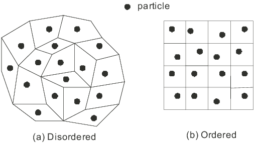
The non-uniform cell model in (a) for the disordered state is a generalization of the uniform cell model traditionally used in cell theories. The other difference is that we allow for an internal variable. The motion of each particle within its cell is governed by due to all its neighbor, which we denote by , where is the position of the particle under consideration within its cell and denotes the set of the positions of all its neighbors that are continually c hanging in time. The connectivity between the neighbors and the central molecule has to be properly accounted for in this set. This requires considering the probability for the potential . It is given by the following identity
where the prime over the sum implies that the sum is restricted to those microstates in which the particle and its cell neighbors are restricted to be at and .
It is obvious that the cell volume must be at least as big as needed to allow for the local oscillations. The local motion within the cell potential can be used to characterize a volume, which we will call the interaction volume of the particle: it is the minimum volume needed for the allowed local motion. One way to quantify is by the root-mean square-root of the displacement during the local motion as follows. The average over all possible cell potentials with probability of the displacement squared is given by
where is taken to be at the minimum of the potential in the inherent structure IS. The inner integral is over the time period of an oscillation controlled by . We first observe that the changes with the temperature. To see this most clearly, we simply consider an interparticle harmonic potential . From dimensional analysis alone, we conclude that the mean square displacement of all the particles scales as the temperature:, where is the spring constant of the potential. Thus,
Accordingly, it vanishes at absolute temperature . It usually happens that the oscillatory modes equilibrate rapidly with the medium. In that case, we must replace by . At absolute zero, particles are sitting in an IS, and there is an average distance between particles. Half of the average distance is taken as the ”radius” of the particle, which then determines its interaction volume at absolute zero. This is the minimum of the interaction volume. The distance should not be confused with the so-called radius of a particle corresponding to the ”impenetrability” of the particles.1010 10 The interparticle potential begins to rise steeply for separation between particles below the ”radius” [5]. Thus, not strictly the radius of a particle. As the temperature increases, the linear size of the particle increases due to oscillations and so does its interaction volume, which is now given by
in terms of a geometrical factor of order unity. The above volume may be quite different from the customarily defined occupied volume , which is commonly used in the glassy literature. Unfortunately, there is a lot of ambiguity in the definition of and how to obtain it theoretically [9] so we make no attempt to compare the two.
The difference is the remainder volume of the cell, called the free volume , that is the elbow room for the translation and rotation of the center of mass of the particle. This motion gives rise to the diffusion of the particle from the region over which the local oscillatory motion occurs. As decreases, the elbow room, i.e., increases (and so do and ) but not so much so that particles are still confined within their respective cells. As the free volume increases further, the particles can escape to the neighboring cells so that sometimes a cell may have multiple occupancy of the particles. The particles will undergo local motion in the new cell before they make excursion to another neighboring cell. If the free volume increases too much, then diffusion becomes the dominant motion and the local motion is no longer possible as the particles are far apart now. A situation like this occurs in gases. The above picture is an average picture so that it will also occur due to fluctuations in energy,volume, and internal variables. The aforementioned scenario has been confirmed by numerical simulations that has been discussed by several authors; see for example, Refs. [1, 13] and Fig. 1.
The above discussion is equally valid for the disordered and ordered macrostate. We will, however, consider the disordered macrostate in the following.
VI.2 The Hole Theory
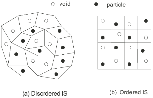
An obvious refinement of the above cell theory is to allow for holes in the theory; see (a) and (b) in Fig. 5. The empty sites refer to holes, that is, the absence of a particle and gives an additional contribution to the free volume in this theory. It also allows for a considerable variation in the number of neighboring particles due to the presence of holes, which makes this theory attractive. As the volume of a glass is found to be considerably greater than that of the corresponding crystal or ESCL, it is argued that the glass has a significant number of holes, which decreases during relaxation. In general, the decrease in the free volume is considered to be related to the irreversible relaxation, while the decrease in the interaction volume is argued to be related to the equilibrium relaxation as noted above since the local motion within the cell potential occurs at the temperature of the medium and not at the instantaneous temperature of the glass; see also the discussion by Matsuoka [9]. The division of volume in the interaction and free volumes results in the two volumes to be independent as they refer to independent degrees of freedom. Their existence may be related to the success of the two parameter model of Aklonis and Kovacs [14].
VI.3 Communal Entropy
Using the fact that entropy and volume are both extensive, we find that the entropy density is a homogeneous function of order zero, that is, it is not extensive. We can write the entropy as a sum of two terms: This is a trivial identity but allows us to introduce two different entropy components associated with the two components of the volume. One such component is , which is associated with the translation of the particles. The free volume decreases as increases and inhibits the translation. The particles must be fully jammed if there is no elbow room (). In this state, there cannot be any translation and must also vanish. This identifies the ideal glass (IG). If we wish to identify the communal entropy associated with the free volume, then it must vanish for the ideal glass. Thus, the relationship between and must be linear because of the extensivity. If we write it as with , then the other component , the interaction entropy, is given by . However, must be determined by the cell potential , which depends on or but is independent of the free volume. Hence, . Thus, we write
each of the above two components of the entropy must be non-negative and must satisfy the second law. As said earlier, includes the entropy associated with different conformations of the molecules. The communal entropy that plays a central role in the study of glasses [6, 11, 1]. The deep connection that we have discovered between the free volume and communal entropy shows that they vanish simultaneously in IG so that whether we vary the density (control variable ) or the entropy (control variable ), we obtain the unique IG at the respective Kauzmann point. This, we hope, will clarify some confusion present in the field as we discuss now.
VII Some Glass Transition Theories
We briefly review some important theories that have been used to explain glass transitions; for more details, see Ref. [6]. None of them at present is able to explain all observed features of glass transition [15, 16]. Thus, we are far from having a complete understanding of the phenomenon of glass transition, and it is fair to say that there yet exists no completely satisfying theory of the glass transition. Theoretical investigations mainly utilize two different approaches, which are based either on thermodynamic or on kinetic ideas, neither of which seems complete.

VII.1 Thermodynamic Approach: General Considerations
We first focus on our nonequilibrium approach to see what general conclusions can be drawn before considering other theories. In the following, we are interested in SCL state, which can be divided into two: time-dependent NESCL and time-independent ESCL in the restricted ensemble. We will focus on the communal entropy for which we use instead of for notational simplicity. We will exhibit and suppress all other extensive observables below and use a single internal variable for simplicity. According to the second law ; see Fig. 6. As the slope of FG determines the inverse of the internal temperature of NESCL, while that of DFCK the inverse of the medium temperature , we conclude from the figure that at is higher than at . Indeed, as at and at , where is the energy at F, it is evident that over FG. As has no singularity over its entire range KGF, we can expand in the form of a Taylor expansion over FG around the point K. For later applicability, it is useful to consider as a function of and . We will suppress in the following. In an isobaric vitrification at medium pressure , it is not hard to conceive that , which we will assume in the following. Introducing and and recognizing that at K the heat capacity is non-zero but finite and that the affinity vanishes, we immediately conclude that the leading terms in the expansion must be linear in (no linear term in ) and bilinear in . Thus, we can pull out from all the expansion terms to finally write in terms of a function whose definition is evident from the (infinite) Taylor expansion ():
| (23) |
we have not shown any dependence on as it is a function of so it is no longer independent. The extensive function takes the value . It must increase as decreases during isothermal relaxation to ensure that continues to increase.
A similar Taylor expansion can be made for the volume . We first recall that and the communal entropy vanish simultaneously1111 11 In contrast, there is no such relationship between the configurational entropy and the free volume. The most simple way to appreciate is to recognize that the configurational entropy in the Gibbs-Di Marzio theory can vanish even when the polymers cover the entire lattice so that the free volume is identically zero. and that
| (24) |
Thus, is also non-singular and will have a Taylor expansion around the Kauzmann point. To determine the nature of the expansion, we follow the above approach to determine the leading powers of and . The volume expansion coefficient at K due to the free volume is nonzero as we approach K from the high temperature side because of the difference in the slopes at K in Fig. 2. Thus, the expansion must start with a term linear in . The determination of the leading power of requires considering the behavior of . It follows from the theorem of small increments [5] that
where is the double Legendre transform 1212 12 should not be confused with the Gibbs free energy . This point is carefully discussed in Ref. [13]. so that . As the affinity always vanishes at K regardless of the pressure, the derivative on the right side must vanish. This means that must vanish at K, which leads to a leading bilinear combination . Thus, the situation is as before for so that we can write a similar form for
| (25) |
We can use this form of the free volume in the Doolittle equation (6) to obtain
| (26) |
in terms of the intensive function . It should be noted that all quantities above are functions of and . Using the linear relationship from (24) in (6), we obtain
| (27) |
in terms of the per particle communal entropy . Again, all quantities are functions of state variables.
VII.1.1 Free Volume Theory
The free volume theory of Doolittle [10, 11] attempts to describe both aspects with some respectable success even though lately it has fallen out of favor. This is unfortunate as this theory captures the essence of the GT, which in this theory occurs when the free volume becomes sufficiently small to impede the mobility of the molecules [10]. The Doolittle equation correctly predicts the abrupt increase in the viscosity for a large number of glass formers in a narrow range over which becomes very small; see ref. [11] for further details. The time-dependence of the free-volume redistribution, determined by the energy barriers encountered during redistribution, should provide a kinetic view of the transition, and must be properly accounted for. This approach is yet to be completed to satisfaction. Nevertheless, assuming that the change in free volume is proportional to the difference in the temperature near some temperature , it is found that diverges near according to the phenomenological Vogel-Tammann-Fulcher equation
| (28) |
where and are system-dependent constants. A comparison with (26) shows the phenomenological equation to be a special case of the general equation. The limited validity of the original (constant parameters) Doolittle equation also makes the VTF equation with limited validity. in addition, different concept of the free volume will also yield different temperatures where it vanishes. This explains the puzzling differences between and the Kauzmann temperature noted by several workers.
VII.1.2 Adam-Gibbs Theory
The thermodynamic theory due to Adam and Gibbs [17, 6] attempts to provide a justification of the entropy crisis in SCL. The central idea is that the sluggishness observed in a system is a manifestation of the smallness of the configurational entropy, i.e. the smallness of the available configurations to the system. The configurational entropy in this theory is identical to the configurational entropy defined above in (2). This entropy should not be confused with the communal entropy that we have been considering above. According to this theory, the viscosity above the glass transition is given as follows:
| (29) |
where and are system-dependent constants and . It is commonly believed that the configurational entropy also vanishes at a positive temperature , which is not identical to , although they are found to be close [11]. A similar argument as used above will also show that
where . The derivation of (29) is based on the concept of cooperative domains of size , which gradually increases as the temperature is lowered and diverges at . At this temperature, the entire system acts like a cooperative domain. While this particular domain is disordered, its configurational entropy must vanish in this theory. As the laboratory glass transition temperature occurs at about 50 K above , the value of at is much smaller; it is found to be of the order of .
If we replace in (29) by the communal entropy, then the above equation represents a special case of the general thermodynamic equation given in (27) except that the viscosity diverges at different temperatures in the two approaches. As the two theories are developed based on different approaches but with the same conclusion, it appears that the suggestion of a rapid rise in the viscosity due to a sudden drop in some form of entropy seems very enticing, since both phenomena are ubiquitous in glassy states. Thus, we are driven to the conclusion that we can treat the SCL glass transition within a thermodynamics formalism in which some sort of entropy crisis is exploited. While the vanishing of free volume is not tied to the vanishing of , the vanishing of free volume occurs simultaneously with the vanishing of the communal entropy. Thus, our approach exploiting the communal entropy ties the divergence of the viscosity with the vanishing of either the free volume or the communal entropy at the same temperature .
VII.2 Mode-Coupling Theory
The mode-coupling theory [18] is an example of theories based on kinetic ideas in which deals not with the glass transition but with the transition at Thus, it is not directly relevant for our review. This theory may be regarded as a theory based on first-principle approach, which starts from the static structure factor. In this theory, the ergodicity is lost completely, and structural arrest occurs at a temperature , which lies well above the customary glass transition temperature . Consequently, the correlation time and the viscosity diverge due to the caging effect. The diverging viscosity can be related to the vanishing free volume [11, 10], which might suggest that the MC transition is the same as the glass transition. This does not seem to be the consensus at present. It has been speculated that the divergence at is due to the neglect of any activated process in this theory. This, however, has been disputed by recent studies. The mode-coupling theory is also not well-understood, especially below the glass transition. More recently, it has been argued that this and mean-field theories based on an underlying first-order transition may be incapable of explaining dynamic heterogeneities.
VII.3 Random First Order Theory
An alternative thermodynamic theory for the impending entropy crisis based on spin-glass ideas has also been developed in which proximity to an underlying first-order transition is used to explain the glass transition [19]. The theory is based on the one-step replica symmetry breaking in spin glasses which also undergo a spin-glass transition similar in many respect to the freezing transition in glasses. The one-step replica symmetry breaking is identified in a long-range spin glass model so the theory is at a mean field level. While some may consider this to be a weakness of the theory, it also provides a new level of intuition about ordinary glasses.
VIII A Simple Model of a Non-equilibrium Temperature
The possibility of a temperature disparity can be heuristically demonstrated by considering a simple non-equilibrium laboratory problem. Consider a system as a “black box” consisting of two parts at different temperatures and , but insulated from each other so that they cannot come to equilibrium. The two parts are like slow and fast motions in a glass, and the insulation allows us to treat them as independent, having different temperatures. We assume that there are no irreversible processes that go on within each part so that there is no irreversible heat and generated within each part. We wish to identify the effective temperature of the system. To do so, we imagine that each part is added a certain infinitesimal amount of heat from outside, which we denote by and The amount of heat added to the system is their sum. We assume the entropy changes to be and . Then, we have
Let us introduce a temperature by . Using , we immediately find
By introducing , which is determined by the setup, we find that is given by
| (30) |
As is between and , it is clear that lies between and depending on the value of . Thus, we see from this heuristic model calculation that the effective temperature of the system is not the same as the temperature of either parts, a common property of a system not in equilibrium.
The above calculation is for fixed and since the infinitesimal heats do not change the temperatures and there is no energy exchange between the two parts due to insulation. It is the value of that uniquely determines the temperature of the system. It depends on the way the two heats are exchanged.
If the insulation between the parts is not perfect, there is going to be some energy transfer between the two parts, which would result in maximizing the entropy of the system. As a consequence, their temperatures will eventually become the same. During this time, the temperature of the system will lie between the changing temperatures of the two parts, and will itself be changing.
IX The Fictive Temperature and the Tool-Narayanaswamy Equation
We will exhibit in this section.
IX.1 Partitioning the Degrees of freedom (dof)
The relaxation of all thermodynamic properties in the temporal domain depends on the of the state of the system. For example, at high enough temperatures, the time variation of as it relaxes towards can be described as a single simple exponential with a characteristic time scale , the relaxation time. This happens when all the degrees of freedom (dof) come to equilibrium simultaneously with the same relaxation time. At any time before equilibrium is reached, the system has a temperature ; it also has energy etc.
At low temperatures, this is not true. There are slow and fast modes noted in Sect. I. The situation is similar to the simple system considered in Sect. VIII, which we now imagine to be in a medium at temperature . Both parts will strive to come to equilibrium with the medium but they may have widely separated relaxation times describing the fast and slow modes in the system. Situation similar to this also occurs in the attainment of thermal equilibrium between the nuclear spins and their environment during nuclear relaxation studied by Purcell, where the spin-lattice relaxation is extremely slow. The explanation of the slow and fast dof in a wide class of substances lies in internal molecular motions other than simple vibrations. The fast dof cool down and equilibrate very fast, while the slow dof take much longer to transfer their energy and equilibrate because of very weak coupling with the surrounding medium. We will denote those dof that have equilibrated with the medium at time by a subscript ”e”, and the remaining that are not equilibrated by ”n.”
Let denote the total number of the dof in the system, which is determined by the number of particles in it; hence, it remains constant. The fast dof equilibrate within the observation time with the slow dof remaining out of equilibrium [2]. Eventually, as , all dof come to equilibrium with the medium. Let and denote its partition in equilibrated and non-equilibrated dof, respectively:
evidently, they are functions of time. Assume that at the system is cooled instantaneously from an equilibrated supercooled liquid at to a glass state at . Immediately prior to cooling, all dof are in equilibrium at and for . At , all dof are out of equilibrium with the new medium at so that . Eventually, for all . It is clear that does not remain constant. Thus slow dof become part of in time,.
The weak coupling between the two dof and of the slow dof with the medium allows us to treat them as almost uncorrelated and quasi-independent, which then immediately leads to the following partition of the and into two contributions, one from each kind:
| (31) |
It should be noted that and stand for and
We have already remarked earlier that in (5) corresponds to during . During this time, the glass is trapped within an inherent structure IS0. The slow dof correspond to the center of mass motion within the cells and to visit other ISs. They are too slow to equilibrate at the new temperature. A large body of simulations discussed in Ref. [13] has established a very clear pattern for the mean square displacement of a particle as a function of time , starting from a ballistic regime to a plateau to a final diffusive regime; see also Zallen [1].
IX.2 Fictive State and Temperature
Let us now introduce
| (32) |
at a given , so that
| (33) | ||||
| (34) |
At , and At , and . As time goes on, more and more of the ”n” dof equilibrate, thus increasing and .
By definition, we have , while the dof will have a temperature different from this. Assuming internal equilibrium, we can introduce a new temperature by
| (35) |
The following identity
| (36) |
easily follows from considering and using (31) and (33). This equation should be compared with (30) obtained earlier using a heuristic model. Initially, so that , while as , as expected. This division of the instantaneous temperature into and is identical in form to that suggested by Narayanaswamy [2], except that we have given thermodynamic definitions of in (32) and in (35).
IX.2.1 Physical Significance
Let us now understand the significance of the above analysis. The partition in (31) along with the fraction shows that the partition satisfies a lever rule: the relaxing glass can be conceptually (but not physically) thought of as a ”mixture” consisting of two different ”components” corresponding to dof and dof: the former is at temperature and has a weight ; the latter with a complementary weight is at a temperature Thinking of a system conceptually as a ”mixture” of two ”components” is quite common in theoretical physics. One common example is that of a superfluid, which can be thought of as a ”mixture” of a normal viscous ”component” and a superfluid ”component”. In reality, there exist two simultaneous motions, one of which is ”normal” and the other one is ”superfluid”. A similar division can also be carried out in a superconductor: the total current is a sum of a ”normal current” and a ”superconducting current”.
IX.2.2 Nonequilibrium Aspects and A Fictive State
However, because of the non-equilibrium nature of the system, there is an important difference between a glass and a superfluid or a superconductor. The e-component is in equilibrium (with the medium), but the n-component is only in internal equilibrium. While the significance of the former as a ESCL ”component” at (dof=) is obvious, the significance of the latter requires clarification. At , of ESCL (dof=) from which the current glass is obtained so that . Also, and At any later time , represents the temperature associated with the energy and volume of the non-equilibrated ”component” of the glass and has a weight . This ”component,” being in internal equilibrium, can be identified as a fictive ESCL [dof=] at temperature of energy and In other words, the relaxing glass at any time can be considered as consisting of two ESCL ”components,” one at temperature [dof=] and the other one [dof=] at temperature . The temperature uniquely determines and of the corresponding fictive ESCL [dof=], which is in equilibrium with a medium at temperature . Consequently, is no longer an independent state variable for the fictive ESCL.
As the above fictive liquid at contains only (or mostly) the slow dof, it does not yet really represent a ESCL associated with the system at , as the former lacks dof, while the latter contains all dof. This does not pose any problem as the missing dof at are in equilibrium not only with the dof at , but also with a medium at . Thus, one can consider ”adding” these missing dof (dof=) to the fictive liquid, which now represents the equilibrated ESCL (dof=) at . This ESCL is not the same as the glass with its fictive , as the latter has its dof at while the ESCL has all of its dof at . However, all of their thermodynamic properties associated with dof must be the same, as their entropy function is the same for both liquids. Similarly, the ESCL ”component” at (dof=) should also be ”supplemented” by the missing dof to give rise to the equilibrated ESCL at (dof=).
IX.2.3 Fictive Temperature
We are now in a position to decide which of the temperatures and qualifies as the fictive temperature. We will identify this temperature to characterize only the non-equilibrated dof (with respect to the medium, but having internal equilibrium among themselves) in the system, though other definitions are also possible. As contains information about both kinds of dof, it is not the appropriate temperature to be identified as the fictive temperature. The temperature , on the other hand, depends only on non-equilibrated dof, and should be identified as the fictive temperature of the relaxing glass at time . This temperature is not the instantaneous temperature of the glass at this time, but represents the equilibrium temperature of the corresponding ESCL at .
IX.3 Tool-Narayanaswamy Phenomenology: Single Slow Relaxation
The viscosity keeps changing with time during relaxation but it remains the property of the system. Thus, it must depend not on , but on , the instantaneous temperature that characterizes the instantaneous state of the glass. Using an Arrhenius form for the viscosity, we have
| (37) |
the form conventionally identified as the phenomenological Tool-Narayanaswamy equation [2]. Here, and are some parameters of the system. From the discussion in Sec. VII.1, they must in general depend on and the affinity .
It should be noted that our definition of the fictive temperature makes it somewhat different from the conventional definition used in the literature [2], which takes different values for different quantities such as the enthalpy and the volume. While we do not discuss it here, we have discussed it elsewhere [13] that the above definition of the fictive temperature and is the same even if we use the partition of the volume instead of the energy. Therefore, we need to follow the consequences of this difference in their definition. This will require a particular model of the dynamics in the system. A common acceptable form is the Kohlrausch form in (4). The exponential itself may be taken to be a function of time and temperature to account for deviations seen at short times and long times . Usually, increases monotonically with the temperature. Thus, it will also change during relaxation as changes. Let us assume for the moment that our is not very different from the customary fictive temperature. Conventionally, the viscosity is fitted by taking as a constant close to , but allowing three other adjustable parameters ( and ) to obtain the best fit [2, see the contribution by Moynihan et al]; all parameters will generally have some time-dependence, but their time-dependence is neglected in finding the best fit. Indeed, even the values of the fictive temperature have appreciable uncertainties depending on the procedure to find it. Therefore, such fits do not rule out a slowly varying . Time-dependence of has been recognized for quite some time in the literature; see Ref. [13] for more details.
There cannot be any doubt that a constant in (37), that is being independent of the aging conditions, is an approximation when used to describe experiments. But this is most certainly not correct as no nonequilibrium state, in which and have different temperatures, can be identified with an equilibrium state with all dof at temperature . Recall that there is a unique relationship between and the temperature . However, there can be a variety of glasses with different energies but all having the same fictive temperature . Thus, the original idea of Tool cannot be correct. What our approach shows is that an ageing glass has two distinct dof and only the non-equilibrated dof should be identified with the equilibrated liquid at . This picture now no longer supports ageing-independent . This is where our new understanding differs from the original idea of Tool. This also makes data-fitting a challenge. This is the price to be paid for changing from an empirical parameter to a thermodynamic quantity. However, the benefit of our approach is that the fictive temperature is the same whether we consider the energy or the volume. It would be interesting to see what kind of time- and temperature-dependence will exhibit with our definition of the fictive temperature. This will require introducing a particular dynamics, which is not our aim in this paper.
The extension to more than one slow relaxation has been considered by us in Ref. [13] and will not be pursued here.
X Discussion and Conclusions
After giving a brief review of some of the important issues in vitrification and its phenomenology, we follow it up with a brief introduction to a recently developed non-equilibrium thermodynamics of a system in internal equilibrium and apply it to supercooled liquids and glasses. The concept of internal equilibrium requires the system to be homogeneous and its instantaneous entropy to be maximum for the state variables at that instant. The state variables include some internal variables that cannot be controlled by the observer. An inhomogeneous system also requires internal variables. A simple example of an internal variable for an inhomogeneous system is given, which is again considered to introduce the instantaneous temperature later in Sec. VIII. This model is central to justify the Tool-Narayanaswamy equation later.
The conventional approaches to study viscosity as a function of temperature either uses or . The Adam-Gibbs theory is based on instead of . (However, the two are not the same, at least for polymers. While the former contains the conformational entropy, it is absent in .) By replacing by , one can determine the temperature where the viscosity diverges in the Adam-Gibbs theory. In the free volume theory, the viscosity diverges at . The two temperatures are usually different as there is no relationship between the vanishing of and . This is puzzling as the state of the system is its thermodynamic property and is independent of the theory used to describe the system. Moreover, the state with a diverging viscosity must be a unique state in that once the viscosity has diverged, it cannot change in time. In general, for a system in internal equilibrium, the viscosity must be a function of the state variables: For a state with diverging viscosity, there cannot be any variations in the fields. In other words, we expect a unique temperature where diverges so that the above two temperatures must be the same. This mismatch is remedied by our approach in which we take the ideal glass state to be a unique state in which and vanish together so that the above two temperatures are not different from the Kauzmann temperature . Thus, the different looking (free volume and Adam-Gibbs) theories become identical as we have shown. This unification comes from the uniqueness of the ideal glass. Whether we ever get to the state is not relevant for the mathematical expansion around the Kauzmann point.
The nonequilibrium nature of SCL and GS requires that we make a distinction between the instantaneous fields and those of the medium. If this is not done, as is usually the case in most nonequilibrium approaches in which internal variables are introduced, then the Gibbs free energy does not change, while it must decrease during relaxation for a system out of equilibrium. Indeed, , etc. act as thermodynamic forces that drive the system towards equilibrium. These forces have some important consequences for how fields like , etc. and thermodynamic quantities like the volume, entropy, enthalpy, etc. change in time.
The actual form of the dynamics in time was not considered here as our interest was to understand how thermodynamic quantities change with fields. However, the nature of the dynamics was incorporated in an indirect way be realizing that the dynamics in SCL and GS should be divided into fast and slow dynamics. Based on this observation, it was necessary to divide and into two parts, depending on the fast modes ( and ) and slow modes ( and ). General considerations show that these quantities are linearly related. As a consequence, and vanish simultaneously in IG. As IG emerges out of ESCL, it is an equilibrium state in so that its fields are those of the medium. When the entropy of some NESCL is extrapolated to energies below , as was discussed in reference to Fig. 6, we argued that the extrapolated state of zero communal entropy must be IG; the local oscillatory motion in the cages are governed by equilibrium thermodynamics.
The linear relation associated with the free volume is different from alternate choice . We do not consider the latter choice as it gives negative communal entropy, whereas we have required it to non-negative.
We have clarified the concept of the fictive temperature widely used in the study of glasses by identifying it as a thermodynamic quantity; see (35). Our analysis shows that the fictive temperature has the same value even if we change the relaxing quantity from the energy to the volume. This temperature is not identical to but is related to the instantaneous temperature in a glass; see (36). We use this relationship to establish the Tool-Narayanaswamy equation (37) for the relaxation time on a solid theoretical ground. As we have been able to offer a thermodynamic interpretation of , it no longer is merely a parameter following the original idea of Tool. Therefore, it is not surprising that the time-dependence of requires reinterpreting Tool’s original idea of the fictive temperature. It should not be interpreted as the fictive temperature at which the glass is in equilibrium; rather, it is only the non-equilibrated dof of the glass that is compared with the equilibrium liquid at the fictive temperature .
The limitation of the paper should be mentioned. We have not discussed recent work dealing with the heterogeneity in space and time to discuss glasses. The reason for this is that the nonequilibrium thermodynamics that we are using requires the additivity of the entropy for different parts. This requires the parts to be macroscopically large so that surface effects can be neglected. Thus, the approach is not applicable to a few particles for which we need small size nonequilibrium thermodynamics, a field which is in infancy at present.
References
- [1] R. Zallen, The Physics of Amorphous Solids, John Wiley, New York (1983).
- [2] The Glass Transition and the Nature of the Glassy State, edited by M. Goldstein and R. Simha, N.Y. Academy of Sciences, New York (1976).
- [3] K. Fischer and J. Hertz, Spin Glasses, Cambridge University Press, Cambridge, U.K.; Reprint edition (1993).
- [4] W. Kauzmann, Chem. Rev., 43, 219-256 (1948).
- [5] L.D. Landau, E.M. Lifshitz, Statistical Physics, Part 1, Third Edition, Pergamon Press, Oxford (1986).
- [6] P.D. Gujrati in Modeling and Simulation in Polymers, edited by P.D. Gujrati and A.I. Leonov, Wiley-VCH, , Weinheim (2010).
- [7] P.D. Gujrati, arXiv:1304.3768; P.D. Gujrati, Entropy 17, 710 (2015).
- [8] K.L. Ngai in Soft Matter under Exogenic Impacts, S.J. Rzoska and V.A. Mazur, ed. p. 91, Springer (2007).
- [9] S. Matsuoka, Poly. Eng. Sci. 21, 907 (1981).
- [10] A.K. Doolittle, J. Appl. Phys. 22, 1471 (1951).
- [11] G.S. Grest and M.H. Cohen; Adv. Chem. Phys. 48, 455 (1981).
- [12] S.V. Nemilov, Thermodynamic and Kinetic Aspects of the Vitreous State, CRC, Boca Raton (1995).
- [13] P.D. Gujrati, Phys. Rev. E 81, 051130 (2010); P.D. Gujrati, arXiv:0910.0026.
- [14] J.J. Aklonis and A.J. Kovacs in Contemporary Topics in Polymer Science, M. Shen, ed. Vol. 3, p. 267 (1979).
- [15] P.G. Debenedetti, Metastable Liquids, Concepts and Principles; Priceton University Press: Princeton, NY, USA (1996).
- [16] P.G. Debenedetti and F.H. Stillinger, Nature 410, 259 (2001).
- [17] G. Adams and J.H. Gibbs, J. Chem. Phys. 43, 139 (1965).
- [18] W. Gotze and L. Sjogren, Rep. Prog. Phys. 55, 241(1992).
- [19] V. Lubchenko and P.G. Wolynes, Annu. Rev. Phys. Chem. 58:235 (2007).