^∗ Center for Quantum Mathematics and Physics and Department of Physics, University of California Davis, Davis, California, 95616, USA ^♭ Department of Theoretical Physics and History of Science, University of the Basque Country, Bilbao, 48080, Spain ^♮ IKERBASQUE, Basque Foundation for Science, Maria Diaz de Haro 3, Bilbao, 48013, Spain ^† Center for Gravitational Physics, Yukawa Institute for Theoretical Physics, Kyoto University, Kyoto 606-8502, Japan ^‡ International Research Unit of Advanced Future Studies, Kyoto University, Japan

We study the effect of a bubble wall on the entanglement entropy of a free massive scalar field between two causally disconnected open charts in de Sitter space. We assume there is a delta-functional wall between the open charts. This can be thought of as a model of pair creation of bubble universes in de Sitter space. We first derive the Euclidean vacuum mode functions of the scalar field in the presence of the wall in the coordinates that respect the open charts. We then derive the Bogoliubov transformation between the Euclidean vacuum and the open chart vacua that makes the reduced density matrix diagonal. We find that larger walls lead to less entanglement. Our result may be regarded as evidence of decoherence of bubble universes from each other. We also note an interesting relationship between our results and discussions of the black hole firewall problem.

1 Introduction

Quantum entanglement has fascinated many physicist because of its counterintuitive nature. Quantum entanglement makes it possible to know everything about a system composed of two subsystems (in a pure state) but know nothing at all about the subsystems (in the case of maximal entanglement). After Aspect et al. succeeded in showing experimental evidence of the quantum nature of entanglement by measuring correlations of linear polarizations of pairs of photons [1, 2], much attention has been paid to this genuine quantum property in various research areas including quantum information theory, quantum communication, quantum cryptography, quantum teleportation and quantum computation.

Quantum entanglement should play an important role in cosmology. In de Sitter space where the universe expands exponentially, any two mutually separated regions eventually become causally disconnected. This is most conveniently described by spanning open universe coordinates on two open charts in de Sitter space. The positive frequency mode functions of a free massive scalar field for the Euclidean vacuum (the Bunch-Davies vacuum) that have support on both regions were derived in [3]. Using them, quantum entanglement between two causally disconnected regions in de Sitter space was first studied by Maldacena and Pimentel [4]. They showed that the entanglement entropy, which is a measure of quantum entanglement, of a free massive scalar field between two disconnected open charts is non-vanishing. Motivated by this, the entanglement entropy of $\alpha$ -vacua [5, 6], that of the Dirac field [7] and axion field were examined [8, 9]. The spectrum of cosmological fluctuation was also studied in [10, 11]. Quantum entanglement is also of considerable interest in the context of the proposed “entanglement – geometry correspondence”(e.g. [12, 13]).

One of the cornerstones of inflationary cosmology is that primordial density fluctuations have a quantum mechanical origin. Inflation leads to an “initial state” of the universe following inflation which is highly entangled. This invites the question of whether compelling observational evidence for the entangled nature of the initial density fluctuations can be found. Several studies have been made on quantifying the initial state entanglement by using some measure of entanglement such as the Bell inequality [14, 15, 16, 17, 18, 19, 20], entanglement negativity [21, 22, 23] and quantum discord [24, 25]. There have also been several attempts to find some observational signatures on the CMB when the initial state is a non-Bunch-Davies vacuum due to entanglement between two scalar fields [26, 27], between two universes [28], and due to scalar-tensor entanglement [29, 30]

In this paper we extend the calculation of Maldacena and Pimentel [4] to the case where a bubble wall is present between the two open charts. The modes of the scalar field are changed by the presence of the wall, which in turn changes the entanglement entropy between the two regions. We find that for sufficiently large walls, the entanglement entropy approaches zero. Our technical results may prove useful in several of the areas discussed above. Here we focus on the possible implications for the decoherence of bubble universes.

The paper is organized as follows. In section 2, we review the method developed by Maldacena and Pimentel with some comments relevant to the calculation of the entanglement entropy with a bubble wall. In section 3, we introduce the bubble wall in the system and construct the positive frequency mode functions for the Bunch-Davies vacuum. We then compute the entanglement entropy and logarithmic negativity. Finally we summarize our result and discuss the implications in section 4.

2 Entanglement entropy in de Sitter space

Recently, Maldacena and Pimentel studied quantum entanglement between two causally disconnected regions in de Sitter space in [4]. They showed that the entanglement entropy of a free massive scalar field between two disconnected open charts is non-vanishing. In this section, we review their result.

2.1 Mode functions in the open chart

Figure 1: The Penrose diagram of the de Sitter space is shown.

L

and

R

are the two causally disconnected regions described by the open charts. A late-time spatial hypersurface in each region is depicted.

We consider a free scalar field $\phi$ with mass $m$ in de Sitter space represented by the metric $g_{\mu\nu}$ . The action is given by

\displaystyle S=\int d^{4}x\sqrt{-g}\left[\,-\frac{1}{2}\,g^{\mu\nu}\partial_{\mu}\phi\,\partial_{\nu}\phi-\frac{m^{2}}{2}\phi^{2}\,\right]\,.

(2.1)

The metric in each $R$ and $L$ region of open charts in de Sitter space (see Figure 1) can be obtained by analytic continuation from the Euclidean metric,

\displaystyle ds^{2}_{E}=H^{-2}\left[d\tau^{2}+\cos^{2}\tau\left(d\rho^{2}+\sin^{2}\rho\,d\Omega^{2}\right)\right]\,,

(2.2)

and expressed, respectively, as

	$\displaystyle ds^{2}_{R}$	$\displaystyle=$	$\displaystyle H^{-2}\left[-dt^{2}_{R}+\sinh^{2}t_{R}\left(dr^{2}_{R}+\sinh^{2}r_{R}\,d\Omega^{2}\right)\right]\,,$
	$\displaystyle ds^{2}_{L}$	$\displaystyle=$	$\displaystyle H^{-2}\left[-dt^{2}_{L}+\sinh^{2}t_{L}\left(dr^{2}_{L}+\sinh^{2}r_{L}\,d\Omega^{2}\right)\right]\,,$		(2.3)

where $H^{-1}$ is the Hubble radius and $d\Omega^{2}$ is the metric on the two-sphere. Note that the region $R$ and $L$ covered by the coordinates $(t_{L},r_{L})$ and $(t_{R},r_{R})$ respectively are the two causally disconnected open charts of de Sitter space¹¹ 1 The point between $R$ and $L$ regions is a part of the timelike infinity where infinite volume exists..

The solutions of the Klein-Gordon equation are expressed as

\displaystyle u_{\sigma p\ell m}(t,r,\Omega)\sim\frac{H}{\sinh t}\,\chi_{p,\sigma}(t)\,Y_{p\ell m}(r,\Omega)\,,\qquad-{\rm\bf L^{2}}Y_{p\ell m}=\left(1+p^{2}\right)Y_{p\ell m}\,,

(2.4)

where $(t,r)=(t_{R},r_{R})$ or $(t_{L},r_{L})$ and $Y_{p\ell m}$ are harmonic functions on the three-dimensional hyperbolic space. The eigenvalues $p$ normalized by $H$ take positive real values. The positive frequency mode functions corresponding to the Euclidean vacuum (the Bunch-Davies vacuum) that are supported both on the $R$ and $L$ regions are derived by Sasaki, Tanaka and Yamamoto in [3]:

\displaystyle\chi_{p,\sigma}(t)=\left\{\begin{array}[]{l}\frac{e^{\pi p}-i\sigma e^{-i\pi\nu}}{\Gamma(\nu+ip+\frac{1}{2})}P_{\nu-\frac{1}{2}}^{ip}(\cosh t_{R})-\frac{e^{-\pi p}-i\sigma e^{-i\pi\nu}}{\Gamma(\nu-ip+\frac{1}{2})}P_{\nu-\frac{1}{2}}^{-ip}(\cosh t_{R})\,,\\ \\ \frac{\sigma e^{\pi p}-i\,e^{-i\pi\nu}}{\Gamma(\nu+ip+\frac{1}{2})}P_{\nu-\frac{1}{2}}^{ip}(\cosh t_{L})-\frac{\sigma e^{-\pi p}-i\,e^{-i\pi\nu}}{\Gamma(\nu-ip+\frac{1}{2})}P_{\nu-\frac{1}{2}}^{-ip}(\cosh t_{L})\,,\end{array}\right.

where $P^{\pm ip}_{\nu-\frac{1}{2}}$ are the associated Legendre functions and the index $\sigma$ takes the values $\pm 1$ which distinguishes two independent solutions for each region, and $\nu$ is a mass parameter

\displaystyle\nu=\sqrt{\frac{9}{4}-\frac{m^{2}}{H^{2}}}\,.

(2.9)

Here and below in the text, we focus on the case $m^{2}/H^{2}<9/4$ to save space and make discussion clear. The extension to the case $m^{2}/H^{2}>9/4$ is straightforward, and the result we present will include both mass ranges.

Note that $\nu=1/2$ ( $m^{2}=2H^{2}$ ) is equivalent to a conformally coupled massless scalar. The minimally coupled massless limit is $\nu=3/2$ . For $1/2<\nu<3/2$ , it is known that there exists a supercurvature mode $p=ik$ where $0<k<1$ , which may be regarded as a bound-state mode. The role of supercurvature modes in the quantum entanglement is not clear. In [4], it is conjectured that they won’t contribute. In the body of this paper we simply ignore them. An analysis in the case of a conformal scalar in the presence of a bubble wall is given in the Appendix A. It turns out that a bubble wall can make the effective potential deep and allow a supercurvature mode to exist. In fact, we find that the eigenvalue $k$ can exceed unity and become arbitrarily large as the effective potential becomes deeper, and as a result the contribution of the supercurvature mode in the vacuum spectrum in each open chart is more important²² 2 See Eq. (3.10) in [31].

Going back to the solutions in Eq. (2.1), the Klein-Gordon normalization fixes the normalization factor as

\displaystyle N_{p}=\frac{4\sinh\pi p\,\sqrt{\cosh\pi p-\sigma\sin\pi\nu}}{\sqrt{\pi}\,|\Gamma(\nu+ip+\frac{1}{2})|}\,.

(2.10)

Since they form a complete orthonormal set of modes, the field can be expanded in terms of the creation and annihilation operators,

	$\displaystyle\hat{\phi}(t,r,\Omega)$	$\displaystyle=$	$\displaystyle\frac{H}{\sinh t}\int dp\sum_{\sigma,\ell,m}\left[\,a_{\sigma p\ell m}\,\chi_{p,\sigma}(t)+a_{\sigma p\ell-m}^{\dagger}\,\chi^{*}_{p,\sigma}(t)\,\right]Y_{p\ell m}(r,\Omega)$		(2.11)
		$\displaystyle=$	$\displaystyle\frac{H}{\sinh t}\int dp\sum_{\ell,m}\phi_{p\ell m}(t)Y_{p\ell m}(r,\Omega)\,,$		(2.11)

where $Y_{p\ell m}^{*}=Y_{p\ell-m}$ , $[a_{\sigma p\ell m},a_{\sigma^{\prime}p^{\prime}\ell^{\prime}m^{\prime}}^{\dagger}]=\delta(p-p^{\prime})\delta_{\sigma,\sigma^{\prime}}\delta_{\ell,\ell^{\prime}}\delta_{m,m^{\prime}}$ , and $a_{\sigma p\ell m}$ annihilates the Bunch-Davies vacuum, $a_{\sigma p\ell m}|0\rangle_{\rm BD}=0$ , and we introduced a Fourier mode field operator,

\displaystyle\phi_{p\ell m}(t)\equiv\sum_{\sigma}\left[\,a_{\sigma p\ell m}\,\chi_{p,\sigma}(t)+a_{\sigma p\ell-m}^{\dagger}\,\chi^{*}_{p,\sigma}(t)\right]\,.

(2.12)

For convenience, we write the mode functions and the associated Legendre functions of the $R$ and $L$ regions in a simple form $\chi_{p,\sigma}(t)\equiv\chi^{\sigma}$ , $P_{\nu-1/2}^{ip}(\cosh t_{R,L})\equiv P^{R,L}$ , $P_{\nu-1/2}^{-ip}(\cosh t_{R,L})\equiv P^{R*,L*}$ . Also below we omit the indices $p$ , $\ell$ , $m$ of $\phi_{p\ell m}$ , $a_{\sigma p\ell m}$ and $a_{\sigma p\ell-m}^{\dagger}$ for simplicity. For example, $a_{\sigma}=a_{\sigma p\ell m}$ and $a_{\sigma}^{\dagger}=a_{\sigma p\ell-m}$ unless there may be any confusion.³³ 3 It may be noted that this abbreviation implies $(a_{\sigma})^{\dagger}=a_{\sigma p\ell m}^{\dagger}\neq a_{\sigma}^{\dagger}=a_{\sigma p\ell-m}^{\dagger}$ . But since this is a small technical problem that can be easily solved by doubling the degrees of freedom, below we assume $(a_{\sigma})^{\dagger}=a_{\sigma}^{\dagger}$ .

2.2 Bogoliubov transformations and entangled states

Next we consider the positive frequency mode functions for the $R$ or $L$ vacuum that have support only on the $R$ or $L$ region, respectively. They are given by

\displaystyle\varphi^{q}=\left\{\begin{array}[]{ll}\tilde{N}_{p}^{-1}P^{q}&\mbox{in region}~q\,,\\ 0&\mbox{in the opposite region}\,,\end{array}\right.\quad\tilde{N}_{p}=\frac{\sqrt{2p}}{|\Gamma(1+ip)|}\,,

where $q=(R,L)$ . As the Fourier mode field operator (2.12) should be the same under this change of mode functions, we have

\displaystyle\phi(t)=a_{\sigma}\,\chi^{\sigma}+a_{\sigma}^{\dagger}\,\chi^{\sigma}{}^{*}=b_{q}\,\varphi^{q}+b_{q}^{\dagger}\,\varphi^{q}{}^{*}\,,

(2.16)

where we have introduce the new creation and annihilation operators ( $b_{q},b_{q}^{\dagger}$ ) such that $b_{q}|0\rangle_{q}=0$ . The operators $(a_{\sigma},a_{\sigma}^{\dagger})$ and $(b_{q},b_{q}^{\dagger})$ are related by a Bogoliubov transformation. The Bunch-Davies vacuum may be constructed from the states over $|0\rangle_{q}$ as

\displaystyle|0\rangle_{\rm BD}\propto\exp\left(\frac{1}{2}\sum_{i,j=R,L}m_{ij}\,b_{i}^{\dagger}\,b_{j}^{\dagger}\right)|0\rangle_{R}|0\rangle_{L}\,,

(2.17)

where $m_{ij}$ is a symmetric matrix. The condition $a_{\sigma}|0\rangle_{\rm BD}=0$ determines $m_{ij}$ :

\displaystyle m_{ij}=e^{i\theta}\frac{\sqrt{2}\,e^{-p\pi}}{\sqrt{\cosh 2\pi p+\cos 2\pi\nu}}\left(\begin{array}[]{cc}\cos\pi\nu&i\sinh p\pi\\ i\sinh p\pi&\cos\pi\nu\\ \end{array}\right)\,,

where $e^{i\theta}$ contains all unimportant phase factors for $\nu^{2}>0$ . This is an entangled state of the ${\cal H}_{R}\otimes{\cal H}_{L}$ Hilbert space.

The density matrix $\rho=|0\rangle_{\rm BD}\,{}_{\rm BD}\langle 0|$ is not diagonal in the $|0\rangle_{R}|0\rangle_{L}$ basis unless $\nu=1/2$ or $3/2$ . To make the calculation easier for tracing out the degrees of freedom in, say, the $L$ space later, we perform a further Bogoliubov transformation in each of $R$ and $L$ region. Apparently, this Bogoliubov transformation does not mix the operators in ${\cal H}_{R}$ space and those in ${\cal H}_{L}$ space. We introduce new operators $c_{q}=(c_{R},c_{L})$ that satisfy

\displaystyle c_{R}=u\,b_{R}+v\,b_{R}^{\dagger}\,,\qquad c_{L}=u^{*}\,b_{L}+v^{*}\,b_{L}^{\dagger}\,,

(2.21)

to obtain

\displaystyle|0\rangle_{\rm BD}=N_{\gamma_{p}}^{-1}\exp\left(\gamma_{p}\,c_{R}^{\dagger}\,c_{L}^{\dagger}\,\right)|0\rangle_{R^{\prime}}|0\rangle_{L^{\prime}}\,.

(2.22)

Note that the condition $|u|^{2}-|v|^{2}=1$ is assumed so that the new operators satisfy the commutation relation $[c_{i},(c_{j})^{\dagger}]=\delta_{ij}$ . The normalization factor $N_{\gamma_{p}}$ is given by

\displaystyle N_{\gamma_{p}}^{2}=\left|\exp\left(\gamma_{p}\,c_{R}^{\dagger}\,c_{L}^{\dagger}\,\right)|0\rangle_{R^{\prime}}|0\rangle_{L^{\prime}}\right|^{2}=\frac{1}{1-|\gamma_{p}|^{2}}\,,

(2.23)

where $|\gamma_{p}|<1$ should be satisfied. The consistency relations from Eq. (2.22) ( $c_{R}|0\rangle_{\rm BD}=\gamma_{p}\,c_{L}^{\dagger}|0\rangle_{\rm BD}$ , $c_{L}|0\rangle_{\rm BD}=\gamma_{p}\,c_{R}^{\dagger}|0\rangle_{\rm BD}$ ) give

\displaystyle\gamma_{p}=\frac{1}{2\zeta}\left[-\omega^{2}+\zeta^{2}+1-\sqrt{\left(\omega^{2}-\zeta^{2}-1\right)^{2}-4\zeta^{2}}\,\right]\,,

(2.24)

where we defined $\omega\equiv m_{RR}=m_{LL}$ and $\zeta\equiv m_{RL}=m_{LR}$ in Eq. (2.2). Note that a minus sign in front of the square root term is taken to make $\gamma_{p}$ converge. Putting the $\omega$ and $\zeta$ defined in Eq. (2.2) into Eq. (2.24), we obtain

\displaystyle\gamma_{p}=i\frac{\sqrt{2}}{\sqrt{\cosh 2\pi p+\cos 2\pi\nu}+\sqrt{\cosh 2\pi p+\cos 2\pi\nu+2}}\,.

(2.25)

Note that $\gamma_{p}$ simplifies to $|\gamma_{p}|=e^{-\pi p}$ for $\nu=1/2$ (conformal) and $\nu=3/2$ (massless). The $u$ and $v$ may be determined by inserting the above $\gamma_{p}$ into the consistency conditions.

2.3 Reduced density matrix and entanglement entropy

Given the density matrix in the diagonalized form, it is straightforward to obtain the reduced density matrix. From Eqs. (2.22) and (2.23), we obtain the density matrix for each mode labeled by $p,\ell,m$ as

\displaystyle\rho_{R}={\rm Tr}_{L}\,|0\rangle_{\rm BD}\,{}_{\rm BD}\langle 0|=\left(1-|\gamma_{p}|^{2}\,\right)\sum_{n=0}^{\infty}|\gamma_{p}|^{2n}\,|n;p\ell m\rangle\langle n;p\ell m|\,,

(2.26)

where we defined $|n;p\ell m\rangle=1/\sqrt{n!}\,(c_{R}^{\dagger})^{n}\,|0\rangle_{R^{\prime}}$ . In the conformal ( $\nu=1/2$ ) and massless ( $\nu=3/2$ ) cases, the reduced density matrix reduces to a thermal state with temperature $T=H/(2\pi)$ .

The entanglement entropy for each mode is given by

\displaystyle S(p,\nu)=-{\rm Tr}\,\rho_{R}(p)\log_{2}\rho_{R}(p)=-\log_{2}\left(1-|\gamma_{p}|^{2}\right)-\frac{|\gamma_{p}|^{2}}{1-|\gamma_{p}|^{2}}\log_{2}|\gamma_{p}|^{2}\,.

(2.27)

Then the total entanglement entropy between two causally disconnected open regions is obtained by integrating over $p$ and a volume integral over the hyperboloid,

\displaystyle S(\nu)=V_{H^{3}}^{\rm{reg}}\int_{0}^{\infty}\frac{dp\,p^{2}}{2\pi^{2}}S(p,\nu)=\frac{1}{\pi}\int_{0}^{\infty}dp\,p^{2}S(p,\nu)\,,

(2.28)

where $V_{H^{3}}^{\rm{reg}}=2\pi$ is the regularized volume of the hyperboloid [4]. The result is plotted in Figure 2. We see that the entanglement is largest for small mass (positive $\nu^{2}$ ) and decays exponentially for large mass (negative $\nu^{2}$ ). The two peaks correspond to the massless ( $\nu=3/2$ ) and conformal ( $\nu=1/2$ ) cases.

Refer to caption — Figure 2: Plot of the entanglement entropy normalized by the conformal scalar case ( $\nu=1/2$ ) as a function of $\nu^{2}$ .

3 Effects of a bubble wall on the entanglement

Now we study the effect of a bubble wall on the entanglement. The Penrose diagram of our setup is depicted in Figure 3. We consider the same action as Eq. (2.1) but now with $m^{2}$ as a function of the background geometry which contains a wall. In the case when the background geometry is given by an instanton solution with $\sigma(\tau)$ being the scalar field configuration and $\phi$ being its fluctuations, $m^{2}$ will be given by

\displaystyle m^{2}(\tau)=\frac{d^{2}V(\sigma)}{d\sigma^{2}}\,,

(3.1)

where $V$ is the potential of the $\sigma$ field, and the $\tau$ -dependence of $m^{2}$ is through its $\sigma$ -dependence. In a realistic situation, $m^{2}$ would be a smooth function of $\tau$ , and is positive on both sides of the wall, but negative at the wall where the potential has a peak. For simplicity, however, here we model the wall with a delta-function.

3.1 Setup

We consider the same action as Eq. (2.1) but now with a delta-functional wall in region $C$ parameterized by $\Lambda$ according to,

\displaystyle S=\int d^{4}x\sqrt{-g}\left[\,-\frac{1}{2}\,g^{\mu\nu}\partial_{\mu}\phi\,\partial_{\nu}\phi-\frac{m^{2}-\Lambda\delta(t_{C})}{2}\,\phi^{2}\,\right]\,.

(3.2)

where the metric is expressed as

\displaystyle ds^{2}_{C}

\displaystyle=

\displaystyle H^{-2}\left[dt_{C}^{2}+\cos^{2}t_{C}\left(-dr_{C}^{2}+\cosh^{2}r_{C}\,d\Omega^{2}\right)\right]\,.

(3.3)

Note that the radial coordinate $t_{C}$ in the region $C$ coincides with $\tau$ of the instanton solution (see Eq. (3.2.1) below). Note also that if we denote the width of the wall by $\Delta\tau_{w}$ , we have $\Lambda=|d^{2}V/d\sigma^{2}|H\Delta\tau_{w}$ .

Setting the field $\phi$ as

\displaystyle\phi=\frac{H}{\cos t_{C}}\chi_{p}(t_{C})Y_{p\ell m}(r_{C},\Omega)\,,

(3.4)

the solution of the mode function $\chi_{p}$ in the $C$ region is given by the associated Legendre function, $\chi_{p}\propto P^{\pm ip}_{\nu-\frac{1}{2}}(\sin t_{C})$ .

3.2 Mode functions in the presence of a wall

Now we want to pick up the positive frequency mode functions which are relevant for the pair creation of bubble universes through false vacuum decay. Namely, those mode functions that describe the Euclidean vacuum in the presence of a wall in region $C$ . They are obtained by requiring regularity in the lower hemisphere of the Euclidean de Sitter space with the wall when they are analytically continued to that region [3, 31].

3.2.1 The relation between the Lorentzian and the Euclidean coordinates

The open chart is obtained by analytic continuation of the Euclidean sphere $S^{4}$ . The Lorentzian coordinates of the regions $L$ , $R$ and $C$ are related to the Euclidean coordinates given in Eq. (2.2) as

\displaystyle\left\{\begin{array}[]{l}t_{R}=i\left(\tau-\frac{\pi}{2}\right)\hskip 62.59596pt\,,t_{R}\geq 0\\ r_{R}=i\rho\hskip 99.58464pt\,,r_{R}\geq 0\end{array}\right.

\displaystyle\left\{\begin{array}[]{l}t_{C}=\tau\hskip 71.13188pt\,,-\frac{\pi}{2}\leq t_{C}\leq\frac{\pi}{2}\\ r_{C}=i\left(\rho-\frac{\pi}{2}\right)\hskip 28.45274pt\,,0\leq r_{C}\leq\infty\end{array}\right.

\displaystyle\left\{\begin{array}[]{l}t_{L}=i\left(-\tau-\frac{\pi}{2}\right)\hskip 56.9055pt\,,t_{L}\geq 0\\ r_{L}=i\rho\hskip 102.43008pt\,,r_{L}\geq 0\end{array}\right.

For simplicity, we write $\sin t_{C}\equiv z_{C}$ , $\cosh t_{R}\equiv z_{R}$ , and $\cosh t_{L}\equiv-z_{L}$ below. Then, the above relations give $z_{C}=z_{R}=-z_{L}$ .

3.2.2 Analytic continuation in the presence of the wall

Let $\chi_{p}^{R}(z_{R})=P^{ip}_{\nu-\frac{1}{2}}(z_{R})$ and $\chi_{p}^{L}(z_{L})=P^{ip}_{\nu-\frac{1}{2}}(z_{L})$ ( $z_{L}=-z_{R}$ ) where

\displaystyle P^{\mu}_{\nu}(z)=\frac{1}{\Gamma(1-\mu)}\left(\frac{z+1}{z-1}\right)^{\frac{\mu}{2}}F\left(-\nu,\nu+1,1-\mu;\frac{1-z}{2}\right)\,;\quad z>1~\mbox{or}~z<-1\,.

(3.14)

$\bullet$ From $R$ ( $R=\{z_{R}>1\}$ ) to $C^{+}$ ( $C^{+}=\{0<z_{C}<1\}$ ):

Analytic continuation is through $\Im z_{R}<0$ . This means that the argument of $z_{R}-1=z_{C}-1$ is $-\pi$ . Hence $z_{R}-1=z_{C}-1=e^{-i\pi}(1-z_{C})$ . Thus

\displaystyle(1+z_{C})=(1+z_{R})\,,\quad(1-z_{C})=|1-z_{R}|e^{i\pi}=(z_{R}-1)e^{i\pi}\,,

(3.15)

which gives

\displaystyle\left(\frac{1+z_{R}}{z_{R}-1}\right)^{i\frac{p}{2}}=e^{-\frac{\pi}{2}p}\left(\frac{1+z_{C}}{1-z_{C}}\right)^{i\frac{p}{2}}\,,

(3.16)

when analytically continued from $z_{R}>1$ to $z_{R}=z_{C}<1$ . This means

\displaystyle\chi_{p}^{R}(z_{C})=e^{-\frac{\pi}{2}p}\,\tilde{P}^{ip}_{\nu-\frac{1}{2}}(z_{C})\,,

(3.17)

for $z_{R}=z_{C}<1$ , where $\tilde{P}^{\mu}_{\nu}(x)$ for $-1<x<1$ is defined as

\displaystyle\tilde{P}^{\mu}_{\nu}(x)=\frac{1}{\Gamma(1-\mu)}\left(\frac{1+x}{1-x}\right)^{\frac{\mu}{2}}F\left(-\nu,\nu+1,1-\mu;\frac{1-x}{2}\right)\,.

(3.18)

$\bullet$ From $C^{+}$ to $C^{-}$ ( $C^{-}=\{-1<z_{C}<0\}$ ):

Assuming there is a delta-functional wall of height $\Lambda$ at $z_{C}=0$ , $\chi_{p}^{R}(z_{C})$ is deformed to

\displaystyle\chi_{p}^{R}(z_{C})=e^{\frac{\pi}{2}p}\left(A_{p}e^{-\pi p}\tilde{P}^{ip}_{\nu-\frac{1}{2}}(z_{C})+B_{p}e^{\pi p}\tilde{P}^{-ip}_{\nu-\frac{1}{2}}(z_{C})\right)\,,

(3.19)

in $C^{-}$ , where $A_{p}$ and $B_{p}$ are given by

	$\displaystyle A_{p}$	$\displaystyle=$	$\displaystyle 1+\frac{\pi}{2i\sinh\pi p}\frac{\Lambda}{H^{2}}\|\tilde{P}^{ip}_{\nu-\frac{1}{2}}(0)\|^{2}\,,$		(3.20)
	$\displaystyle B_{p}$	$\displaystyle=$	$\displaystyle-\frac{\pi}{2i\sinh\pi p}\frac{\Lambda}{H^{2}}e^{-2\pi p}\left(\tilde{P}^{ip}_{\nu-\frac{1}{2}}(0)\right)^{2}\,.$		(3.21)

Note that in the absence of a wall ( $\Lambda=0$ ), we have $A_{p}=1$ and $B_{p}=0$ .

$\bullet$ From $L$ ( $L=\{z_{L}<-1\}$ ) to $C^{-}$ ( $C^{-}=\{-1<z_{C}<0\}$ ):

Now we express the above solution in terms of $\chi^{L}_{p}$ . To do this, we first introduce $\hat{z}_{C}=-z_{C}$ and analytically continue $\chi^{L}_{p}$ from $L$ to $C^{-}$ where $0<\hat{z}_{C}<1$ . Exactly the same as the analytic continuation from $R$ to $C^{+}$ , we have

\displaystyle\chi_{p}^{L}(\hat{z}_{C})=e^{-\frac{\pi}{2}p}\tilde{P}^{ip}_{\nu-\frac{1}{2}}(\hat{z}_{C})\,,

(3.22)

for $z_{L}=\hat{z}_{C}<1$ .

$\bullet$ matching $\chi^{R}$ with $\chi^{L}$ :

We now express $\chi^{R}_{p}$ in terms of $\chi^{L}_{p}$ and $\chi^{L}_{-p}$ . To do this, we express $P^{\pm ip}_{\nu-\frac{1}{2}}(z_{C})=P^{\pm ip}_{\nu-\frac{1}{2}}(-\hat{z}_{C})$ in terms of $P^{\pm ip}_{\nu-\frac{1}{2}}(\hat{z}_{C})$ , which can be achieved by using the transformation formulas for the hypergeometric functions in Appendix B. We find

\displaystyle P^{ip}_{\nu-\frac{1}{2}}(-\hat{z}_{C})=C_{p}\,P^{ip}_{\nu-\frac{1}{2}}(\hat{z}_{C})+D_{p}\,P^{-ip}_{\nu-\frac{1}{2}}(\hat{z}_{C})\,,

(3.23)

where

\displaystyle C_{p}=\frac{\cos\pi\nu}{i\sinh\pi p}\,,\qquad D_{p}=-e^{-2\pi p}\,\frac{\cos\left(\nu+ip\right)\pi}{i\sinh\pi p}\frac{\Gamma\left(\frac{1}{2}+\nu+ip\right)}{\Gamma\left(\frac{1}{2}+\nu-ip\right)}\,.

(3.24)

Using (3.23), $\chi^{R}_{p}$ is expressed as⁴⁴ 4 In the language of [31], we have $\displaystyle\alpha_{p}=e^{\pi p}\left(A_{p}D_{p}+B_{p}C_{-p}\right)\,,\quad\beta_{p}=A_{p}C_{p}+B_{p}D_{-p}\,.$ (3.25) We can check the symmetry, $\alpha^{*}_{p}=e^{-2\pi p}\alpha_{-p}\,,~\beta^{*}_{p}=\beta_{-p}\,.$

	$\displaystyle\chi^{R}_{p}(z_{C})$	$\displaystyle=$	$\displaystyle e^{\frac{\pi}{2}}\left[A_{p}\,P^{ip}_{\nu-\frac{1}{2}}(-\hat{z}_{C})+B_{p}\,P^{-ip}_{\nu-\frac{1}{2}}(-\hat{z}_{C})\right]$		(3.26)
		$\displaystyle=$	$\displaystyle\left(A_{p}C_{p}+B_{p}D_{-p}\right)\chi^{L}_{p}(\hat{z}_{C})+e^{\pi p}\left(A_{p}D_{p}+B_{p}C_{-p}\right)\chi^{L}_{-p}(\hat{z}_{C})\,.$		(3.26)

Notice that $P^{-ip}_{\nu-\frac{1}{2}}(-\hat{z}_{C})$ is not complex conjugate of $P^{ip}_{\nu-\frac{1}{2}}(-\hat{z}_{C})$ .

3.2.3 The Euclidean vacuum in the presence of the wall

Finally, the positive frequency mode functions for the Euclidean vacuum in the presence of the bubble wall are found to be

	$\displaystyle\chi_{p}^{R}(z)$	$\displaystyle=$	$\displaystyle\frac{1}{N_{w}}\left\{\begin{array}[]{l}P_{\nu-\frac{1}{2}}^{ip}(z_{R})\,,\\ \\ \left(A_{p}C_{p}+B_{p}D_{-p}\right)P_{\nu-\frac{1}{2}}^{ip}(z_{L})+e^{\pi p}\left(A_{p}D_{p}+B_{p}C_{-p}\right)P_{\nu-\frac{1}{2}}^{-ip}(z_{L})\,,\end{array}\right.$
	$\displaystyle\chi_{p}^{L}(z)$	$\displaystyle=$	$\displaystyle\frac{1}{N_{w}}\left\{\begin{array}[]{l}\left(A_{p}C_{p}+B_{p}D_{-p}\right)P_{\nu-\frac{1}{2}}^{ip}(z_{R})+e^{\pi p}\left(A_{p}D_{p}+B_{p}C_{-p}\right)P_{\nu-\frac{1}{2}}^{-ip}(z_{R})\,,\\ \\ P_{\nu-\frac{1}{2}}^{ip}(z_{L})\,,\end{array}\right.$

where the Klein-Gordon normalization for the above solutions is

\displaystyle N_{w}^{2}=\tilde{N_{p}}^{2}\left(1+|f_{p}|^{2}-|g_{p}|^{2}\right)\,,

(3.35)

where $\tilde{N}_{p}$ is defined in Eq. (2.2) and we have defined

\displaystyle f_{p}=A_{p}C_{p}+B_{p}D_{-p}\,,\qquad g_{p}=e^{\pi p}\left(A_{p}D_{p}+B_{p}C_{-p}\right)\,.

(3.36)

Note that in the absence of the wall ( $\Lambda=0$ ), we have $f_{p}=C_{p}$ and $g_{p}=e^{\pi p}D_{p}$ .

3.3 Bogoliubov transformations and entangled states

We perform the same Bogoliubov transformation in Eq. (2.16) that mixes the operators in the Hilbert spaces ${\cal H}_{R}$ and ${\cal H}_{L}$ . The derivation of the symmetric matrix $m_{ij}$ is given in Appendix C. The components of the $m_{ij}$ in Eq. (2.2) is now expressed as

	$\displaystyle\omega$	$\displaystyle=$	$\displaystyle-F\left[\left(f_{p}+f_{p}^{}\right)\left(1-\frac{\|g_{p}\|^{2}}{1-f_{p}^{2}}\right)-\left(1+\|f_{p}\|^{2}-\|g_{p}\|^{2}\right)\left(f_{p}-\frac{f_{p}^{}\|g_{p}\|^{2}}{1-f_{p}^{2}}\right)\right]\,,\qquad$		(3.37)
	$\displaystyle\zeta$	$\displaystyle=$	$\displaystyle-F\left[\left(f_{p}+f_{p}^{}\right)\left(f_{p}-\frac{f_{p}^{}\|g_{p}\|^{2}}{1-f_{p}^{2}}\right)-\left(1+\|f_{p}\|^{2}-\|g_{p}\|^{2}\right)\left(1-\frac{\|g_{p}\|^{2}}{1-f_{p}^{2}}\right)\right]\,,\qquad$		(3.38)

where

\displaystyle F=\frac{g_{p}^{*}}{1-f_{p}^{*2}}\frac{1}{E}\,,\qquad E=\left(1-\frac{|g_{p}|^{2}}{1-f_{p}^{*2}}\right)^{2}-\left(f_{p}-\frac{f_{p}^{*}|g_{p}|^{2}}{1-f_{p}^{*2}}\right)^{2}\,.

(3.39)

If there is no wall, $\omega$ is real ( $\omega=\omega^{*}$ ) and $\zeta$ is pure imaginary ( $\zeta=-\zeta^{*}$ ) for positive $\nu^{2}$ , then the second Bogoliubov transformation was simplified as in Eq. (2.21). In the presence of the wall, however, Eqs (3.37) and (3.38) are not real and pure imaginary respectively for positive $\nu^{2}$ . In this case, we need to perform the Bogoliubov transformation of the form

\displaystyle c_{R}=u\,b_{R}+v\,b_{R}^{\dagger}\,,\qquad c_{L}=\bar{u}\,b_{L}+\bar{v}\,b_{L}^{\dagger}\,,

(3.40)

to get the relation Eq. (2.22). Note that $|u|^{2}-|v|^{2}=1$ and $|\bar{u}|^{2}-|\bar{v}|^{2}=1$ are assumed. Then the consistency relations ( $c_{R}|0\rangle_{\rm BD}=\gamma_{p}\,c_{L}^{\dagger}|0\rangle_{\rm BD}$ , $c_{L}|0\rangle_{\rm BD}=\gamma_{p}\,c_{R}^{\dagger}|0\rangle_{\rm BD}$ ) give the system of four homogeneous equations

	$\displaystyle\omega\,u+v-\gamma_{p}\,\zeta\,\bar{v}^{}=0\,,\qquad\zeta\,u-\gamma_{p}\,\bar{u}^{}-\gamma_{p}\,\omega\,\bar{v}^{*}=0\,,$
	$\displaystyle\omega\,\bar{u}+\bar{v}-\gamma_{p}\,\zeta\,v^{}=0\,,\qquad\zeta\,\bar{u}-\gamma_{p}\,u^{}-\gamma_{p}\,\omega\,v^{*}=0\,.$		(3.41)

In order to have a non-trivial solution in the above system of equations, $\gamma_{p}$ must be [5]

	$\displaystyle\|\gamma_{p}\|^{2}$	$\displaystyle=$	$\displaystyle\frac{1}{2\|\zeta\|^{2}}\left[-\omega^{2}\zeta^{2}-\omega^{2}\zeta^{2}+\|\omega\|^{4}-2\|\omega\|^{2}+1+\|\zeta\|^{4}\right.$		(3.42)
			$\displaystyle\qquad\quad\left.-\sqrt{\left(\omega^{2}\zeta^{2}+\omega^{2}\zeta^{2}-\|\omega\|^{4}+2\|\omega\|^{2}-1-\|\zeta\|^{4}\right)^{2}-4\|\zeta\|^{4}}\,\right]\,,$		(3.42)

where we took a minus sign in front of the square root term to reduce Eq. (2.24) when there is no wall. Then putting Eqs. (3.37) and (3.38) into Eq. (3.42), we can calculate the entanglement entropy for each mode in Eq. (2.27). The resulting total entanglement entropy, Eq. (2.28), is plotted in Figure 4.

3.4 Entanglement entropy

From the left panel in Figure 4, we see that the entanglement entropy decreases as the effect of the wall increases for small mass (positive $\nu^{2}$ ). For large mass (negative $\nu^{2}$ ), the entanglement entropy decays exponentially in the absence of the wall ( $\Lambda=0$ ). In the presence of the wall, the peak at the conformally coupled scalar ( $\nu=1/2$ ) shifts to the left and eventually disappears as the effect of the wall increases. The right panel also shows that the peak of the entanglement entropy corresponding to the massless case and the conformally coupled scalar is an identical value in the absence of the wall ( $\Lambda=0$ ). However, as the effect of the wall becomes large, the entanglement entropy in the case of conformally coupled scalar decays faster than that of massless case.

3.5 Logarithmic negativity

In order to characterize the entanglement of a quantum state, there have been many entanglement measures proposed. The logarithmic negativity is one such measure of quantum entanglement. This measure is derived from the positive partial transpose criterion for separability [32]. The idea of it is to characterize an entangled state as a state that is not separable. In this subsection, we compute the entanglement of our model with the logarithmic negativity.

The second Bogoliubov transformation Eq. (2.22) is rewritten as

\displaystyle|0\rangle_{\rm BD}=N_{\gamma_{p}}^{-1}\sum_{n=0}^{\infty}\gamma_{p}^{n}\,|n;p\ell m\rangle_{R^{\prime}}|n;p\ell m\rangle_{L^{\prime}}\,,

(3.43)

where the states $|n;p\ell m\rangle_{R^{\prime}}$ and $|n;p\ell m\rangle_{L^{\prime}}$ are $n$ particle excitation states in $R^{\prime}$ and $L^{\prime}$ spaces. For a pure state, any state has a Schmidt decomposition expressed as

\displaystyle|\psi\rangle=\sum_{i}\sqrt{\lambda_{i}}\,|i\rangle_{A}\otimes|i\rangle_{B}\,,

(3.44)

where $\lambda_{i}$ is the probability to observe the $i$ th state and satisfies $\sum_{i}\lambda_{i}=1$ . By using the eigenvalues, the logarithmic negativity is expressed as

\displaystyle L{\cal N}=2\log_{2}\left(\sum_{i}\sqrt{\lambda_{i}}\right)\,.

(3.45)

Thus, if we compare Eq. (3.43) with the Schmidt decomposition, we can read off the corresponding eigenvalues

\displaystyle\sqrt{\lambda_{i}}=N_{\gamma_{p}}^{-1}|\gamma_{p}|^{n}\,,

(3.46)

and the logarithmic negativity for each mode is calculated as [22]

\displaystyle L{\cal N}(p,\,\nu)=2\log_{2}\left(\sum_{i}N_{\gamma_{p}}^{-1}|\gamma_{p}|^{n}\right)=\log_{2}\frac{1+|\gamma_{p}|^{2}}{1-|\gamma_{p}|^{2}}\,.

(3.47)

Then the logarithmic negativity is obtained by integrating over $p$ and a volume integral over the hyperboloid,

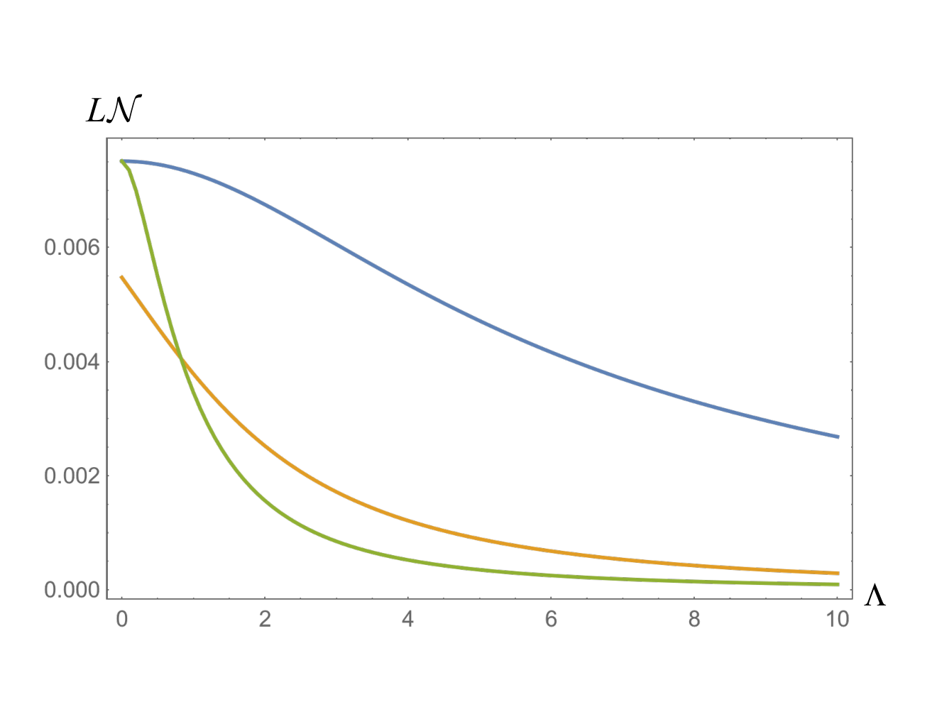
\displaystyle L{\cal N}(\nu)=\frac{1}{\pi}\int_{0}^{\infty}dp\,p^{2}L{\cal N}(p,\,\nu)\,.

(3.48)

The result is plotted in Figure 5. We find that the qualitative features are the same as the result of entanglement entropy.

4 Summary and discussion

We have studied the effect of a bubble wall on the entanglement entropy of a free massive scalar field between two causally disconnected open charts in de Sitter space. We assume there is a delta-functional wall between them parameterized by our wall parameter $\Lambda$ . This may be regarded as a model describing the pair creation of identical bubble universes separated by a bubble wall. To analyze the system, we first derived the Euclidean vacuum mode functions of the scalar field in the presence of the wall in the coordinates that respect the open charts. We then gave the Bogoliubov transformation between the Euclidean vacuum and the open chart vacua that makes the reduced density matrix diagonal. We derived the reduced density matrix in one of the open charts ( $R$ space) after tracing out the other ( $L$ space). We then computed the entanglement entropy of the scalar field by using the reduced density matrix and compared the result with the case of no bubble wall. We found that larger values of parameter $\Lambda$ correspond to less entanglement. We also computed a different measure of entanglement called logarithmic negativity. The qualitative features were found to be the same as the result of entanglement entropy.

In the limit of small entanglement entropy the BD quantum state approaches a product of ground state wavefunctions for each of the charts. Our results thus show that for large $\Lambda$ the dynamics of bubble formation select this product state and ensure its stability under evolution. These are the features identified in the literature⁵⁵ 5 See for example [35, 36, 37, 38] and also [39], section IV-D, for a nice review. to correspond to the selection of special “pointer states” via the decoherence process. Our results thus may be regarded as evidence of decoherence of bubble universes from (and by) each other.

We also note that in discussions of the black hole firewall problem [33, 34] it is argued that the absence of entanglement implies the existence of a firewall. We are intrigued by a certain parallel, in a kind of reverse engineered way, with our results: We show a particular example of how the presence of a wall can reduce entanglement.

Acknowledgments

This work was supported in part by the MEXT KAKENHI Nos. 15H05888 and 15K21733. SK was supported by IKERBASQUE, the Basque Foundation for Science and the Basque Government (IT-979-16), and Spanish Ministry MINECO (FPA2015-64041-C2-1P). AA was supported by a grant from UC Davis, and thanks A. Arrasmith for helpful conversations.

Appendix A Supercurvature mode

On the de Sitter background, there exists a supercurvature mode in the open chart if the mass-squared is in the range $0<m^{2}/H^{2}<2$ [3]. The supercurvature mode has an imaginary eigenvalue, $p=ik$ where $0<k<1$ . Therefore this may be regarded as a bound-state mode in the spectrum.

The role of supercurvature modes in the quantum entanglement is not known. In [4], it is conjectured that they do not contribute to the entanglement. Here we consider the effect of the presence of a bubble wall on the supercurvature mode by focusing on the simplest case of $m^{2}/H^{2}=2$ , ie, the conformal scalar case. In this case, if there is no wall, there is no supercurvature mode. We see below that a supercurvature mode appears when there is a wall.

Let us first write down the equation for the mode function $\chi_{p}(t_{C})$ in region $C$ ,

\displaystyle\left[\frac{d^{2}}{dt_{C}^{2}}+\frac{da(t_{C})}{a(t_{C})dt_{C}}\frac{d}{dt_{C}}+2-M^{2}(t_{C})+\frac{p^{2}}{H^{2}a^{2}(t_{C})}\right]\chi_{p}=0\,,

(A.1)

where $a(t_{C})=H^{-1}\cos t_{C}$ and

\displaystyle M^{2}=\frac{m^{2}-\Lambda\delta(t_{C})}{H^{2}}\,.

(A.2)

By using the conformal coordinate $d\xi=dt_{C}/a(t_{C})$ , we have $a=(H\cosh\xi)^{-1}$ and Eq. (A.1) is re-expressed as

\displaystyle\left[-\frac{d^{2}}{d\xi^{2}}+\frac{M^{2}-2}{\cosh^{2}\xi}-p^{2}\right]\chi_{p}=0\,.

(A.3)

We set $p^{2}=-k^{2}$ $(k>0)$ , since we consider a supercurvature mode. For $M^{2}=2$ , Eq. (A.3) gives the solution,

\displaystyle\chi_{k}\propto e^{\pm k\xi}\qquad\mbox{for}\quad\xi\neq 0\,.

(A.4)

For either sign, the solution is singular at $\xi\to\mp\infty$ if there were no wall. However, the presence of a wall allows the solution to be

\displaystyle\chi_{k}\propto\left\{\begin{array}[]{ll}e^{-k\xi}&\mbox{for}~\xi>0\,,\\ e^{k\xi}&\mbox{for}~\xi<0\,.\end{array}\right.

The matching condition at $\xi=0$ gives

\displaystyle\left[-\frac{d}{d\xi}\chi_{p}\right]^{+}_{-}=\frac{\Lambda}{H^{2}}\chi_{p}\,,

(A.7)

which can be readily solved to obtain

\displaystyle k=\frac{\Lambda}{2H^{2}}\,.

(A.8)

Thus the supercurvature mode exists for any value of $\Lambda>0$ , and the eigenvalue $k$ can be arbitrarily large unlike the case of the pure de Sitter background.

To complete the analysis, let us compute the normalization factor of the supercurvature mode. Setting $\chi_{k}=N_{k}^{-1}e^{\pm k\xi}$ for $\xi\lessgtr 0$ , we have

\displaystyle 1=\int_{-\infty}^{\infty}d\xi|\chi_{k}|^{2}=\frac{2}{N_{k}^{2}}\int_{0}^{\infty}d\xi e^{-2k\xi}=\frac{1}{N_{k}^{2}k}\,.

(A.9)

Thus we obtain a very simple result,

\displaystyle N_{k}=\frac{1}{\sqrt{k}}\,.

(A.10)

Thus the larger the eigenvalue $k$ , the smaller the normalization factor becomes, implying that its contribution to the spectrum of the vacuum fluctuations in each open chart becomes more and more important [31].

Appendix B Transformation formulas

	$\displaystyle F\left(\alpha,\beta,\gamma;z\right)$	$\displaystyle=$	$\displaystyle\frac{\Gamma(\gamma)\Gamma(\alpha+\beta-\gamma)}{\Gamma(\alpha)\Gamma(\beta)}\left(1-z\right)^{\gamma-\alpha-\beta}F\left(\gamma-\alpha\,,\gamma-\beta\,,\gamma-\alpha-\beta+1\,;1-z\right)$		(B.1)
			$\displaystyle+\frac{\Gamma(\gamma)\Gamma(\gamma-\alpha+\beta)}{\Gamma(\gamma-\alpha)\Gamma(\gamma-\beta)}F\left(\alpha\,,\beta\,,\alpha+\beta-\gamma+1\,;1-z\right)\,,$		(B.1)

and

\displaystyle F\left(\alpha,\beta,\gamma;z\right)=\left(1-z\right)^{\gamma-\alpha-\beta}F\left(\gamma-\alpha\,,\gamma-\beta\,,\gamma\,;z\right)\,.

(B.2)

Appendix C Bogoliubov coefficients

From Eq. (2.16), the relation between the operators $a_{I}$ and $b_{J}$ is given by

\displaystyle b_{J}=a_{I}\left(M\right)^{I}{}_{J}\,,\qquad b_{J}=\left(b_{q}\,,b_{q}^{\dagger}\right)\,,\qquad a_{I}=\left(a_{\sigma}\,,a_{\sigma}^{\dagger}\right)\,,

(C.1)

where the capital indices $\left(I\,,J\right)$ run from $1$ to $4$ , the subscripts $q,\sigma=\left(R\,,L\right)$ and $M$ is a $4\times 4$ matrix

\displaystyle M^{I}{}_{J}=\left(\begin{array}[]{cc}\alpha^{\sigma}{}_{q}&\beta^{\sigma}{}_{q}\\ \beta^{\sigma*}{}_{\!\!\!q}&\alpha^{\sigma*}{}_{\!\!\!q}\\ \end{array}\right)\,,

and $\alpha$ and $\beta$ are $2\times 2$ matrices and consist of $f_{p}$ and $g_{p}$ in Eq. (3.36) such as

\displaystyle\alpha^{\sigma}{}_{q}=\frac{\tilde{N}_{p}}{N_{w}}\left(\begin{array}[]{cc}1&f_{p}\\ f_{p}&1\\ \end{array}\right)\,,\qquad\beta^{\sigma}{}_{q}=\frac{\tilde{N}_{p}}{N_{w}}\left(\begin{array}[]{cc}0&g_{p}\\ g_{p}&0\\ \end{array}\right)\,.

The relation (C.1) is rewritten as

\displaystyle a_{J}=b_{I}\left(M^{-1}\right)^{I}{}_{J}\,,\qquad\left(M^{-1}\right)^{I}{}_{J}=\left(\begin{array}[]{ll}\xi_{q\sigma}&\delta_{q\sigma}\\ \delta_{q\sigma}^{*}&\xi_{q\sigma}^{*}\\ \end{array}\right)\,,\qquad\left\{\begin{array}[]{l}\xi=\left(\alpha-\beta\,\alpha^{*\,-1}\beta^{*}\right)^{-1}\,,\\ \delta=-\alpha^{-1}\beta\,\xi^{*}\,.\end{array}\right.

By using Eq. (C), we find the above matrices $\xi$ and $\delta$ are expressed respectively as

	$\displaystyle\xi$	$\displaystyle=$	$\displaystyle\frac{N_{w}}{\tilde{N}_{p}}\frac{1}{E}\left(\begin{array}[]{cc}1-\frac{\|g_{p}\|^{2}}{1-f_{p}^{2}}&-f_{p}-\frac{f_{p}^{}\|g_{p}\|^{2}}{1-f_{p}^{2}}\\ -f_{p}-\frac{f_{p}^{}\|g_{p}\|^{2}}{1-f_{p}^{2}}&1-\frac{\|g_{p}\|^{2}}{1-f_{p}^{2}}\\ \end{array}\right)\,,$
	$\displaystyle\delta$	$\displaystyle=$	$\displaystyle\frac{N_{w}}{\tilde{N}_{p}}\frac{1}{E^{}}\frac{g_{p}}{1-f_{p}^{2}}\left(\begin{array}[]{cc}f_{p}+f_{p}^{}&-1-\|f_{p}\|^{2}+\|g_{p}\|^{2}\\ -1-\|f_{p}\|^{2}+\|g_{p}\|^{2}&f_{p}+f_{p}^{*}\\ \end{array}\right)\,.$

If we apply $a_{\sigma}$ to Eq. (2.17), then we have

\displaystyle 0=a_{\sigma}\,|0\rangle_{\rm BD}\Longrightarrow m_{ij}=-\left(\delta^{*}\xi^{-1}\right)_{ij}\,,

(C.21)

and $m_{ij}$ is found to be

\displaystyle m_{ij}=\left(\begin{array}[]{cc}\omega&\zeta\\ \zeta&\omega\\ \end{array}\right)\,,

where $\omega$ and $\zeta$ are given in Eqs. (3.37) and (3.38).

References

[1] A. Aspect, P. Grangier and G. Roger, Phys. Rev. Lett. 47, 460 (1981).
[2] A. Aspect, J. Dalibard and G. Roger, Phys. Rev. Lett. 49, 1804 (1982).
[3] M. Sasaki, T. Tanaka and K. Yamamoto, Phys. Rev. D 51, 2979 (1995) [gr-qc/9412025].
[4] J. Maldacena and G. L. Pimentel, JHEP 1302, 038 (2013) [arXiv:1210.7244 [hep-th]].
[5] S. Kanno, J. Murugan, J. P. Shock and J. Soda, JHEP 1407, 072 (2014) [arXiv:1404.6815 [hep-th]].
[6] N. Iizuka, T. Noumi and N. Ogawa, Nucl. Phys. B 910, 23 (2016) [arXiv:1404.7487 [hep-th]].
[7] S. Kanno, M. Sasaki and T. Tanaka, JHEP 1703, 068 (2017) [arXiv:1612.08954 [hep-th]].
[8] S. Choudhury and S. Panda, Eur. Phys. J. C 78, no. 1, 52 (2018) [arXiv:1708.02265 [hep-th]].
[9] S. Choudhury and S. Panda, arXiv:1712.08299 [hep-th].
[10] S. Kanno, JCAP 1407, 029 (2014) [arXiv:1405.7793 [hep-th]].
[11] F. V. Dimitrakopoulos, L. Kabir, B. Mosk, M. Parikh and J. P. van der Schaar, JHEP 1506, 095 (2015) [arXiv:1502.00113 [hep-th]].
[12] S. Ryu and T. Takayanagi, Phys. Rev. Lett. 96, 181602 (2006) [hep-th/0603001].
[13] V. E. Hubeny, M. Rangamani and T. Takayanagi, JHEP 0707, 062 (2007) [arXiv:0705.0016 [hep-th]].
[14] D. Campo and R. Parentani, Phys. Rev. D 74, 025001 (2006) [astro-ph/0505376].
[15] D. Campo and R. Parentani, Braz. J. Phys. 35, 1074 (2005) [astro-ph/0510445].
[16] J. Maldacena, Fortsch. Phys. 64, 10 (2016) [arXiv:1508.01082 [hep-th]].
[17] J. Martin and V. Vennin, Phys. Rev. A 93, no. 6, 062117 (2016) [arXiv:1605.02944 [quant-ph]].
[18] S. Choudhury, S. Panda and R. Singh, Eur. Phys. J. C 77, no. 2, 60 (2017) [arXiv:1607.00237 [hep-th]].
[19] S. Kanno and J. Soda, Phys. Rev. D 96, no. 8, 083501 (2017) [arXiv:1705.06199 [hep-th]].
[20] J. Martin and V. Vennin, Phys. Rev. D 96, no. 6, 063501 (2017) [arXiv:1706.05001 [astro-ph.CO]].
[21] Y. Nambu, Phys. Rev. D 78, 044023 (2008) [arXiv:0805.1471 [gr-qc]].
[22] S. Kanno, J. P. Shock and J. Soda, JCAP 1503, no. 03, 015 (2015) [arXiv:1412.2838 [hep-th]].
[23] A. Matsumura and Y. Nambu, arXiv:1707.08414 [gr-qc].
[24] J. Martin and V. Vennin, Phys. Rev. D 93, no. 2, 023505 (2016) [arXiv:1510.04038 [astro-ph.CO]].
[25] S. Kanno, J. P. Shock and J. Soda, Phys. Rev. D 94, no. 12, 125014 (2016) [arXiv:1608.02853 [hep-th]].
[26] A. Albrecht, N. Bolis and R. Holman, JHEP 1411, 093 (2014) [arXiv:1408.6859 [hep-th]].
[27] S. Kanno, EPL 111, no. 6, 60007 (2015) [arXiv:1507.04877 [hep-th]].
[28] S. Kanno, Phys. Lett. B 751, 316 (2015) [arXiv:1506.07808 [hep-th]].
[29] H. Collins and T. Vardanyan, JCAP 1611, no. 11, 059 (2016) [arXiv:1601.05415 [hep-th]].
[30] N. Bolis, A. Albrecht and R. Holman, JCAP 1612, no. 12, 011 (2016) Erratum: [JCAP 1708, no. 08, E01 (2017)] [arXiv:1605.01008 [hep-th]].
[31] K. Yamamoto, M. Sasaki and T. Tanaka, Phys. Rev. D 54, 5031 (1996) [astro-ph/9605103].
[32] R. Horodecki, P. Horodecki, M. Horodecki and K. Horodecki, Rev. Mod. Phys. 81, 865 (2009) [quant-ph/0702225].
[33] S. L. Braunstein, S. Pirandola and K. Życzkowski, Phys. Rev. Lett. 110, no. 10, 101301 (2013) [arXiv:0907.1190 [quant-ph]].
[34] A. Almheiri, D. Marolf, J. Polchinski and J. Sully, JHEP 1302, 062 (2013) [arXiv:1207.3123 [hep-th]].
[35] W. H. Zurek, Phys. Rev. D 24, 1516 (1981).
[36] W. H. Zurek, S. Habib and J. P. Paz, Phys. Rev. Lett. 70, 1187 (1993).
[37] W. H. Zurek, Prog. Theor. Phys. 89, 281 (1993).
[38] J. R. Anglin and W. H. Zurek, Phys. Rev. D 53, 7327 (1996) [quant-ph/9510021].
[39] W. H. Zurek, Rev. Mod. Phys. 75, 715 (2003).