Deep learning algorithm for data-driven simulation of noisy dynamical system

The Long Short-Term Memory network was introduced to consider a delay-time process, where the state of a system at time $t$ is affected by a past event at $t-\tau$ [24]. The basic equations of LSTM unit proposed by [25] consist of a set of nonlinear transformations of an input variable $z\in\mathbb{R}^{m}$;

in which $\bm{\varphi}_{S}$ and $\bm{\varphi}_{T}$, respectively, denote the sigmoid and hyperbolic tangent functions, $\mathcal{L}^{n}$ is a linear transformation operator, $N_{c}$ is the number of the LSTM units, $s_{t}$ and $h_{t}$ represent, respectively, the internal state and the output of the LSTM network, and $\bm{a}\odot\bm{b}$ denotes a component-wise multiplication of two vectors. The linear transformation operator is defined as

where $\bm{W}\in\mathbb{R}^{n\times m}$ for $\bm{x}\in\mathbb{R}^{m}$ and $\bm{B}\in\mathbb{R}^{n}$ denote a weight matrix and a bias vector, respectively.

Figure 1 (a) shows a sketch of one LSTM unit. The sigmoid function, which varies between zero and one, is employed in the gate functions. An LSTM network learns from the data when to close ($\varphi_{S}(x)=0$) or open ($\varphi_{S}(x)=1$) each gates to control information flow into and out of the LSTM units. Equation 4 shows that, when the input gate is closed, $\bm{G}_{i}=0$, and the forget gate is inactive, $\bm{G}_{f}=1$, the internal state of the LSTM unit is conserved. Hence, the information stored in an LSTM unit can be carried for a long time period.

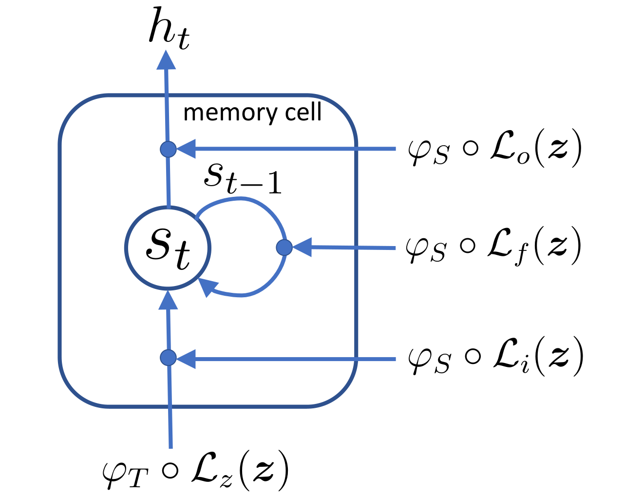
Figure 1 (b) outlines a typical LSTM network architecture to make a prediction of a target variable at the next time step, $\bm{y}_{t+1}$, from an input variable at the current time, $\bm{x}_{t}$. An LSTM network is “fully connected”, meaning that the output of LSTM in the previous time step, $\bm{h}_{t-1}$, is used as an input to the LSTM itself. The updated internal state, $\bm{s}_{t}$, is carried to the next step (dashed arrow). There are two additional feedforward neural networks, $\mathcal{F}_{in}$ and $\mathcal{F}_{out}$, before and after the LSTM, which connects the input variable to the LSTM network and performs a nonlinear transformation of the output of the LSTM network to compute the target variable.

LSTM can be understood as a nonlinear state-space model. Observe that, from the anti-symmetry of $\varphi_{S}$, $\bm{G}_{f}(\bm{z})=1-\bm{G}_{f}(-\bm{z})$, and the last term in (4) depends only on $\bm{z}$, $\bm{G}_{i}(\bm{z})\odot\left(\bm{\varphi}_{T}\circ\mathcal{L}^{N_{c}}_{z}(\bm{z})\right)=g^{*}(\bm{z})$. Then, the update rule of $\bm{s}$ in (4) can be written as

in which $\delta t$ is the sampling interval of the data, and $0<f(\cdot)<\delta t^{-1}$ and $|g(\cdot)|<\delta t^{-1}$ are some unknown functions. The time evolution of the internal state is essentially a forward Euler scheme for a system of relaxation processes,

The artificial neural network operating on $\bm{x}_{t}$ and $\bm{h}_{t-1}$ provides nonlinear estimations of the relaxation ($f$) and forcing ($g$) functions. Once LSTM computes the internal phase dynamics by solving (7), another artificial neural network, $\mathcal{F}_{out}$ in figure 1 (b), is used for a nonlinear projection of the internal dynamics $\bm{s}_{t}$ onto the phase space of the target variable, $\bm{y}_{t+1}$.

It is important to note that the time evolution of $\bm{s}$ is given as a set of relaxation equations. For a simulation by LSTM, we need to specify the initial conditions, i.e., $\bm{s}_{0}$ and $\bm{h}_{0}$. It is challenging, if not impossible, to find a correct initial condition for the data-driven simulation. But, equation (7) suggests that the effects of the initial conditions will eventually vanish after some spin-up time and the system becomes stationary.

Here, we consider noisy time series data from a dynamical system. Let $\hat{y}(t)$ be a noisy observation of a dynamical system,

in which $\bm{u}$ is an exogenous forcing. For simplicity, we consider a univariate dynamical system, but the modeling framework can be easily extended to a multivariate time series. In general, the ground truth, $y(t)$, is not accessible and we observe only a discrete, corrupted time series,

where $\epsilon_{t}$ is a white noise. Hereafter, a subscript $t$ indicates a projection onto a discrete space, e.g., $y_{t+n}=\int y(s)\delta(t+n\delta t-s)ds$, and a sampling interval is denoted by $\delta t$. Here, we are interested in a prediction of the probability distribution of $\hat{y}$, $p(\hat{y}_{t+1}|\widehat{\bm{Y}}_{0:t},\bm{U}_{0:t})$, given the past trajectories of the observation, $\widehat{\bm{Y}}_{0:t}=(\hat{y}_{0},\cdots,\hat{y}_{t})$, and the exogenous forcing, $\bm{U}_{0:t}=(\bm{u}_{0},\cdots,\bm{u}_{t})$.

Note that, in LSTM, the probability distribution of $\hat{y}$ can be represented as a Markov process, i.e., $p(\hat{y}_{t+1}|\widehat{\bm{Y}}_{0:t},\bm{U}_{0:t})=p(\hat{y}_{t+1}|\bm{h}_{t})$. From the LSTM equations (1–5), we can summarize the overall algorithm in the following three steps,

in which $\bm{x}_{t}=(\hat{y}_{t},\bm{u}_{t})$, $\Psi_{h}=\bm{s}_{t}\odot\bm{G}_{o}$, and $\Psi_{y}$ is a feed forward neural network, shown as $\mathcal{F}_{out}$ in figure 1 (b). It is clear that, once $\bm{h}_{t}$ is given, $\hat{y}_{t+1}$ is obtained independently from the past trajectory. In other words, the past information is stored in the internal dynamical system of LSTM and $\hat{y}_{t+1}$ becomes conditionally independent from $\widehat{\bm{Y}}_{0:t}$ and $\bm{U}_{0:t}$. Hence, we first consider the last part of the LSTM of estimating the probability distribution of a target variable, $\hat{y}_{t+1}$, given an input vector $\bm{h}_{t}$, $p(\hat{y}_{t+1}|\bm{h}_{t})$.

Here, we use a notation $p(y|\bm{x})$, instead of $p(\hat{y}_{t+1}|\bm{h}_{t})$, for simplicity. Suppose there is a mapping $\mathcal{C}:\mathbb{R}\rightarrow\mathbb{N}_{+}$, such that

Here, $\bm{\alpha}\in\mathbb{R}^{K+1}$ is a set of ordered real numbers; $\alpha_{1}<\alpha_{2}<\cdots<\alpha_{K+1}$. Then, we can define a discrete probability as

The discrete probability, $P(k|\bm{x})$, is a numerical discretization of the continuous probability distribution, $p(y|\bm{x})$. In the computer science literature, $P(k|\bm{x})$ is called the “class probability”, as it indicates the probability of $y$ belonging to the $k$-th class, or interval, $\mathcal{I}_{k}=(\alpha_{k},\alpha_{k+1})$. After the discretization, the original problem of estimating a continuous probability function is converted into a multi-label classification problem.

Suppose there is a data set $\bm{D}=\{(y_{i},\bm{x}_{i});i=1,\cdots,N\}$. Then, we can create a new data set by applying $\mathcal{C}$, such that $\bm{D}_{C}=\{(c_{i},\bm{x}_{i});c_{i}=\mathcal{C}(y_{i})~\text{and}~i=1,\cdots,N\}$. The likelihood function for $\bm{D}_{C}$ is the generalized Bernoulli distribution, or multinoulli distribution, [33]

Here, $\bm{X}=(\bm{x}_{1},\cdots,\bm{x}_{n})$, $\bm{\theta}$ is the parameters of the artificial neural network, and $\delta_{ij}$ is the Kronecker delta function. The discrete probability, $P(k|\bm{x})$ is modeled by an artificial neural network, $\bm{\Psi}(\bm{x};\bm{\theta})$, with a softmax function. The output of the artificial neural network, $\bm{\Psi}(\bm{x};\bm{\theta})$, is a vector of length $K$, and the softmax function is defined as,

By definition, the softmax function is $P_{k}>0$ and $\sum_{k}P_{k}=1$.

The parameters of the artificial neural network, $\bm{\theta}$, are estimated by a maximum likelihood method, or by minimizing a negative log likelihood. Let $l(\bm{\theta})$ be a negative log likelihood function,

Here, $P_{k}^{n}(\bm{\Psi})$ is a short notation of $P_{k}(\bm{\Psi}(\bm{x}_{n};\bm{\theta}))$. A maximum likelihood estimator is

in which $N_{w}$ is the total number of parameters in $\Psi(\bm{x};\bm{\theta})$. In deep learning, the minimization problem is usually solved by a gradient descent method,

where the superscript $k$ is the number of iteration and $\eta$ is a learning rate. The gradient of $l(\bm{\theta})$ with respect to the output vector of $\Psi(\bm{x};\bm{\theta})$ is

and the full gradient is simply

The gradient of the output vector with respect to the parameters, $\partial\Psi_{i}/\partial\bm{\theta}$, in (21) can be easily computed by a back-propagation algorithm [23].

The negative log likelihood function (17) corresponds to the cross entropy between probability distributions from the data and the model. This kind of cross-entropy minimization is one of the most widely used methods to train a deep neural network for classification. However, the cross-entropy minimization does not explicitly guarantee the smoothness of the estimated distribution. In (18), the multinoulli loss function depends only on $\bm{P}(\bm{\Psi})$ of a correct label, $\delta_{c_{n}k}$. As a result, equation (20) indicates that, in the gradient decent steps (19), every $P_{i}(\bm{\Psi})$ except for the one for the correct label, $P_{c_{n}}(\bm{\Psi})$, is penalized in the same way. So, there is no explicit way to guarantee smoothness of the estimated distribution. In the conventional classification tasks, a geometric proximity between the classes is not relevant. In the present study, however, the softmax function is used as a discrete approximation to a probability density function, which requires a smoothness in $\bm{P}(\bm{\Psi})$.

To impose the smoothness constraint, we propose a penalized maximum likelihood method, inspired by a non-parametric density estimation problem [40]. The penalized maximum likelihood estimator is computed by adding a regularization to the standard cross-entropy loss function;

in which $\lambda$ is a penalty parameter, $\bm{D}$ is a diagonal matrix, $D_{ij}=\Delta_{i+1}\delta_{ij}$ for $i=1,\cdots,K-2$, and $\Delta_{i}=|\mathcal{I}_{i}|=\alpha_{i+1}-\alpha_{i}$. The Laplacian matrix $\bm{L}\in\mathbb{R}^{K-2,K}$ is

Here,

and

Suppose there is a smooth function, $g(y)$, such that

where $\alpha_{i+1/2}=0.5(\alpha_{i}+\alpha_{i+1})$. The regularization in (22) corresponds to

This regularized cross-entropy (RCE) aims to smooth out the estimated distribution by penalizing local minima or maxima.

Let $l^{*}(\bm{\theta})$ denote RCE (22), the gradient of $l^{*}(\bm{\theta})$ with respect to $\bm{\Psi}(\bm{x}^{n};\bm{\theta})$ is

in which $\bm{M}=\bm{L}^{T}\bm{D}\bm{L}$ and $\bm{M}_{i,\cdot}\bm{P}=\sum_{j}M_{ij}P_{j}$. Comparing to (20), the additional computational cost to consider the smoothness is only the maxtrix-vector multiplications in the curly bracket in (27).

Extending the RCE minimization to a time series data is straightforward. Suppose we have a data set, which consist of $N$ time series with length $T$; $\mathcal{D}_{y}=\{(\bm{\hat{y}}^{n},\bm{u}^{n});\bm{\hat{y}}^{n}\in\mathbb{R}^{T}~\text{and}~\bm{u}^{n}\in\mathbb{R}^{T\times m}~\text{for}~n=1,\cdots,N\}$. By applying $\mathcal{C}$, the data set can be converted to $\mathcal{D}_{c}=\{(\bm{c}^{n},\bm{\hat{y}}^{n},\bm{u}^{n});\bm{c}^{n}=\mathcal{C}(\bm{\hat{y}}^{n}),\bm{\hat{y}}^{n}\in\mathbb{R}^{T},~\text{and}~\bm{u}^{n}\in\mathbb{R}^{T\times m}~\text{for}~n=1,\cdots,N\}$. The data likelihood function for $\mathcal{D}_{c}$ is given as

where $\bm{x}^{n}_{l}=(\hat{y}^{n}_{l},\bm{u}^{n}_{l})$. The regularized cross-entropy for LSTM is

and,

in which $\bm{P}^{n}_{l+1}=\bm{\Psi}_{y}(\bm{h}^{n}_{l})$. The regularized cross-entropy minimization problem for LSTM can be solved by the standard back-propagation through time algorithm (BPTT) [23]. In BPTT, the temporal structure of error is propagated backward in time, e.g.,

It is explicitly shown that the gradient of the loss function at $t$ is linked to the loss function at the next time step, $l^{*}_{t+1}$. For more details, see [41].

One of the major interests in time series modeling is to make a multiple-step forecast of the state of the system conditioned on the past observations. For a noisy dynamical system with an exogenous forcing, (8 – 9), a multi-step forecast is to compute the future probability distribution, $p(\hat{y}_{t+n}|\widehat{\bm{Y}}_{0:t},\bm{U}_{0:t+n-1})$ for $n>1$, given the past trajectories, $(\widehat{\bm{Y}}_{0:t},\bm{U}_{0:t})$, and a future forcing scenario, $\bm{U}_{t+1:t+n-1}$. In other words, we are interested in computing a temporal evolution of the probability distribution for a given forcing scenario.

A multiple-step forecast can be achieved by successively applying the deterministic transformations in (10 – 12). Suppose the data is given up to time $t$, i.e., we have $(\widehat{\bm{Y}}_{0:t},\bm{U}_{0:t})$. The probability distribution at $t+1$ is computed by a deterministic update,

Again, from the state-space model argument in sections 2.1 and 2.2, we have $p(\hat{y}_{t+1}|\widehat{\bm{Y}}_{0:t},\bm{U}_{0:t})=p(\hat{y}_{t+1}|\bm{h}_{t})$. In the next time step at $t+2$, the internal state is updated as,

Because the observation is available only up to $\hat{y}_{t}$, $\hat{y}_{t+1}$ becomes a random variable, of which distribution is computed in (32). Hence, $\bm{s}_{t+1}$ becomes a random variable and the probability distribution of $\bm{s}_{t+1}$ is fully determined by $(\bm{h}_{t},\bm{s}_{t},\bm{u}_{t+1})$, i.e., $p(\bm{s}_{t+1}|\bm{s}_{t},\bm{h}_{t},\bm{u}_{t+1})$. Similarly, the probability distribution of $\bm{h}_{t+1}$ is given as $p(\bm{h}_{t+1}|\bm{s}_{t+1},\bm{h}_{t},\bm{u}_{t+1})$. Finally, the probability distribution of $\hat{y}$ at $t+2$, $p(\hat{y}_{t+2}|\widehat{\bm{Y}}_{0:t},\bm{U}_{0:t+1})$, is

Here, a product rule is used,

From a recurrent relation, the multiple-step forecast is

in which $\bm{H}_{t}=(\bm{h}_{t},\bm{s}_{t})$. Equation (34) is computed by using (10 – 11) as an initial condition. In practice, directly computing the probability distribution of the LSTM states, $p(\bm{H}_{t+1}|\bm{H}_{t})$, is intractable because of the high dimensionality, $\bm{H}\in\mathbb{R}^{2N_{c}}$. Here, we outline a Monte Carlo simulation to approximate the high-dimensional integration in (34) in Algorithm 1.

First, we consider the Ornstein–Uhlenbeck process, which is represented by the following stochastic differential equation,

in which $\tau$ is a relaxation timescale and $W$ is the Weiner process. The Ornstein–Uhlenbeck process has a closed form solution;

The parameters used in this example are, $\tau=1$, $\xi=\sqrt{2}$, and $\delta t=0.1$. Note that, in this example, we do not distinguish the noisy observation, $\hat{y}_{t}$, from the ground truth, $y_{t}$, because $y_{t}$ itself is a stochastic process.

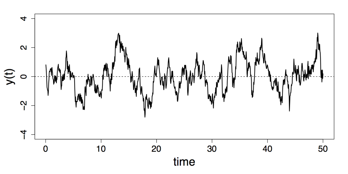
Figure 2 shows a sample trajectory of the Ornstein-Uhlenbeck process. A simulation is performed for $4\times 10^{5}\delta t$ to generate a training set and for another $2\times 10^{3}\delta t$ to make a data set for model validation. The initial learning rate is $\eta_{0}=10^{-3}$ and it is decreased with the number of iteration, $k$, as $\eta_{k}=\eta_{0}/(1+10^{-3}k)$. At each iteration, 20 sample trajectories with identical length, $T=100$, are used as a minibatch. The starting point of each sample trajectory is randomly selected from the training data set, $t_{0}\in[1,4\times 10^{5}-T]\delta t$. The size of the bins to discretize the probability distribution is uniform, i.e., $\Delta_{1}=\cdots=\Delta_{K}=\delta y$.

Figure 3 demonstrates an example of the DE-LSTM simulation. In this example, the discretization interval is $\delta y=0.04$. Here, we consider the next-step prediction problem, in which DE-LSTM is used to compute $p(dy_{t}|y_{t})$. Note that the Ornstein-Uhlenbeck process is a Markov process, $p(dy_{t}|\bm{Y}_{0:t})=p(dy_{t}|y_{t})$. The prediction is made as, $E[y_{t+1}|y_{t}]=y_{t}+E[dy_{t}|y_{t}]$. The expectation and higher-order moments are easily computed by a numerical integration. For example,

in which $\alpha_{i+1/2}=0.5(\alpha_{i}+\alpha_{i+1})$. Compared to the deterministic LSTM used for regression, DE-LSTM directly estimates the probability distribution, which provides rich information about the uncertainty in the prediction. For example, as shown in figure 3 (a), DE-LSTM can provide the prediction together with uncertainty.

The estimated probability distribution by DE-LSTM is shown in figure 3 (b). The probability distribution is computed at the vertical dashed line in figure 3 (a). As expected, when the regularization is not used, i.e., $\lambda=0$, the estimated distribution is bumpy. For $\lambda=0.1$, it is shown that the estimated distribution becomes smooth.

For a quantitative comparison, a normalized root mean-square error (NRMSE) of $E[y_{t+1}|y_{t}]$ is computed as

in which $\langle\cdot\rangle$ denotes an ensemble average, and $p_{T}$ and $p_{L}$ are the true and DE-LSTM probability distributions, respectively. The normalized root mean-square error compares the prediction error between DE-LSTM and a zeroth order prediction, which assumes $y_{t+1}=y_{t}$. Similarly, NRMSE of the standard deviation is defined as

Tables 1 and 2 show $e_{\mu}$ and $e_{sd}$, respectively.

In Table 1, it is shown that DE-LSTM trained with RCE, i.e., $\lambda>0$, makes a better prediction of the expectation. As $\lambda$ is increased, $e_{\mu}$ reduces at first, then above a threshold $e_{\mu}$ starts to increase. Such dependence on the penalty parameter is typical for a penalized maximum likelihood method. It should be noted that $e_{\mu}$ is not sensitive to the changes in $\lambda$. For example, for $\delta y=0.04$, the difference between the maximum and minimum $e_{\mu}$ is only 0.011, when there is a fiftyfold increase in $\lambda$; $\lambda=0.01$ – 0.5.

It is observed that, when RCE is used, the grid resolution, $\delta y$, does not have a noticeable effect in the estimation of the expectation. Except for $\lambda=0$, $e_{\mu}$ for $\delta y=0.08$ is very close to that of $\delta y=0.04$. On the other hand, $e_{sd}$ in Table 2 clearly shows the impact of $\delta y$ on the estimation of the probability distribution. When a fine resolution ($\delta y=0.04$) is used, not only $e_{sd}$ is smaller than that of $\delta y=0.08$, but also the sensitivity of $e_{sd}$ to $\lambda$ is much smaller. As $\lambda$ changes from 0.001 to 0.1, $e_{sd}$ for $\delta y=0.08$ increases from 0.0039 to 0.022, while, for $\delta y=0.04$, $e_{sd}$ changes only from 0.0030 to 0.0082.

While $e_{\mu}$ and $e_{sd}$ provide useful information on the behaviors of DE-LSTM, those metrics only compare the first and second moments of the probability distribution. To make a more thorough comparison of the estimated probability distribution, the Kullback–Leibler divergence is computed. Here, the Kullback–Leibler divergence is defined as

Here, $P_{i}$ is the $i$-th output of DE-LSTM and $Q_{i}$ is the true probability distribution,

References

- [1] S. L. Brunton, J. L. Proctor, J. N. Kutz, Discovering governing equations from data by sparse identification of nonlinear dynamical systems, Proc. Natl. Acad. Sci. 113 (2016) 3932 – 3937.
- [2] H. Jaeger, H. Haas, Harnessing nonlinearity: Predicting chaotic systems and saving energy in wireless communications, Science 304 (2004) 78–80.
- [3] W.-X. Wang, Y.-C. Lai, C. Grebogi, Data based identification and prediction of nonlinear and complex dynamical systems, Phys. Reports 644 (2016) 1–76.
- [4] K. Ikeda, H. Daido, O. Akimoto, Optical turbulence: Chaotic behavior of transmitted light from a ring cavity, Phys. Rev. Lett. 45 (1980) 709–712.
- [5] H. Ma, S. Leng, C. Tao, X. Ying, J. Kurths, Y.-C. Lai, W. Lin, Detection of time delays and directional interactions based on time series from complex dynamical systems, Phys. Rev. E 96 (2017) 012221.
- [6] M. Mackey, L. Glass, Oscillation and chaos in physiological control systems, Science 197 (1977) 287–289.
- [7] S. Yanchuk, G. Giacomelli, Spatio-temporal phenomena in complex systems with time delays, J. Phys. A.:Math. Theor. 50 (2017) 103001.
- [8] G. E. P. Box, G. M. Jenkins, G. C. Reinsel, Time series analysis, John Wiley & Sons, Inc., 2008.
- [9] J. Durbin, S. J. Koopman, Time series analysis by state space model, Oxford University Press, 2012.
- [10] A. C. Harvey, Forecasting, structural time series models and the Kalman filter, Cambridge university press, 1990.
- [11] E. A. Wan, R. V. D. Merwe, The unscented kalman filter for nonlinear estimation, in: Proceedings of the IEEE 2000 Adaptive Systems for Signal Processing, Communications, and Control Symposium, 2000, pp. 153–158.
- [12] G. Evensen, The ensemble Kalman filter: theoretical formulation and practical implementation, Ocean Dyn. 53 (2003) 343 – 367.
- [13] R. van der Merwe, A. Doucet, N. de Freitas, E. A. Wan, The unscented particle filter, in: Advances in Neural Information Processing Systems 13, 2001, pp. 584–590.
- [14] M. S. Arulampalam, S. Maskell, N. Gordon, T. Clapp, A tutorial on particle filters for online nonlinear/non-gaussian bayesian tracking, IEEE Transactions on Signal Processing 50 (2002) 174–188.
- [15] F. Hamilton, T. Berry, T. Sauer, Predicting chaotic time series with a partial model, Phys. Rev. E 92 (2015) 010902(R).
- [16] F. Hamilton, T. Berry, T. Sauer, Ensemble Kalman filtering without a model, Phys. Rev. X 6 (2016) 011021.
- [17] F. Takens, Detecting strange attractors in fluid turbulence, in: D. Rand, L. S. Young (Eds.), Dynamical Systems and Turbulence, in: Lecture Notes in Mathematics, Vol. 898, Springer-Verlag, 1981, pp. 366 – 381.
- [18] G. Sugihara, R. May, H. Ye, C.-h. Hsieh, E. Deyle, M. Fogarty, S. Munch, Detecting causality in complex ecosystems, Science 338 (2012) 496–500.
- [19] A. A. Tsonis, E. R. Deyle, R. M. May, G. Sugihara, K. Swanson, J. D. Verbeten, G. Wang, Dynamical evidence for causality between galactic cosmic rays and interannual variation in global temperature, Proc. Natl. Acad. Sci. 112 (2015) 3253–3256.
- [20] L. J. Yue, A. Sivaram, D. E. F., K. P. K., A kalman filter powered by -matrices for quasi-continuous data assimilation problems, Water Resources Research 50 (2014) 3734–3749.
- [21] Y. LeCun, Y. Bengio, G. Hinton, Deep learning, Nature 521 (7553) (2015) 436–444.
- [22] J. Schmidhuber, Deep learning in neural networks: An overview, Neural Networks 61 (2015) 85 – 117.
- [23] I. Goodfellow, Y. Bengio, A. Courville, Deep Learning, MIT Press, 2016, http://www.deeplearningbook.org.
- [24] S. Hochreiter, J. Schmidhuber, Long short-term memory, Neural Comput. 9 (1997) 1735 – 1780.
- [25] F. A. Gers, J. Schmidhuber, F. Cummins, Learning to forget: Continual prediction with LSTM, Neural Comput. 12 (2000) 2451 – 2471.
- [26] M. Inubushi, K. Yoshimura, Reservoir computing beyond memory-nonlinearity trade-off, Sci. Rep. 7 (2017) 10199.
- [27] M. Lukoševičius, H. Jaeger, Reservoir computing approaches to recurrent neural network training, Comput. Sci. Rev. 3 (2009) 127 – 149.
- [28] J. Pathak, B. Hunt, M. Girvan, Z. Lu, E. Ott, Model-free prediction of large spatiotemporally chaotic systems from data: A reservoir computing approach, Phys. Rev. Lett. 120 (2018) 024102.
- [29] M. Raissi, P. Perdikaris, G. E. Karniadakis, Multistep neural networks for data-driven discovery of nonlinear dynamical systems, ArXiv e-prints, arXiv:1801.01236.
- [30] J. Tompson, K. Schlachter, P. Sprechmann, K. Perlin, Accelerating Eulerian fluid simulation with convolutional networks, ArXiv e-prints, arXiv:1607.03597v6.
- [31] A. P. Trischler, G. M. T. D’Eleuterio, Synthesis of recurrent neural networks for dynamical system simulation, Neural Networks 80 (2016) 67 – 78.
- [32] Y. Bengio, A. Courville, P. Vincent, Representation learning: A review and new perspectives, IEEE Trans. Pattern Anal. Mach. Intell. 35 (2013) 1798–1828.
- [33] C. M. Bishop, Pattern Recognition and Machine Learning, Springer, 2006.
- [34] A. Graves, Generating sequences with recurrent neural networks, ArXiv e-prints, arXiv:1308.0850v5.
- [35] M. Fortunato, C. Blundell, O. Vinyals, Bayesian recurrent neural networks, ArXiv e-prints, arXiv:1704.02798.
- [36] J. Bayer, C. Osendorfer, Learning stochastic recurrent networks, ArXiv e-prints, arXiv:1411.7610.
- [37] J. Chung, K. Kastner, L. Dinh, K. Goel, A. C. C, Y. Bengio, A recurrent latent variable model for sequential data, in: Advances in Neural Information Processing Systems, 2015, pp. 2980–2988.
- [38] D. P. Kingma, M. Welling, Auto-encoding variational Bayes, in: 2nd International Conference on Learning Representation, 2014, http://arxiv.org/abs/1312.6114.
- [39] A. Goyal, A. Lamb, Y. Zhang, S. Zhang, A. Courville, Y. Bengio, Professor forcing: A new algorithm for training recurrent networks, in: Advances in Neural Information Processing Systems, 2016, pp. 4601–4609.
- [40] B. W. Silverman, Density estimation for statistics and data analysis, Chapman & Hall, 1986.
- [41] F. A. Gers, Ph.D Thesis, EPFL, 2001.
- [42] D. P. Kingma, J. L. Ba, ADAM: A method for stochastic optimization, in: 3rd International Conference on Learning Representation, 2015, http://arxiv.org/abs/1412.6980.
- [43] J. D. Farmer, Chaotic attractors of an infinite-dimensional dynamical system, Physica D 4 (1982) 366–393.
- [44] R. J. Hyndman, Y. Khandakar, Automatic time series forecasting: the forecast package for R, Journal of Statistical Software 26 (3) (2008) 1–22.
- [45] Y. Sakamoto, G. Kitagawa, Akaike Information Criterion Statistics, Kluwer Academic Publishers, Norwell, MA, USA, 1987.
- [46]
P. D. Gilbert,
Brief
User’s Guide: Dynamic Systems Estimation (2006 or later).
URL http://cran.r-project.org/web/packages/dse/vignettes/Guide.pdf - [47] R. Collobert, K. Kavukcuoglu, C. Farabet, Torch7: A matlab-like environment for machine learning, in: BigLearn, NIPS Workshop, 2011.
- [48] C. Zhang, S. Bengio, M. Hardt, B. Recht, O. Vinyals, Understanding deep learning requires rethinking generalization, in: 5th International Conference on Learning Representation, Toulon, France, 2017.