Collaboratively Learning the Best Option, Using Bounded Memory

Lili Su Martin Zubeldia Nancy Lynch Affiliation: Affiliation: Massachusetts Institute of Technology Affiliation: Affiliation: Contact author and e-mail: Lili Su (lilisu@mit.edu)

Abstract

We consider multi-armed bandit problems in social groups wherein each individual has bounded memory and shares the common goal of learning the best arm/option. We say an individual learns the best option if eventually (as $t\to\infty$ ) it pulls only the arm with the highest average reward. While this goal is provably impossible for an isolated individual, we show that, in social groups, this goal can be achieved easily with the aid of social persuasion, i.e., communication. Specifically, we study the learning dynamics wherein an individual sequentially decides on which arm to pull next based on not only its private reward feedback but also the suggestions provided by randomly chosen peers. Our learning dynamics are hard to analyze via explicit probabilistic calculations due to the stochastic dependency induced by social interaction. Instead, we employ the mean-field approximation method from statistical physics and we show:

•

With probability $\to 1$ as the social group size $N\to\infty$ , every individual in the social group learns the best option.
•

Over an arbitrary finite time horizon $[0,T]$ , with high probability (in $N$ ), the fraction of individuals that prefer the best option grows to 1 exponentially fast as $t$ increases ( $t\in[0,T]$ ).

A major innovation of our mean-filed analysis is a simple yet powerful technique to deal with absorbing states in the interchange of limits $N\to\infty$ and $t\to\infty$ .

The mean-field approximation method allows us to approximate the probabilistic sample paths of our learning dynamics by a deterministic and smooth trajectory that corresponds to the unique solution of a well-behaved system of ordinary differential equations (ODEs). Such an approximation is desired because the analysis of a system of ODEs is relatively easier than that of the original stochastic system. Indeed, in a great variety of fields, differential equations are used directly to model the macroscopic level system dynamics that are arguably caused by the microscopic level individuals interactions in the system. In this work, we rigorously justify their connection. Our result is a complete analysis of the learning dynamics that avoids the need for complex probabilistic calculations; more precisely, those are encapsulated within the approximation result. The mean-field approximation method might be useful for other stochastic distributed algorithms that might arise in settings where $N$ is sufficiently large, such as insect colonies, systems of wireless devices, and population protocols.

1 Introduction

Individuals often need to make a sequence of decisions among a fixed finite set of options (alternatives), whose rewards/payoffs can be regarded as stochastic, for example:

•

Human society: In many economic situations, individuals need to make a sequence of decisions among multiple options, such as when purchasing perishable products [3] and when designing financial portfolios [22]. In the former case, the options can be the product of the same kind from different sellers. In the latter, the options are different possible portfolios.
•

Social insect colonies and swarm robotics: Foraging and house-hunting are two fundamental problems in social insect colonies, and both of them have inspired counterpart algorithms in swarm robotics [18]. During foraging, each ant/bee repeatedly refines its foraging areas to improve harvesting efficiency. House-hunting refers to the collective decision process in which the entire social group collectively identifies a high-quality site to immigrate to. For the success of house-hunting, individuals repeatedly scout and evaluate multiple candidate sites, and exchange information with each other to reach a collective decision.

Many of these sequential decision problems can be cast as multi-armed bandit problems [13, 1, 4]. These have been studied intensively in the centralized setting, where there is only one player in the system, under different notions of performance metrics such as pseudo-regret, expected regret, simple regret, etc. [13, 1, 4, 14, 20, 4]. Specifically, a $K$ -armed bandit problem is defined by the reward processes of individual arms/options $\left(R_{k,k_{i}}:k_{i}\in{\mathbb{Z}}_{+}\right)$ for $k=1,\cdots,K$ , where $R_{k,k_{i}}$ is the reward of the $i$ –th pull of arm $k$ . At each stage, a player chooses one arm to pull and obtains some observable payoff/reward generated by the chosen arm. In the most basic formulation the reward process $\left(R_{k,k_{i}}:k_{i}\in{\mathbb{Z}}_{+}\right)$ of each option is stochastic and successive pulls of arm $k$ yield $i.i.d.$ rewards $R_{k,1},R_{k,2},\cdots$ . Both asymptotically optimal algorithms and efficient finite-time order optimal algorithms have been proposed [20, 1, 4]. These algorithms typically have some non-trivial requirements on individuals’ memorization capabilities. For example, upper confidence bound (UCB) algorithm requires an individual to memorize the cumulative rewards of each arm he has obtained so far, the number of pulls of each arm, and the total number of pulls [20, 1]. Although this is not a memory-demanding requirement, nevertheless, this requirement cannot be perfectly fulfilled even by humans, let alone by social insects, due to bounded rationality of humans, and limited memory and inaccurate computation of social insects. In human society, when a customer is making a purchase decision of perishable products, he may recall only the brand of product that he is satisfied with in his most recent purchase. Similarly, in ant colonies, during house-hunting, an ant can memorize only a few recently visited sites.

In this paper, we capture the above memory constraints by assuming an individual has only bounded/finite memory. The problem of multi-armed bandits with finite memory constraint has been proposed by Robbins [20] and attracted some research attention [24, 7, 6]. The subtleties and pitfalls in making a good definition of memory were not identified until Cover’s work [6, 7]. We use the memory assumptions specified in [6], which require that an individual’s history be summarized by a finite-valued memory. The detailed description of this notion of memory can be found in Section 2. We say an individual learns the best option if eventually (as $t\to\infty$ ) it pulls only the arm with the highest average reward.

For an isolated individual, learning the best option is provably impossible [6].¹¹ 1 A less restricted memory constraint – stochastic fading memory – is considered in [27], wherein similar negative results when memory decays fast are obtained. Nevertheless, successful learning is still often observed in social groups such as human society [3], social insect colonies [17] and swarm robotics [18]. This may be because in social groups individuals inevitably interact with others. In particular, in social groups individuals are able to, and tend to, take advantage of others’ experience through observing others [2, 19]. Intuitively, it appears that as a result of this social interaction, the memory of each individual is “amplified”, and this amplified shared memory is sufficient for the entire social group to collaboratively learn the best option.

Contributions

In this paper, we rigorously show that the above intuition is correct. We study the learning dynamics wherein an individual makes its local sequential decisions on which arm to pull next based on not only its private reward feedback but also the suggestions provided by randomly chosen peers. Concretely, we assume time is continuous and each individual has an independent Poisson clock with common parameter. The Poisson clocks model is very natural and has been widely used [21, 23, 12, 8]: Many natural and engineered systems such as human society, social insect colonies and swarm of robots are not fully synchronized, and not all individuals take actions in a fixed time window; nevertheless, there is still some common pattern governing the action timing, and this common pattern can be easily captured by Poisson clocks. When an individual’s local clock ticks, it attempts to perform an update immediately via two steps:

1.
Sampling: If the individual does not have any preference over the $K$ arms yet, then
1. (a)
  
  with probability $\mu\in(0,1]$ , the individual pulls one of the $K$ arms uniformly at random (uniform sampling);
2. (b)
  
  with probability $1-\mu$ , the individual chooses one peer uniformly at random, and pulls the arm preferred by the chosen peer (social sampling);
else the individual chooses one peer uniformly at random, and pulls the arm preferred by the chosen peer (social sampling).
2.

Adopting: If the stochastic reward generated by the pulled arm is 1, then the individual updates its preference to this arm.

Formal description can be found in Section 2. Our learning dynamics are similar to those studied in [5] with two key differences: We relax their synchronization assumption, and we require only individuals without preferences do uniform sampling. These differences are fundamental and require completely new analysis, see Section 4 for the detailed discussion.

The above learning dynamics are hard to analyze via explicit probabilistic calculations due to the stochastic dependency induced by social interaction. Instead, we employ the mean-field approximation method from statistical physics [25, 12] to characterize the learning dynamics. To the best of our knowledge, we are the first to use the mean-field analysis for the problem multi-armed bandit in social groups.

•

We show that, with probability $\to 1$ as the social group size $N\to\infty$ , every individual in the social group learns the best option with local memory of size $(K+1)$ . Note that the memory size $K+1$ is near optimal, as an individual needs $K$ memory states to distinguish the $K$ arms.

Our proof explores the space-time structure of a Markov chain: We use the second-order space-time structure of the original continuous-time Markov chain; the obtained jump process is a random walk with nice transition properties which allow us to couple this embedded random walk with a standard biased random walk to conclude learnability. This proof technique might be of independent interest since it enables us to deal with absorbing states of a Markov chain in interchanging the limits of $N\to\infty$ and $t\to\infty$ .
•

Note that the learnability under discussion is a time-asymptotic notion – recalling that we say an individual learns the best option if, as $t\to\infty$ , it pulls only the arm with the highest average reward. In addition to learnability, it is also important to characterize the transient behavior of the learning dynamics, i.e., at a given time $t$ , how many individuals prefer the best arm/option, the second best arm, etc. The transient behavior over finite $[0,T]$ is harder to analyze directly; for this, we get an indirect characterization. In particular, we prove that, over an arbitrary finite time horizon $[0,T]$ , the probabilistic sample paths of the properly scaled discrete-state Markov chains, as $N\to\infty$ , concentrate around a deterministic and smooth trajectory that corresponds to the unique solution of a system of ordinary differential equations (ODEs). We further show that in this deterministic and smooth trajectory, the fraction of individuals that prefer the best option grows to 1 exponentially fast as $t$ increases. Therefore, using this indirect characterization, we conclude that over an arbitrary finite time horizon $[0,T]$ , with high probability (in $N$ ), the fraction of individuals that prefer the best option grows to 1 exponentially fast as $t$ increases $(t\in[0,T])$ .

Our result is a complete analysis of the learning dynamics that avoids the need for complex probabilistic calculations; more precisely, those are encapsulated within the approximation result. Indeed, in a great variety of fields, differential equations are used directly to model the macroscopic level dynamics that are arguably caused by the microscopic level individuals interactions in the system. In this work, we rigorously justify their connection. The mean-field approximation method might be useful for other stochastic distributed algorithms that might arise in settings where $N$ is sufficiently large, such as insect colonies, systems of wireless devices, and population protocols.

2 Model and Algorithm

Model

We consider the $K$ -armed stochastic bandit problems in social groups, wherein the reward processes of the $K$ arms/options are Bernoulli processes with parameters $p_{1},\cdots,p_{K}$ . If arm $a_{k}$ is pulled at time $t$ , then reward $R_{t}\sim{\rm Bern}\left(p_{k}\right)$ , i.e.,

\displaystyle R_{t}=\begin{cases}1,&\text{with probability }p_{k};\\ 0,&\text{otherwise.}\end{cases}

Initially the distribution parameters $p_{1},\cdots,p_{K}$ are unknown to any individual. We assume the arm with the highest parameter $p_{k}$ is unique. We say an individual learns the best option if, as $t\to\infty$ , it pulls only the arm with the highest average reward. Without loss of generality, let $a_{1}$ be the unique best arm and $p_{1}>p_{2}\geq\cdots p_{K}\geq 0$ .

A social group consists of $N$ homogeneous individuals. We relax the synchronization assumption adopted in most existing work in biological distributed algorithms [16, 26, 5] to avoid the implementation challenges induced by forcing synchronization. Instead, we consider the less restrictive setting where each individual has an independent Poisson clock with common parameter $\lambda$ , and attempts to perform a one-step update immediately when its local clock ticks. The Poisson clocks model is very natural and has been widely used [21, 23, 12, 8], see Section 1 for the detailed discussion.

We assume that each individual has finite/bounded memory [6]. We say an individual has a memory of size $m$ if its experience is completely summarized by an $m$ -valued variable $M\in\left\{0,\cdots,m-1\right\}$ . As a result of this, an individual sequentially decides on which arm to pull next based on only (i) its memory state and (ii) the information it gets through social interaction. The memory state may be updated with the restriction that only (a) the current memory state, (b) the current choice of arm, and (c) the recently obtained reward, are used for determining the new state.

Learning dynamics: Algorithm

In our algorithm, each individual keeps two variables:

•

a local memory variable $M$ that takes values in $\left\{0,1,\cdots,K\right\}$ . If $M=0$ , the individual does not have any preference over the $K$ arms; if $M=k\in\{1,\cdots,K\}$ , it means that tentatively the individual prefers arm $a_{k}$ over others.
•

an arm choice variable $c$ that takes values in $\left\{0,1,\cdots,K\right\}$ as well. If $c=0$ , the individual pulls no arm; if $c=k\in\{1,\cdots,K\}$ , the individual chooses arm $a_{k}$ to pull next.

Both $M$ and $c$ are initialized to $0$ . When the clock at individual $n$ ticks at time $t$ , we say individual $n$ obtains the memory refinement token. With such a token, individual $n$ refines its memory $M$ according to Algorithm 1 via a two-step procedure inside the most outer if clause. The if–else clause describes how to choose an arm to pull next: If an individual does not have any preference ( i.e., $M=0$ ), $c$ is determined through a combination of uniform sampling and social sampling; otherwise, $c$ is completely determined by social sampling, see Section 1 for the notions of uniform sampling and social sampling. The second if clause says that as long as the reward obtained by pulling the arm is 1, then $M\leftarrow c$ ; otherwise, $M$ is unchanged.

Algorithm 1 Collaborative Best Option Learning

Input:

\mu\in(0,1]

K

N

;

Local variables:

M\in\left\{0,1,\cdots,K\right\}

and

c\in\left\{0,1,\cdots,K\right\}

;

Initialization:

M=0

c=0

;

if local clock ticks then

if $M=0$ then

With probability

\mu

, set

c

to be one of the

K

arms uniformly at random;

With probability

1-\mu

c\leftarrow

SocialObservation ;

else

c\leftarrow

SocialObservation ;

Pull arm

c

;

if $R_{t}=1$ then

M\leftarrow c

;

SocialObservation()

Choose one peer

n^{\prime}

(including itself) uniformly at random;

return

M^{\prime}

; %%

M^{\prime}

is the memory state of

n^{\prime}

;

Remark 2.1.

Note that we assume $\mu\in(0,1]$ . When $\mu=0$ , the problem is straightforward. Suppose $\mu=0$ , the learning dynamics given by Algorithm 1 reduces to pure imitation. Since no individuals spontaneously scout out the available options, and no individuals in the social group have any information about the parameters of these options. Thus, the memory state at any individual remains to be $M=0$ throughout the execution, and no individuals can learn the best option.

System state

For a given $N$ , the learning dynamics under Algorithm 1 can be represented as a continuous-time random process $\left(X^{N}(t):\,t\in{\mathbb{R}}_{+}\right)$ such that

\displaystyle X^{N}(t)

\displaystyle=\left[X^{N}_{0}(t),X^{N}_{1}(t),\cdots,X^{N}_{K}(t)\right],~~\text{and}~X^{N}(0)=\left[N,0,\cdots,0\right]~~\in~~{\mathbb{Z}}^{K+1},

(1)

where $X^{N}_{0}(t)$ is the number of individuals whose memory states are 0 at time $t$ with $X^{N}_{0}(0)=N$ ; $X^{N}_{k}(t)$ , for $k\not=0$ , is the number of individuals whose memory states are $k$ at time $t$ with $X^{N}_{k}(t)=0$ . We use $x^{N}(t)=\left[x^{N}_{0}(t),x^{N}_{1}(t),\cdots,x^{N}_{K}(t)\right]$ to denote the realization of $X^{N}(t)$ . Note that the total population is conserved, i.e., $\sum_{k=0}^{K}x^{N}_{k}(t)=N,\forall~t,$ for every sample path $x^{N}(t)$ . In fact, a system state is a partition of integer $N$ into $K+1$ non-negative parts, and the state space of $\left(X^{N}(t):\,t\in{\mathbb{R}}_{+}\right)$ contains all such partitions. It is easy to see that for a given $N$ , the continuous-time random process $X^{N}(t)$ defined in (1) is a Markov chain.

For ease of exposition, we treat the case when $c=0$ as pulling the NULL arm $a_{0}$ , which can generate Bernoulli rewards with parameter $p_{0}=0$ . With this interpretation, the entries in $\left(X^{N}(t):t\in{\mathbb{R}}^{+}\right)$ can be viewed as $K+1$ coupled birth-death processes. The birth rates for the regular arm $a_{k}$ , where $1\leq k\leq K$ , is

\displaystyle X^{N}_{0}(t)\lambda\left(\frac{\mu}{K}+\left(1-\mu\right)\frac{X^{N}_{k}(t)}{N}\right)p_{k}+\left(\sum_{\begin{subarray}{c}k^{\prime}:1\leq k^{\prime}\leq K\\ k^{\prime}\not=k\end{subarray}}X^{N}_{k^{\prime}}(t)\lambda\right)\frac{X^{N}_{k}(t)}{N}p_{k}.

(2)

For convenience, we define the birth rate for the NULL arm²² 2 The birth rate for $a_{0}$ is always 0. As can be seen later, we have the expression written out for ease of exposition. $a_{0}$ as

\displaystyle\left(N-X^{N}_{0}(t)\right)\lambda\frac{X^{N}_{0}(t)}{N}p_{0}.

(3)

We now provide some intuition for the rate in (2). Recall that every individual has an independent Poisson clock with rate $\lambda$ , and $X^{N}_{0}(t)$ is the number of the individuals whose memory $M=0$ at time $t$ . So $X^{N}_{0}(t)\lambda$ is the rate for such individuals to obtain a memory refinement token. With probability $\frac{\mu}{K}+\left(1-\mu\right)\frac{X^{N}_{k}(t)}{N}$ , such an individual pulls arm $a_{k}$ , which generates reward 1 with $p_{k}$ . Similarly, $\sum_{\begin{subarray}{c}k^{\prime}:1\leq k^{\prime}\leq K\\ k^{\prime}\not=k\end{subarray}}X^{N}_{k^{\prime}}(t)\lambda$ is the rate for an individual with $M\not=k$ and $M\not=0$ to obtain a refinement token. With probability $\frac{X^{N}_{k}(t)}{N}$ , such an individual chooses one peer whose memory state is $k$ through social sampling. Pulling arm $a_{k}$ generates reward 1 with probability $p_{k}$ . Combining the above two parts together, we obtain the birth rate in (2). As per (3), the birth rate for the NULL arm is always zero. Nevertheless, the form in (3) has the following interpretation: With rate $\left(N-X^{N}_{0}(t)\right)\lambda$ , an individual with $M\not=0$ obtains the refinement token; during social sampling, with probability $\frac{X^{N}_{0}(t)}{N}$ , a peer individual with memory state $0$ is chosen. By similar arguments, it is easy to see that the death rate for the NULL arm $a_{0}$ is

\displaystyle X^{N}_{0}(t)\lambda\sum_{k=1}^{K}\left(\frac{\mu}{K}+(1-\mu)\frac{X^{N}_{k}(t)}{N}\right)p_{k},

(4)

and for the regular arm $a_{k}$ , where $1\leq k\leq K$ , is

\displaystyle X^{N}_{k}(t)\lambda\times\sum_{\begin{subarray}{c}k^{\prime}:1\leq k^{\prime}\leq K\\ k^{\prime}\not=k\end{subarray}}\frac{X^{N}_{k^{\prime}}(t)}{N}p_{k^{\prime}}.

(5)

Let $s=\left[s_{0},\cdots,s_{K}\right]$ be a valid state vector (a proper partition of integer $N$ ) and $e^{k}\in{\mathbb{R}}^{K+1}$ be the unit vector labelled from the zero–th entry with the $k$ –th entry being one and everywhere else being zero. For example, $e^{1}=\left[0,1,\cdots,0\right]$ . The generator matrix $Q^{N}$ can be expressed as follows:

\displaystyle q^{N}_{s,s+\ell}=\begin{cases}s_{0}\lambda\left(\frac{\mu}{K}+(1-\mu)\frac{s_{k}}{N}\right)p_{k},~~\text{if}~\ell=e^{k}~~\text{for }k=1,\cdots,K;\\ s_{k^{\prime}}\lambda\frac{s_{k}}{N}p_{k},~~\text{if}~\ell=e^{k}-e^{k^{\prime}},\text{for}~k^{\prime}\not=k~\&~k^{\prime},k=1,\cdots,K;\\ -\sum_{k=1}^{K}s_{0}\lambda\left(\frac{\mu}{K}+(1-\mu)\frac{s_{k}}{N}\right)p_{k}-\sum_{k=1}^{K}\sum_{k^{\prime}:k^{\prime}\not=k}s_{k^{\prime}}\lambda\frac{s_{k}}{N}p_{k},~~\text{if}~\ell={\bf 0}\in{\mathbb{R}}^{K+1};\\ 0,~~~\text{otherwise}.\end{cases}

(6)

3 Main Results

It is easy to see from (6) that the Markov chain $\left(X^{N}(t):\,t\in{\mathbb{R}}_{+}\right)$ defined in (1) has exactly $K$ absorbing states. In particular, each $N\cdot e^{k}$ (for $k=1,\cdots,K$ ) is an absorbing state as the rate to move away from $N\cdot e^{k}$ is zero. We are interested in characterizing the probability that the random process $\left(X^{N}(t):~t\in{\mathbb{R}}_{+}\right)$ gets into the absorbing state $\left[0,N,0,\cdots,0\right]$ , wherein the memory states of all individuals are $1$ . For notational convenience, let

\displaystyle x^{*}\triangleq\left[0,N,0,\cdots,0\right].

(7)

3.1 Learnability

From the description of Algorithm 1, we know that when the system enters this state, every individual pulls the best arm whenever its local clock ticks, i.e., every agent learns the best option. Define the success event $E^{N}$ as:

\displaystyle E^{N}\triangleq\left\{\lim_{t\to\infty}X^{N}(t)=x^{*}\right\}\subseteq\left\{\text{every individual learns the best option}\right\}.

(8)

It turns out that the larger the group size $N$ , the more likely every individual in the group learns the best option, formally stated in the next theorem.

Theorem 3.1.

For any $\delta,\mu,p_{1}\in(0,1]$ and $p_{2}\not=0$ , we have

\displaystyle\mathbb{P}\left\{E^{N}\right\}\geq 1-\left(\frac{p_{1}}{p_{2}}\right)^{-(1-\delta)\frac{\mu p_{1}}{Ke}N}-e^{-\frac{\mu p_{1}}{Ke}\frac{\delta^{2}}{2}N},~~~\text{where}~e\approx 2.7183.

As can be seen later, the parameter $\delta$ is introduced for a technical reason. Theorem 3.1 says that the probability of “every individual learns the best option” grows to 1 exponentially fast as the group size $N$ increases. Theorem 3.1 also characterizes how does $\mathbb{P}\left\{E^{N}\right\}$ relate to (i) $p_{1}$ – the performance of the best arm, (ii) $\frac{p_{1}}{p_{2}}$ – the performance gap between the best arm and the second best arm, (iii) $\mu$ – the uniform sampling rate of the individuals temporarily without any preference, and (iv) $K$ – the number of arms. In particular, the larger $p_{1}$ , $\frac{p_{1}}{p_{2}}$ , and $\mu$ , the easier to learn the best option; the larger $K$ (the more arms), the harder to learn the best option.

Proof Sketch of Theorem 3.1.

The main idea in proving Theorem 3.1 is to explore the space-time structures of Markov chains. A brief review of the space-time structure of a Markov chain can be found in Appendix A. For fixed $N$ and $K$ , we know that the state transition of our Markov chain is captured by its embedded jump process, denoted by $\left(X^{J,N}(l):l\in{\mathbb{Z}}_{+}\right)$ . Thus, the success event $E^{N}$ has an alternative representation:

\displaystyle E^{N}\triangleq\left\{\lim_{t\to\infty}X^{N}(t)=x^{*}\right\}

\displaystyle=\left\{\lim_{l\to\infty}X^{J,N}(l)=x^{*}\right\}=\left\{\lim_{l\to\infty}X_{1}^{J,N}(l)=N\right\},

(9)

where $X_{1}^{J,N}(l)$ is the number of individuals that prefer the best option/arm at the $l^{th}$ jump. Note that the coordinate process $\left(X_{1}^{J,N}(l):\,l\in{\mathbb{Z}}_{+}\right)$ is a random walk³³ 3 Indeed, all the $K+1$ coordinate processes are random walks.; for each jump, $X_{1}^{J,N}$ either increases by one, decreases by one, or remains the same. Nevertheless, characterizing $\mathbb{P}\left\{E^{N}\right\}$ with the representation in (9) is still highly nontrivial as the transition probabilities of the $K+1$ coordinate processes of $X^{J,N}(l)$ are highly correlated. Fortunately, the jump process of the coordinate process $\left(X_{1}^{J,N}(l):\,l\in{\mathbb{Z}}_{+}\right)$ , denoted by $\left(W(k):\,k\in{\mathbb{Z}}_{+}\right)$ , is a random walk with the following nice property: For any $k$ , as long as $W(k)\not=0$ and $W(k)\not=N$ , the probability of moving up by one is at least $\frac{p_{1}}{p_{1}+p_{2}}$ , and the probability of moving down by one is at most $\frac{p_{2}}{p_{1}+p_{2}}$ .

Lemma 3.2.

For any $k$ , given $W(k)\not=0$ and $W(k)\not=N$ , then

\displaystyle W(k+1)=\begin{cases}W(k)+1,&\mbox{with probability at least }\frac{p_{1}}{p_{1}+p_{2}}\\ W(k)-1,&\mbox{otherwise}.\end{cases}

With the property in Lemma 3.2, we are able to couple the embedded random walk with a standard biased random walk whose success probability is well understood. Let $\left(\widehat{W}(k):\,k\in{\mathbb{Z}}_{+}\right)$ be a random walk such that if $\widehat{W}(k)=0$ or $\widehat{W}(k)=N$ , then $\widehat{W}(k+1)=\widehat{W}(k)$ ; otherwise,

\displaystyle\widehat{W}(k+1)=\begin{cases}\widehat{W}(k)+1~&\text{with probability }\frac{p_{1}}{p_{1}+p_{2}};\\ \widehat{W}(k)-1~&\text{with probability }\frac{p_{2}}{p_{1}+p_{2}}.\end{cases}

(10)

Intuitively, the embedded random walk $\left(W(k):\,k\in{\mathbb{Z}}_{+}\right)$ has a higher tendency to move one step up (if possible) than that of the standard random walk (10). Thus, starting at the same position, the embedded random walk has a higher chance to be absorbed at position $N$ than that of the standard random walk. We justify this intuition through a formal coupling argument in Appendix B.

For the standard random walk, the event $\left\{\lim_{k\to\infty}\widehat{W}(k)=N\mid\widehat{W}(0)=z_{0}\right\}$ is referred to as the success probability of a gambler’s ruin problem with initial wealth $z_{0}$ . It is well-known that this probability increases geometrically with $z_{0}$ .

Proposition 1.

[8] For any $z_{0}\in{\mathbb{Z}}_{+}$ , $\mathbb{P}\left\{\lim_{k\to\infty}\widehat{W}(k)=N\mid\widehat{W}(0)=z_{0}\right\}\geq 1-\left(\frac{p_{1}}{p_{2}}\right)^{-z_{0}}.$

Recall from (1) that $X^{N}(0)=\left[X_{0}^{N}(0),X_{1}^{N}(0),\cdots,X_{K}^{N}(0)\right]=\left[N,0,\cdots,0\right],$ i.e., initially no individuals have any preference over the $K$ arms, and $X_{k}^{N}(0)=0$ for all $k=1,\cdots,K$ . So the initial state of the embedded random walk $\left(W(k):\,k\in{\mathbb{Z}}_{+}\right)$ is 0, i.e., $W(0)=0$ . If we start coupling the embedded random walk and the standard random walk from time $t_{c}=0$ , then $\widehat{W}(0)=X_{1}^{N}(t_{c})=W(0)=0$ and the lower bound given in Proposition 1 is 0, which is useless. We need to find a proper coupling starting time such that with high probability, the position of the embedded random walk is sufficiently high. The next lemma says that $t_{c}=\frac{1}{\lambda}$ can be used as a good coupling starting time.

Lemma 3.3.

Let $t_{c}=\frac{1}{\lambda}$ . For any $0<\delta<1$ , with probability at least $1-e^{-\frac{\mu p_{1}}{Ke}\frac{\delta^{2}}{2}N}$ , it holds that $X_{1}^{N}(t_{c})\geq(1-\delta)\frac{\mu p_{1}}{Ke}N.$

The intuition behind Lemma 3.3 is that when $t$ is sufficiently small, successful memory state updates mainly rely on the uniform sampling rather than social sampling. Concretely, during a very short period, a few individuals have non-0 state memory, and it is highly likely that $c=0$ when $c$ is determined by social sampling. Thus, successful memory updates are likely to be independent of each other, and have some nice concentration properties.

By coupling the embedded random walk and the standard random walk at the random position $X_{1}^{N}(t_{c})$ , together with Proposition 1 and Lemma 3.3, we are able to conclude Theorem 3.1. ∎

3.2 Transient System Behaviors

In addition to learnability, it is also important to characterize the transient behavior of the learning dynamics in Algorithm 1, i.e., at a given time $t$ , how many individuals prefer the best arm, the second best arm, etc. This subsection is devoted to characterize this transient system behaviors.

Let $\Delta^{K}$ be the simplex of dimension $K$ , that is $\Delta^{K}\triangleq\left\{x\in{\mathbb{R}}^{K+1}:~\sum_{k=0}^{K}x_{k}=1,x_{k}\geq 0,~\forall~k\right\}.$ For any given $N$ , let

\displaystyle Y^{N}(t)\triangleq\mbox{$\frac{X^{N}(t)}{N}$}\in\Delta^{K},~~~\forall t\in{\mathbb{R}}_{+}

(11)

be the scaled process of the original continuous-time Markov chain (1). We show that over an arbitrary and fixed finite time horizon $[0,T]$ , with high probability (in $N$ ), the fraction of individuals that prefer the best arm grows to 1 exponentially fast, which implies that the fractions of individuals that prefer the sub-optimal arms go to 0 exponentially fast.

Theorem 3.4.

For a given $T\geq\bar{t}_{c}$ , for any $0<\epsilon^{\prime}<\lambda T\sqrt{K+1}\exp\left[\lambda\left(5+\sqrt{K}\right)T\right]$ , with probability at least $1-C_{0}\cdot e^{-N\cdot C_{1}}$ , it holds that for all $\bar{t}_{c}\leq t\leq T$ ,

\displaystyle 1-Y_{1}^{N}(t)\leq\exp\left(-t\cdot R\right)+\epsilon^{\prime},~~\text{and}~~Y_{k}^{N}(t)\leq\exp\left(-t\cdot R\right)+\epsilon^{\prime},~\forall~k\not=1,

where $C_{0}=2\left(K+1\right)$ , $C_{1}=\frac{3-e}{9T\lambda}\frac{\left(\epsilon^{\prime}\right)^{2}}{(K+1)e^{2\lambda\left(5+\sqrt{K}\right)T}}$ , $R=\min\left\{\lambda\left(p_{1}-p_{2}\right),~\lambda\left(\frac{\mu}{K}+(1-\mu)\right)p_{1}\right\}$ , and $\bar{t}_{c}~\triangleq~\frac{\log\frac{1}{c}}{\lambda\frac{\mu}{K}\sum_{k^{\prime}=1}^{K}p_{k^{\prime}}}$ for any $c\in(0,1)$ .

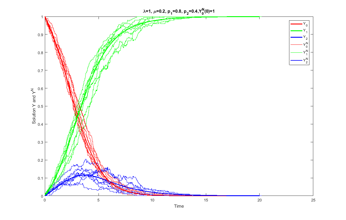
Typical sample paths of $Y^{N}$ are illustrated in Figure 1: When $N=200$ , $K=2$ , $\lambda=1$ , $\mu=0.2$ , $p_{1}=0.8$ , and $p_{2}=0.4$ , each of the component in $Y^{N}$ goes to their corresponding equilibrium states exponentially fast. In particular, these typical sample paths have two slightly different behaviors stages: At the first stage, $Y^{N}_{1}(t)$ and $Y^{N}_{2}(t)$ both increase up to the point where $Y^{N}_{1}(t)+Y^{N}_{2}(t)\approx 1$ – noting that $Y^{N}_{2}(t)$ grows much slower than $Y^{N}_{1}(t)$ . At the second stage, until entering their equilibrium states, $Y^{N}_{1}(t)$ is increasing and $Y^{N}_{2}(t)$ is decreasing. More importantly, $Y_{0}^{N},Y_{1}^{N},$ and $Y_{2}^{N}$ track their corresponding deterministic and smooth trajectories.

For fixed $K$ , $\lambda$ , and $p_{1}$ , $\lambda\left(\frac{\mu}{K}+(1-\mu)\right)p_{1}$ is decreasing in $\mu\in(0,1]$ . As a result of this, $R$ is also decreasing in $\mu$ . On the other hand, Theorem 3.1 presents a lower bound on the success probability, i.e., $\mathbb{P}\left\{E^{N}\right\}$ , which is increasing in $\mu$ . It is unclear whether there is indeed a fundamental trade-off between the success probability $\mathbb{P}\left\{E^{N}\right\}$ and the convergence rate $R$ or this is just an artifact of our analysis. As can be seen later, $\bar{t}_{c}$ is introduced for a technical reason.

Proof Sketch of Theorem 3.4.

We first show that for sufficiently large $N$ , the scaled Markov chains $\left(Y^{N}(t),t\in{\mathbb{R}}_{+}\right)$ (defined in (11)) can be approximated by the unique solution of an ODEs system. Define $F:\Delta^{K}\to{\mathbb{R}}^{K+1}$ as:

\displaystyle F(x)\triangleq\sum_{\ell\in{\mathbb{R}}^{K+1}}\ell\cdot f(x,\ell),~~\text{where }f\left(x,\ell\right)\triangleq\begin{cases}\lambda x_{0}\left(\frac{\mu}{K}+(1-\mu)x_{k}\right)p_{k},~~\text{if}~\ell=e^{k},~\forall~k\not=0;\\ \lambda x_{k^{\prime}}x_{k}p_{k},~~\text{if}~\ell=e^{k}-e^{k^{\prime}}\text{for}~k^{\prime}\not=k,k^{\prime}\not=0;\\ 0,~~~\text{otherwise}.\end{cases}

(12)

Intuitively, $f(x,\ell)$ is the rate to move in direction $\ell$ from the current scaled state $x\in\Delta^{K}$ , and function $F$ is the average movements of the scaled process $\left(Y^{N}(t),t\in{\mathbb{R}}_{+}\right)$ .

Lemma 3.5.

For a given $T$ , as the group size $N$ increases, the sequence of scaled random processes $\left(\frac{1}{N}X^{N}(t):t\in{\mathbb{R}}_{+}\right)$ converge, in probability, to a deterministic trajectory $Y(t)$ such that

\displaystyle\frac{\partial}{\partial t}Y(t)

\displaystyle=F\left(Y(t)\right),~~~t\in[0,T]

(13)

with initial condition $Y(0)=\left[1,0,\cdots,0\right]\in\Delta^{K}.$ In particular,

\displaystyle\mathbb{P}\left\{\sup_{0\leq t\leq T}\left\|{Y^{N}(t)-Y(t)}\right\|_{2}\geq~\epsilon^{\prime}\right\}\leq 2\left(K+1\right)\exp\left\{-N\cdot C(\epsilon^{\prime})\right\},

where $C(\epsilon^{\prime})=\frac{3-e}{9T\lambda}\frac{\left(\epsilon^{\prime}\right)^{2}}{(K+1)\exp\left(2\lambda\left(5+\sqrt{K}\right)T\right)}.$

Lemma 3.5 says that the scaled process $Y^{N}(t)$ , with high probability, closely tracks a deterministic and smooth trajectory. This coincides with simulation in Figure 1. The approximation in Lemma 3.5 is desired because the analysis of an ODEs system is relatively easier than that of the original stochastic system. Indeed, in a great variety of fields, such as biology, epidemic theory, physics, and chemistry [11], differential equations are used directly to model the macroscopic level system dynamics that are arguably caused by the microscopic level individuals interactions in the system.

For any $t\in[0,T]$ , the ODEs system $\frac{\partial}{\partial t}Y(t)=F\left(Y(t)\right)$ in (13) can be written out as:

	$\displaystyle\dot{Y_{0}}(t)$	$\displaystyle=-Y_{0}(t)\lambda\frac{\mu}{K}\sum_{k=1}^{k}p_{k}-Y_{0}(t)\lambda\sum_{k=1}^{K}(1-\mu)p_{k}Y_{k}(t),$		(14)
	$\displaystyle\dot{Y_{k}}(t)$	$\displaystyle=Y_{0}(t)\lambda\frac{\mu}{K}p_{k}+Y_{k}(t)\lambda\left((1-\mu)p_{k}Y_{0}(t)+\sum_{k^{\prime}=1}^{K}(p_{k}-p_{k^{\prime}})Y_{k^{\prime}}(t)\right),~~\forall k=1,\cdots,K.$		(15)

Note that our ODE system is quite different from the antisymmetric Lotka-Volterra equation [10]. The Lotka-Volterra equation is a typical replicator dynamics, where if $Y_{k}(0)=0$ for some $k$ , it remains to be zero throughout the entire process. In contrast, in our system, the desired ${\bf Y}^{*}=\left[Y_{0}^{*},Y_{1}^{*},\cdots,Y_{K}^{*}\right]=\left[0,1,0,\cdots,0\right]$ is achievable with $Y(0)=\left[1,0,\cdots,0\right]$ , and can be achieved exponentially fast.

Lemma 3.6.

With initial state $Y(0)=\left[1,0,\cdots,0\right]$ , the state ${\bf Y}^{*}=\left[0,1,0,\cdots,0\right]$ is achievable.

Lemma 3.7.

For any constant $c\in(0,1)$ , let $\bar{t}_{c}~\triangleq~\frac{\log\frac{1}{c}}{\lambda\frac{\mu}{K}\sum_{k^{\prime}=1}^{K}p_{k^{\prime}}}$ . When $t\geq\bar{t}_{c}$ , $Y(t)$ converges to ${\bf Y}^{*}=\left[0,1,0,\cdots,0\right]$ exponentially fast, with rate $\min\left\{\lambda\left(p_{1}-p_{2}\right),~\lambda\left(\frac{\mu}{K}+(1-\mu)\right)p_{1}\right\}$ .

By triangle inequality,

\displaystyle 1-Y_{1}^{N}(t)\leq\left\|{Y^{N}(t)-Y(t)}\right\|_{2}+\left|1-Y_{1}(t)\right|,~\text{and}~Y_{k}^{N}(t)\leq\left\|{Y^{N}(t)-Y(t)}\right\|_{2}+\left|Y_{k}(t)\right|,~~~\forall k\not=1.

Thus, Theorem 3.4 follows immediately from Lemmas 3.5, 3.6,and 3.7. ∎

4 Concluding Remarks

We studied the collaborative multi-armed bandit problems in social groups wherein each individual suffers finite memory constraint [6]. We rigorously investigated the power of persuasion, i.e., communication, in improving an individual’s learning capability. Similar learning dynamics are considered in [5] with the following fundamental differences.

•

We relax their synchronization assumption. It is assumed in [5] that time is slotted, and all individuals attempt to make one-step update simultaneously, where the updates are based on the system’s state at the end of previous round. This synchronization assumption imposed additional implementation challenges: Synchronization does not come for free. Typically the cost of synchronization depends deterministically on the slowest individual in the system.

In contrast, our work relaxes this synchronization assumption and considers the less restrictive asynchronous setting where each individual has an independent Poisson clock, and attempts to perform a one-step update immediately when its local clock ticks. The Poisson clock model is very natural: The real world is an asynchronous one and there are physical reasons to use a modeling approach based on Poisson clocks [21]. This model avoids the implementation challenges in [5], nevertheless, it causes non-trivial analysis challenge – we have to deal with the stochastic dependency among any updates. In contrast, with synchronization, the individuals’ updates of the same round in [5] are conditionally independent.
•

We relax the requirement of performing uniform sampling by all individuals, and we are able to show learnability of every individual. It is assumed in [5] that, in each round, every individual, regardless of its preference states, performs uniform sampling with probability $\mu$ . This assumption is imposed for a technical reason: They wanted to “ensure that the population does not get stuck in a bad option”. However, as a result of their assumption, as $t\to\infty$ , there is a constant fraction $\mu\in(0,1]$ of individuals that cannot learn the best option. In contrast, in our learning dynamics, we require only that the individuals without any preference do uniform sampling. We overcome their concerns of “get stuck in a bad option” by showing that such events occur with probability diminishing to $0$ as the social group size $N\to\infty$ .
•

We use the mean-field approximation method to provide a provable connection between the finite and the infinite population dynamics. In [5], the authors first define an “infinite population” version of their dynamics and then translate its convergence properties to the finite population stochastic dynamics. Unfortunately, the connection between their infinite and the finite population dynamics is only established through the “non-rigorous thought process” – as the authors themselves commented [5]. Similar heuristic arguments were also made in the evolutionary biology literature [9]. In contrast, we use the mean-field approximation method to provide a provable connection between these two dynamics.

Acknowledgements

We would like to thank John N. Tsitsiklis for valuable discussions and comments.

References

[1] Auer, P., Cesa-Bianchi, N., and Fischer, P. Finite-time analysis of the multiarmed bandit problem. Machine learning 47, 2-3 (2002), 235–256.
[2] Bandura, A. Social-learning theory of identificatory processes. Handbook of socialization theory and research 213 (1969), 262.
[3] Bergemann, D., and V�lim�ki, J. Learning and strategic pricing. Econometrica 64, 5 (1996), 1125–1149.
[4] Bubeck, S., Cesa-Bianchi, N., et al. Regret analysis of stochastic and nonstochastic multi-armed bandit problems. Foundations and Trends® in Machine Learning 5, 1 (2012), 1–122.
[5] Celis, L. E., Krafft, P. M., and Vishnoi, N. K. A distributed learning dynamics in social groups. In Proceedings of the ACM Symposium on Principles of Distributed Computing (New York, NY, USA, 2017), PODC ’17, ACM, pp. 441–450.
[6] Cover, T., and Hellman, M. The two-armed-bandit problem with time-invariant finite memory. IEEE Transactions on Information Theory 16, 2 (March 1970), 185–195.
[7] Cover, T. M. A note on the two-armed bandit problem with finite memory. Information and Control 12, 5 (1968), 371–377.
[8] Hajek, B. Random processes for engineers. Cambridge University Press, 2015.
[9] Kang, Y., and Theraulaz, G. Dynamical models of task organization in social insect colonies. Bulletin of mathematical biology 78, 5 (2016), 879–915.
[10] Knebel, J., Weber, M. F., Krüger, T., and Frey, E. Evolutionary games of condensates in coupled birth–death processes. Nature communications 6 (2015).
[11] Kurtz, T. G. Solutions of ordinary differential equations as limits of pure jump markov processes. Journal of applied Probability 7, 1 (1970), 49–58.
[12] Kurtz, T. G. Approximation of population processes. SIAM, 1981.
[13] Lai, T. L., and Robbins, H. Asymptotically efficient adaptive allocation rules. Advances in applied mathematics 6, 1 (1985), 4–22.
[14] Mannor, S., and Tsitsiklis, J. N. The sample complexity of exploration in the multi-armed bandit problem. Journal of Machine Learning Research 5, Jun (2004), 623–648.
[15] Mitzenmacher, M. D. The Power of Two Choices in Randomized Load Balancing. PhD thesis, UNIVERSITY of CALIFORNIA at BERKELEY, 1996.
[16] Musco, C., Su, H.-H., and Lynch, N. A. Ant-inspired density estimation via random walks. Proceedings of the National Academy of Sciences 114, 40 (2017), 10534–10541.
[17] Nakayama, K., Hisakado, M., and Mori, S. Nash equilibrium of social-learning agents in a restless multiarmed bandit game. Scientific Reports 7 (2017).
[18] Pini, G., Brutschy, A., Francesca, G., Dorigo, M., and Birattari, M. Multi-armed bandit formulation of the task partitioning problem in swarm robotics. In ANTS (2012), Springer, pp. 109–120.
[19] Rendell, L., Boyd, R., Cownden, D., Enquist, M., Eriksson, K., Feldman, M. W., Fogarty, L., Ghirlanda, S., Lillicrap, T., and Laland, K. N. Why copy others? insights from the social learning strategies tournament. Science 328, 5975 (2010), 208–213.
[20] Robbins, H. A sequential decision problem with a finite memory. Proceedings of the National Academy of Sciences 42, 12 (1956), 920–923.
[21] Ross, S. M. Introduction to probability models. Academic press, 2014.
[22] Shen, W., Wang, J., Jiang, Y.-G., and Zha, H. Portfolio choices with orthogonal bandit learning. In IJCAI (2015), p. 974.
[23] Shwartz, A., and Weiss, A. Large deviations for performance analysis: queues, communication and computing, vol. 5. CRC Press, 1995.
[24] Smith, C. V., and Pyke, R. The robbins-isbell two-armed-bandit problem with finite memory. The Annals of Mathematical Statistics (1965), 1375–1386.
[25] Stanley, H. E. Phase transitions and critical phenomena. Clarendon, Oxford 9 (1971).
[26] Su, H.-H., Su, L., Dornhaus, A., and Lynch, N. Ant-inspired dynamic task allocation via gossiping.
[27] Xu, K., and Yun, S.-Y. Reinforcement with fading memories. In Sigmetrics (2018).

Appendix A Space-Time Structure

Recall that a time-homogeneous, discrete-state Markov chain (can possibly be continuous-time or discrete-time) can be described alternatively by specifying its space-time structure [8], which is simply the sequence of states visited (jump process) and how long each state is stayed at per visit (holding times).

Let $H_{l}$ be the time that elapses between the $l^{th}$ and the ${l+1}^{th}$ jumps of $\left(X^{N}(t):t\in{\mathbb{R}}_{+}\right)$ . Intuitively, $H_{l}$ is the amount of time that the process is “held” by the $l^{th}$ jump. More formally,

	$\displaystyle H_{0}$	$\displaystyle=\min_{t}\left\{t\geq 0:~X^{N}(t)\not=X^{N}(0)\right\}$		(16)
	$\displaystyle H_{l}$	$\displaystyle=\min_{t}\left\{t\geq 0:~X^{N}(H_{0}+\cdots+H_{l-1}+t)\not=X^{N}(H_{0}+\cdots+H_{l-1})\right\},$		(17)

as the $l^{th}$ jump occurs at time $H_{0}+\cdots+H_{l-1}$ and the ${l+1}^{th}$ jump occurs at time $H_{0}+\cdots+H_{l}$ . Correspondingly, the jump process embedded in the continuous-time Markov chain $X^{N}(t)$ is defined by

\displaystyle X^{J,N}(0)=X^{N}(0)~~~~\text{and}~~~~X^{J,N}(l)=X^{N}(H_{0}+\cdots+H_{l-1}),

(18)

with

\displaystyle X^{J,N}(l)

\displaystyle=\left[X^{J,N}_{0}(l),X^{J,N}_{1}(l),\cdots,X^{J,N}_{K}(l)\right],

(19)

where $X^{J,N}_{k}(l),$ is the number of individuals that prefer arm $a_{k}$ at the $l^{th}$ jump. The holding times $\{H_{l}\}_{l=0}^{\infty}$ and the jump process $\left(X^{J,N}(l):l\in{\mathbb{Z}}_{+}\right)$ contain all the information needed to reconstruct the original Markov chain $X^{N}(t)$ , and vice versa [8].

Proposition 2.

[8] Let $\left(X(t):t\in{\mathbb{R}}_{+}\right)$ be a time-homogeneous, pure-jump Markov process with generator matrix $Q$ . Then the jump process $X^{J}$ is a discrete-time, time-homogeneous Markov process, and its one-step transition probabilities are given by

\displaystyle p_{ss^{\prime}}^{J}=\begin{cases}-\frac{q_{ss^{\prime}}}{q_{ss}},&\mbox{for }s\not=s^{\prime};\\ 0,&\mbox{for }s=s^{\prime},\end{cases}

(20)

with the convention that $\frac{0}{0}\triangleq 0$ .

Our analysis will also use the space-time structure of the discrete-time Markov chain, as we will use such structure of the above derived jump process $X^{J}$ .

Proposition 3.

[8] Let $\left(X(k):k\in{\mathbb{Z}}_{+}\right)$ be a time-homogeneous Markov process with one-step transition probability matrix $P$ . Then the jump process $\left(X^{J}(l):l\in{\mathbb{Z}}_{+}\right)$ is itself a time-homogeneous Markov process, and its one-step transition probabilities are given by

\displaystyle p_{ss^{\prime}}^{J}=\begin{cases}\frac{p_{ss^{\prime}}}{1-p_{ss}},&\mbox{for }s\not=s^{\prime};\\ 0,&\mbox{for }s=s^{\prime},\end{cases}

(21)

with the convention that $\frac{0}{0}\triangleq 0$ .

Appendix B Learnability

B.1 Proof of Lemma 3.2

The proof of Lemma 3.2 uses the following claim.

Claim 1.

For any $c\geq 0$ , $y>0$ , $x+y>0$ and $x+y+c>0$ , it holds that

\displaystyle\frac{x}{x+y}

\displaystyle<\frac{x+c}{x+c+y}.

Proof.

The proof of this claim is elementary, and is presented for completeness.

\displaystyle\frac{x+c}{x+c+y}-\frac{x}{x+y}

\displaystyle=1-\frac{y}{x+c+y}-1+\frac{y}{x+y}=y\left(\frac{1}{x+y}-\frac{1}{x+c+y}\right)\geq 0.

∎

Now we are ready to prove Lemma 3.2.

Proof of Lemma 3.2.

For ease of exposition, for a fixed $k\in{\mathbb{Z}}_{+}$ , define

\displaystyle A^{k}\triangleq\left\{\omega:W(k+1)=W(k)+1~\text{given }~W(k)\notin\{0,N\}\right\}.

(22)

To show Lemma 3.2, it is enough to show $\mathbb{P}\left\{A^{k}\right\}\geq\frac{p_{1}}{p_{1}+p_{2}}$ .

We first link the random walk back to the first order space-time structure of the original continuous-time Markov chain as follows:

	$\displaystyle A^{k}$	$\displaystyle=\left\{\omega:W(k+1)=W(k)+1~\text{given }W(k)\notin\{0,N\}\right\}$
		$\displaystyle=\cup_{l=1}^{\infty}\Big\{\omega:\text{the $k+1^{th}$ move of $W$ occurs at the ${l+1}^{th}$ jump of $X^{J,N}$ }$
		$\displaystyle~~~~~~~~~~~~~~~\&~X^{J,N}_{1}(l+1)=X^{J,N}_{1}(l)+1~\text{given }W(k)\notin\{0,N\}~~~~~~~~\Big\}.$

For ease of exposition, define $B^{k}_{l}$ as

$\displaystyle B^{k}_{l}$	$\displaystyle\triangleq\Big\{\omega:\text{the $k+1^{th}$ move of $W$ occurs at the ${l+1}^{th}$ jump of $X^{J,N}$ }$
	$\displaystyle~~~~~~~~~\&~X^{J,N}_{1}(l+1)=X^{J,N}_{1}(l)+1~\text{given }W(k)\notin\{0,N\}~~~~~~~~\Big\}$
	$\displaystyle=\Big\{\omega:\text{the $k+1^{th}$ move of $W$ occurs at the ${l+1}^{th}$ jump of $X^{J,N}$ }$
	$\displaystyle~~~~~~~~~\&~X^{J,N}_{1}(l+1)=X^{J,N}_{1}(l)+1~\text{given }X^{J,N}_{1}(l)\notin\{0,N\}~~~~~~~~\Big\}.$	(23)

It is easy to see that $B^{k}_{l}=\O~\text{for }l<k$ . So we get $A^{k}=\cup_{l\geq k}~B^{k}_{l}.$ In addition, by definition, $B^{k}_{l}\cap B^{k}_{l^{\prime}}=\O,\forall~l\not=l^{\prime}$ . Thus,

\displaystyle\mathbb{P}\left\{A^{k}\right\}=\mathbb{P}\left\{\cup_{l\geq k}B_{l}^{k}\right\}=\sum_{l\geq k}\mathbb{P}\left\{B_{l}^{k}\right\}.

(24)

Now we focus on $\mathbb{P}\left\{B_{l}^{k}\right\}$ . Let ${\mathcal{S}}^{N}$ be the collection of valid states such that for every $s\in{\mathcal{S}}^{N}$ , $s_{1}\notin\{0,N\}$ – recalling that a valid state is a partition of integer $N$ . By total probability argument, we have

\displaystyle\mathbb{P}\left\{B_{l}^{k}\right\}

\displaystyle=\sum_{s\in{\mathcal{S}}^{N}}\mathbb{P}\left\{X^{J,N}(l)=s\mid X^{J,N}_{1}(l)\notin\{0,N\}\right\}\mathbb{P}\left\{B_{l}^{k}\mid X^{J,N}(l)=s\right\},

(25)

where

\displaystyle\sum_{s\in{\mathcal{S}}^{N}}\mathbb{P}\left\{X^{J,N}(l)=s\mid X^{J,N}_{1}(l)\notin\{0,N\}\right\}=1.

(26)

Define event $C_{l}^{k}$ as follow:

\displaystyle C^{k}_{l}\triangleq\left\{\omega:\text{the $k+1^{th}$ move of $W$ occurs at the ${l+1}^{th}$ jump of $X^{J,N}$ given $X^{J,N}_{1}(l)\notin\{0,N\}$}\right\}.

(27)

It is easy to see that for a fixed $k$ ,

\displaystyle\sum_{l\geq k}\mathbb{P}\left\{C^{k}_{l}\right\}=1.

(28)

For $l\geq k$ , we have

\displaystyle\mathbb{P}\left\{B_{l}^{k}\mid X^{J,N}(l)=s\right\}=\mathbb{P}\left\{C_{l}^{k}\mid X^{J,N}(l)=s\right\}\mathbb{P}\left\{X^{J,N}_{1}(l+1)=X^{J,N}_{1}(l)+1\mid C_{l}^{k},X^{J,N}(l)=s\right\}.

(29)

We claim that

\displaystyle\mathbb{P}\left\{X^{J,N}_{1}(l+1)=X^{J,N}_{1}(l)+1\mid C_{l}^{k},X^{J,N}(l)=s\right\}\geq\frac{p_{1}}{p_{1}+p_{2}}.

(30)

We postpone the proof of (30) to the end of the proof of Lemma 3.2. With (30), we are able to conclude that $\mathbb{P}\left\{A^{k}\right\}\geq\frac{p_{1}}{p_{1}+p_{2}}$ . In particular, equation (29) becomes

\displaystyle\mathbb{P}\left\{B_{l}^{k}\mid X^{J,N}(l)=s\right\}

\displaystyle\geq\mathbb{P}\left\{C_{l}^{k}\mid X^{J,N}(l)=s\right\}\frac{p_{1}}{p_{1}+p_{2}}.

(31)

By (24), (25) and (31), we have

	$\displaystyle\mathbb{P}\left\{A^{k}\right\}$	$\displaystyle=\sum_{l\geq k}\sum_{s\in{\mathcal{S}}^{N}}\mathbb{P}\left\{X^{J,N}(l)=s\mid X^{J,N}_{1}(l)\notin\{0,N\}\right\}\mathbb{P}\left\{B_{l}^{k}\mid X^{J,N}(l)=s\right\}$
		$\displaystyle\geq\sum_{l\geq k}\sum_{s\in{\mathcal{S}}^{N}}\mathbb{P}\left\{X^{J,N}(l)=s\mid X^{J,N}_{1}(l)\notin\{0,N\}\right\}\mathbb{P}\left\{C_{l}^{k}\mid X^{J,N}(l)=s\right\}\frac{p_{1}}{p_{1}+p_{2}}$
		$\displaystyle=\frac{p_{1}}{p_{1}+p_{2}}\sum_{l\geq k}\sum_{s\in{\mathcal{S}}^{N}}\mathbb{P}\left\{X^{J,N}(l)=s,C_{l}^{k}\right\}$
		$\displaystyle=\frac{p_{1}}{p_{1}+p_{2}}\sum_{l\geq k}\sum_{s\in{\mathcal{S}}^{N}}\mathbb{P}\left\{C_{l}^{k}\right\}\mathbb{P}\left\{X^{J,N}(l)=s\mid C_{l}^{k}\right\}$
		$\displaystyle=\frac{p_{1}}{p_{1}+p_{2}},$

where the last equality follows from (26) and (28).

Next we prove (30). We have

		$\displaystyle\mathbb{P}\left\{X^{J,N}_{1}(l+1)=X^{J,N}_{1}(l)+1\mid C_{l}^{k},X^{J,N}(l)=s\right\}$
		$\displaystyle=\mathbb{P}\big\{X^{J,N}_{1}(l+1)=X^{J,N}_{1}(l)+1\mid X^{J,N}(l)=s,s_{1}\notin\{0,N\},\text{the $k+1^{th}$ move of $W$}$
		$\displaystyle~~~~~~~~~~~~~~~~~~~~~~~~~~~~~~~~~~~~~~~~~~~~\text{occurs at the $l+1^{th}$ jump of $X^{J,N}$ given $W(k)\notin\{0,N\}$}\big\}$
		$\displaystyle=\mathbb{P}\big\{X^{J,N}_{1}(l+1)=X^{J,N}_{1}(l)+1\mid X^{J,N}(l)=s,s_{1}\notin\{0,N\}$
		$\displaystyle~~~~~~~~~~~~~~~~~~~~~~~~~~~~~~~~~~~~~~~~~~~~\text{one move of $W$ occurs at the $l+1^{th}$ jump of $X^{J,N}$},$
		$\displaystyle~~~~~~~~~~~~~~~~~~~~~~~~~~~~~~~~~~~~~~~~~~~~\text{and there are $k$ moves of $W$ occur among the first $l$ jumps of $X^{J,N}$}\big\}$
		$\displaystyle\overset{(a)}{=}\mathbb{P}\big\{X^{J,N}_{1}(l+1)=X^{J,N}_{1}(l)+1\mid X^{J,N}(l)=s,s_{1}\notin\{0,N\}$
		$\displaystyle~~~~~~~~~~~~~~~~~~~~~~~~~~~~~~~~~~~~~~~~~~~~\text{one move of $W$ occurs at the $l+1^{th}$ jump of $X^{J,N}$}\big\}$
		$\displaystyle=\frac{\mathbb{P}\left\{X^{J,N}_{1}(l+1)=X^{J,N}_{1}(l)+1\mid X^{J,N}(l)=s,s\in{\mathcal{S}}^{N}\right\}}{\mathbb{P}\left\{\text{one move of $W$ occurs at the $l+1^{th}$ jump of $X^{J,N}$}\mid X^{J,N}(l)=s,s\in{\mathcal{S}}^{N}\right\}},$		(32)

where equality (a) follows from the Markov property of $X^{J,N}$ . By Proposition 2, we know

\displaystyle\mathbb{P}\left\{X^{J,N}_{1}(l+1)=X^{J,N}_{1}(l)+1\mid X^{J,N}(l)=s,s\in{\mathcal{S}}^{N}\right\}=-\sum_{s^{\prime}:s_{1}^{\prime}=s_{1}+1}\frac{q_{s,s^{\prime}}}{q_{s,s}}.

(33)

Note that $\sum_{s^{\prime}:s_{1}^{\prime}=s_{1}+1}q_{s,s^{\prime}}$ is exactly the birth rate of the best arm, i.e., arm $a_{1}$ . That is,

\displaystyle\sum_{s^{\prime}:s_{1}^{\prime}=s_{1}+1}q_{s,s^{\prime}}=s_{0}\lambda\left(\frac{\mu}{K}+\left(1-\mu\right)\frac{s_{1}}{N}\right)p_{1}+\sum_{j\geq 2}s_{j}\lambda\frac{s_{1}}{N}p_{1}.

(34)

Similarly,

\displaystyle\mathbb{P}\left\{\text{one move of $W$ occurs at the $l+1^{th}$ jump of $X^{J,N}$}\mid X^{J,N}(l)=s,s\in{\mathcal{S}}^{N}\right\}

\displaystyle=-\sum_{s^{\prime}:s_{1}^{\prime}=s_{1}\pm 1}\frac{q_{s,s^{\prime}}}{q_{s,s}},

(35)

and $\sum_{s^{\prime}:s_{1}^{\prime}=s_{1}\pm 1}q_{s,s^{\prime}}$ is the summation of birth rate and death rate of the best arm. Specifically,

\displaystyle\sum_{s^{\prime}:s_{1}^{\prime}=s_{1}\pm 1}q_{s,s^{\prime}}=s_{0}\lambda\left(\frac{\mu}{K}+\left(1-\mu\right)\frac{s_{1}}{N}\right)p_{1}+\sum_{j\geq 2}s_{j}\lambda\frac{s_{1}}{N}p_{1}+s_{1}\lambda\sum_{j\geq 2}\frac{s_{j}}{N}p_{j}.

(36)

Thus, by (32), (33) and (35), we have

\displaystyle\mathbb{P}\left\{X^{J,N}_{1}(l+1)=X^{J,N}_{1}(l)+1\mid C_{l}^{k},X^{J,N}(l)=s\right\}

\displaystyle=\frac{-\sum_{s^{\prime}:s_{1}^{\prime}=s_{1}+1}\frac{q_{s,s^{\prime}}}{q_{s,s}}}{-\sum_{s^{\prime}:s_{1}^{\prime}=s_{1}\pm 1}\frac{q_{s,s^{\prime}}}{q_{s,s}}}=\frac{\sum_{s^{\prime}:s_{1}^{\prime}=s_{1}+1}q_{s,s^{\prime}}}{\sum_{s^{\prime}:s_{1}^{\prime}=s_{1}\pm 1}q_{s,s^{\prime}}},

and by (34) and (36), we have

		$\displaystyle\mathbb{P}\left\{X^{J,N}_{1}(l+1)=X^{J,N}_{1}(l)+1\mid C_{l}^{k},X^{J,N}(l)=s\right\}$
		$\displaystyle=\frac{s_{0}\lambda\left(\frac{\mu}{K}+\left(1-\mu\right)\frac{s_{1}}{N}\right)p_{1}+\sum_{j\geq 2}s_{j}\lambda\frac{s_{1}}{N}p_{1}}{s_{0}\lambda\left(\frac{\mu}{K}+\left(1-\mu\right)\frac{s_{1}}{N}\right)p_{1}+\sum_{j\geq 2}s_{j}\lambda\frac{s_{1}}{N}p_{1}+s_{1}\lambda\sum_{j\geq 2}\frac{s_{j}}{N}p_{j}}$
		$\displaystyle=\frac{s_{0}\left(\frac{\mu}{K}+(1-\mu)\frac{s_{1}}{N}\right)p_{1}+(N-s_{1}-s_{0})\frac{s_{1}}{N}p_{1}}{s_{0}\left(\frac{\mu}{K}+(1-\mu)\frac{s_{1}}{N}\right)p_{1}+(N-s_{1}-s_{0})\frac{s_{1}}{N}p_{1}+s_{1}\sum_{j\geq 2}\frac{s_{j}}{N}p_{j}}$
		$\displaystyle\overset{(a)}{\geq}\frac{s_{0}(1-\mu)\frac{s_{1}}{N}p_{1}+(N-s_{1}-s_{0})\frac{s_{1}}{N}p_{1}}{s_{0}(1-\mu)\frac{s_{1}}{N}p_{1}+(N-s_{1}-s_{0})\frac{s_{1}}{N}p_{1}+s_{1}\sum_{j\geq 2}\frac{s_{j}}{N}p_{j}}$
		$\displaystyle=\frac{(N-s_{1}-\mu s_{0})p_{1}}{(N-s_{1}-\mu s_{0})p_{1}+\sum_{j\geq 2}s_{j}p_{j}},$		(37)

where inequality (a) follows from Claim 1. In addition, we have

\displaystyle\sum_{j\geq 2}s_{j}p_{j}

\displaystyle\leq\sum_{j\geq 2}s_{j}p_{2}=(N-s_{0}-s_{1})p_{2}\leq(N-\mu s_{0}-s_{1})p_{2}.

So (37) becomes

	$\displaystyle\mathbb{P}\left\{X^{J,N}_{1}(l+1)=X^{J,N}_{1}(l)+1\mid C_{l}^{k},X^{J,N}(l)=s\right\}$	$\displaystyle>\frac{(N-s_{1}-\mu s_{0})p_{1}}{(N-s_{1}-\mu s_{0})p_{1}+(N-\mu s_{0}-s_{1})p_{2}}$
		$\displaystyle=\frac{p_{1}}{p_{1}+p_{2}},$

proving (30).

Therefore, the proof of Lemma 3.2 is complete.

∎

B.2 Coupling

Recall that random walk $\left(\widehat{W}(k):\,k\in{\mathbb{Z}}_{+}\right)$ defined in (10): If $\widehat{W}(k)=0$ or $\widehat{W}(k)=N$ , then $\widehat{W}(k+1)=\widehat{W}(k)$ ; Otherwise,

\displaystyle\widehat{W}(k+1)=\begin{cases}\widehat{W}(k)+1~&\text{with probability }\frac{p_{1}}{p_{1}+p_{2}};\\ \widehat{W}(k)-1~&\text{with probability }\frac{p_{2}}{p_{1}+p_{2}}.\end{cases}

Intuitively, the embedded random walk has a higher tendency to move one step up (if possible) than that of the standard random walk (10). Thus, starting at the same position, the embedded random walk should have a higher chance to be absorbed at position $N$ . Formal coupling argument is given below.

From Propositions 2 and 3, we know that the transition probability of the embedded random walk $\left(W(k):\,k\in{\mathbb{Z}}_{+}\right)$ is determined by the entire state (which is random) of the original continuous-time Markov chain $\left(X^{N}(t):\,t\in{\mathbb{R}}_{+}\right)$ right proceeding the $k^{th}$ move of $\left(W(k):\,k\in{\mathbb{Z}}_{+}\right)$ .

Let $x^{N}(\cdot)=\left[x_{0}^{N}(\cdot),x_{1}^{N}(\cdot),\cdots,x_{K}^{N}(\cdot)\right]$ be an arbitrary sample path of $\left(X^{N}(t):\,t\in{\mathbb{R}}_{+}\right)$ such that only one jump occurs at a time and no jumps occur at time $t_{c}=\frac{1}{\lambda}$ . Note that $x^{N}(\cdot)$ is a vector-valued function defined over ${\mathbb{R}}_{+}$ . Clearly, with probability one, a sample path of $\left(X^{N}(t):\,t\in{\mathbb{R}}_{+}\right)$ satisfies these conditions. We focus on the coordinate process $x_{1}^{N}(\cdot)$ – the evolution of the number of individuals that prefer the best option. Given $x_{1}^{N}(\cdot)$ , the sample path of the embedded random walk $\left(\widehat{W}(k):\,k\in{\mathbb{Z}}_{+}\right)$ , denoted by $w(k),\forall k\in{\mathbb{Z}}_{+}$ , is also determined. Note that $w(\cdot)$ is defined over ${\mathbb{Z}}_{+}$ .

Let $\tau_{j}$ for $j=1,2,\cdots$ be the $j^{th}$ jump time during $(t_{c},\infty)$ , where $t_{c}=\frac{1}{\lambda}$ . The time $t_{c}$ is referred as coupling starting time. For ease of notation, let

\displaystyle\lim_{h\downarrow 0}x^{N}(\tau_{j}-h)~\triangleq~\widetilde{x}(\tau_{j})=\left[\widetilde{x}^{N}_{0}(\tau_{j}),\widetilde{x}^{N}_{1}(\tau_{j}),\cdots,x^{N}_{K}(\tau_{j})\right].

(38)

We couple $\left(W(k):\,k\in{\mathbb{Z}}_{+}\right)$ and $\left(\widehat{W}(k):\,k\in{\mathbb{Z}}_{+}\right)$ as follows: Let

\displaystyle\widehat{w}(0)=x_{1}^{N}(t_{c}).

(39)

•

If the embedded random walk $\left(W(k):\,k\in{\mathbb{Z}}_{+}\right)$ moves one position down in the sample path $x^{N}(t)$ , then we move the standard random walk $\left(\widehat{W}:\,k\in{\mathbb{Z}}_{+}\right)$ one position down if possible. (If the standard random walk is at zero already, it stays at zero.)

•

If the embedded random walk $\left(W(k):\,k\in{\mathbb{Z}}_{+}\right)$ moves one position up in the sample path $x^{N}(t)$ , then we move the standard random walk $\left(\widehat{W}(k):\,k\in{\mathbb{Z}}_{+}\right)$ one position up. Then we flip a biased coin whose probability of showing head is a function of the state of $\widetilde{x}^{N}(\tau_{j})$ . If “HEAD”, the standard random walk stays at where it is, otherwise (“TAIL”), the standard random walk moves two positions down. In particular,

\displaystyle\begin{cases}\text{HEAD},&\text{with probability }\frac{p_{1}}{(p_{1}+p_{2})\eta(\tau_{j})};\\ \text{TAIL},&\text{with probability }1-\frac{p_{1}}{(p_{1}+p_{2})\eta(\tau_{j})},\end{cases}

where

\displaystyle\eta(\tau_{j})\triangleq\frac{\widetilde{x}_{0}^{N}(\tau_{j})\left(\frac{\mu}{K}+(1-\mu)\frac{\widetilde{x}_{1}^{N}(\tau_{j})}{N}\right)p_{1}+\sum_{k\geq 2}\widetilde{x}_{k}^{N}(\tau_{j})\frac{\widetilde{x}_{1}^{N}(\tau_{j})}{N}p_{1}}{\widetilde{x}_{0}^{N}(\tau_{j})\left(\frac{\mu}{K}+(1-\mu)\frac{\widetilde{x}_{1}^{N}(\tau_{j})}{N}\right)p_{1}+\sum_{k\geq 2}\widetilde{x}_{k}^{N}(\tau_{j})\frac{\widetilde{x}_{1}^{N}(\tau_{j})}{N}p_{1}+\widetilde{x}_{1}^{N}(\tau_{j})\sum_{k\geq 2}\frac{\widetilde{x}_{k}^{N}(\tau_{j})}{N}p_{k}}.

It is easy to see that the above construction is a valid coupling.

B.3 Proof of Lemma 3.3

We define a collection of $i.i.d.$ Bernoulli random variables and conclude the proof with applying Chernoff bound. For a given $t_{c}$ and for each $n=1,\cdots,N$ , let

\displaystyle Z_{n}(t_{c})=\bm{1}_{\left\{\text{individual $n$ wakes up only once during time $[0,t_{c}]$ and $M_{n}(t_{c})=1$}\right\}}.

(40)

Since an individual wakes up whenever its Poisson clock ticks and the Poisson clocks are independent among individuals, we know that $Z_{n}(t_{c}),\forall~n=1,\cdots,N$ are independent. In addition, by symmetry, $Z_{n}(t_{c}),\forall~n=1,\cdots,N$ are identically distributed. Recall that $X_{1}^{N}(t_{c})$ is the number of individuals whose memory states are $1$ at time $t_{c}$ , which includes the individuals that wake up multiple times. Thus, we have

\displaystyle X_{1}^{N}(t_{c})\geq\sum_{n=1}^{N}Z_{n}(t_{c}).

(41)

Next we bound $\mathbb{E}\left[Z_{n}(t_{c})\right]$ .

$\displaystyle\mathbb{E}\left[Z_{n}(t_{c})\right]$	$\displaystyle=\mathbb{P}\left\{\text{individual $n$ wakes up only once during time $[0,t_{c}]$ and $M_{n}(t_{c})=1$}\right\}$
	$\displaystyle=\mathbb{P}\left\{\text{individual $n$ wakes up only once during $[0,t_{c}]$}\right\}$
	$\displaystyle~~~\times\mathbb{P}\left\{\text{individual $n$ updates $M$ to 1 $\mid$ individual $n$ wakes up only once during $[0,t_{c}]$}\right\}$
	$\displaystyle\geq\frac{\left(t_{c}\lambda\right)^{1}\exp\{-t_{c}\lambda\}}{1}\times\frac{\mu}{K}p_{1}.$	(42)

When $t_{c}=\frac{1}{\lambda}$ , we have

\displaystyle\mathbb{E}\left[Z_{n}\left(\frac{1}{\lambda}\right)\right]\geq\frac{\mu p_{1}}{Ke}.

(43)

In fact that the lower bound in (42) is maximized by the choice of $t_{c}=\frac{1}{\lambda}$ . For any $0<\delta<1$ we have

	$\displaystyle\mathbb{P}\left\{\sum_{n=1}^{N}Z_{n}\left(\frac{1}{\lambda}\right)\geq(1-\delta)\frac{\mu p_{1}}{Ke}N\right\}$	$\displaystyle\geq\mathbb{P}\left\{\sum_{n=1}^{N}Z_{n}\left(\frac{1}{\lambda}\right)\geq(1-\delta)\mathbb{E}\left[Z_{n}\left(\frac{1}{\lambda}\right)\right]N\right\}$
		$\displaystyle=1-\mathbb{P}\left\{\sum_{n=1}^{N}Z_{n}\left(\frac{1}{\lambda}\right)<(1-\delta)\mathbb{E}\left[Z_{n}\left(\frac{1}{\lambda}\right)\right]N\right\}$
		$\displaystyle\overset{(a)}{\geq}1-e^{-\frac{\delta^{2}}{2}\mathbb{E}\left[Z_{n}\left(\frac{1}{\lambda}\right)\right]N}$
		$\displaystyle\geq 1-e^{-\frac{\mu p_{1}}{Ke}\frac{\delta^{2}}{2}N},$

where inequality (a) follows from Chernoff bound, and the last inequality follows from (43).

Therefore, for any $0<\delta<1$ we have

\displaystyle\mathbb{P}\left\{X_{1}^{N}\left(\frac{1}{\lambda}\right)\geq(1-\delta)\frac{\mu p_{1}}{Ke}N\right\}\geq 1-e^{-\frac{\mu p_{1}}{Ke}\frac{\delta^{2}}{2}N}.

B.4 Proof of Theorem 3.1

With Proposition 1 and Lemma 3.3, we are ready to show learnability under the learning dynamics in Algorithm 1. Recall from (8) that

\displaystyle E^{N}\triangleq\left\{\lim_{t\to\infty}X^{N}(t)=x^{*}\right\}=\left\{\lim_{l\to\infty}X_{1}^{J,N}(l)=N\right\}

\displaystyle\subseteq\left\{\text{every individual learns the best option}\right\}.

Proof.

With the choice of coupling starting time $t_{c}=\frac{1}{\lambda}$ , we have

		$\displaystyle\mathbb{P}\left\{\text{every individual learns the best option}\right\}\geq\mathbb{P}\left\{E^{N}\right\}=\mathbb{P}\left\{\lim_{t\to\infty}X^{N}(t)=x^{*}\right\}$
		$\displaystyle=\left\{\lim_{l\to\infty}X_{1}^{J,N}(l)=N\right\}$
		$\displaystyle\geq\mathbb{P}\left\{X^{N}_{1}\left(\frac{1}{\lambda}\right)\geq(1-\delta)\frac{\mu p_{1}}{Ke}N,~\&~\lim_{l\to\infty}X_{1}^{J,N}(l)=N\right\}$
		$\displaystyle=\mathbb{P}\left\{X^{N}_{1}\left(\frac{1}{\lambda}\right)\geq(1-\delta)\frac{\mu p_{1}}{Ke}N\right\}\mathbb{P}\left\{\lim_{l\to\infty}X_{1}^{J,N}(l)=N\mid X^{N}_{1}\left(\frac{1}{\lambda}\right)\geq(1-\delta)\frac{\mu p_{1}}{Ke}N\right\}$
		$\displaystyle\geq(1-e^{-\frac{\mu p_{1}}{Ke}\frac{\delta^{2}}{2}N})\mathbb{P}\left\{\lim_{l\to\infty}X_{1}^{J,N}(l)=N\mid X^{N}_{1}\left(\frac{1}{\lambda}\right)\geq(1-\delta)\frac{\mu p_{1}}{Ke}N\right\},$		(44)

where the last inequality follows from Lemma 3.3. In addition, we have

		$\displaystyle\left\{\lim_{k\to\infty}W(k)=N\text{ and }W(k)>0\text{ after time $\frac{1}{\lambda}$}\mid X^{N}\left(\frac{1}{\lambda}\right)\geq(1-\delta)\frac{\mu p_{1}}{Ke}N\right\}$
		$\displaystyle\subseteq\left\{\lim_{l\to\infty}X_{1}^{J,N}(l)=N\mid X^{N}_{1}\left(\frac{1}{\lambda}\right)\geq(1-\delta)\frac{\mu p_{1}}{Ke}N\right\}.$

By construction of our coupling, with the coupling starting time $t_{c}=\frac{1}{\lambda}$ , we have

		$\displaystyle\left\{\lim_{k^{\prime}\to\infty}\widehat{W}(k^{\prime})=N\mid\widehat{W}(0)\geq(1-\delta)\frac{\mu p_{1}}{Ke}N\right\}$
		$\displaystyle\subseteq\left\{\lim_{k\to\infty}W(k)=N\text{ and }W(k)>0\text{ after time $\frac{1}{\lambda}$}\mid X^{N}\left(\frac{1}{\lambda}\right)\geq(1-\delta)\frac{\mu p_{1}}{Ke}N\right\}.$

Thus,

	$\displaystyle\mathbb{P}\left\{\lim_{l\to\infty}X_{1}^{J,N}(l)=N\mid X^{N}_{1}\left(\frac{1}{\lambda}\right)\geq(1-\delta)\frac{\mu p_{1}}{Ke}N\right\}$	$\displaystyle\geq\mathbb{P}\left\{\lim_{k^{\prime}\to\infty}\widehat{W}(k^{\prime})=N\mid\widehat{W}(0)\geq(1-\delta)\frac{\mu p_{1}}{Ke}N\right\}$
		$\displaystyle\geq 1-\left(\frac{p_{1}}{p_{2}}\right)^{-(1-\delta)\frac{\mu p_{1}}{Ke}N},$

where the last inequality follows from Proposition 1.

Therefore,

	$\displaystyle\mathbb{P}\left\{\text{every individual learns the best option}\right\}$	$\displaystyle\geq(1-e^{-\frac{\mu p_{1}}{Ke}\frac{\delta^{2}}{2}N})\left(1-\left(\frac{p_{1}}{p_{2}}\right)^{-(1-\delta)\frac{\mu p_{1}}{Ke}N}\right)$
		$\displaystyle\geq 1-\left(\frac{p_{1}}{p_{2}}\right)^{-(1-\delta)\frac{\mu p_{1}}{Ke}N}-e^{-\frac{\mu p_{1}}{Ke}\frac{\delta^{2}}{2}N}.$

The proof of Theorem 3.1 is complete.

∎

Appendix C Transient System Behaviors

We first present the proofs of Lemmas 3.5, 3.6,and 3.7. Theorem 3.4 follows immediately from these lemmas.

C.1 Proof of Lemma 3.5

In fact, a stronger mode of convergence, almost surely convergence, can be shown. We focus on convergence in probability in order to get “large deviation” type of bounds for finite $N$ .

Recall that the initial condition of $Y(t)$ equals the scaled initial states of the scaled Markov chain $\left(\frac{X^{N}(t)}{N},t\in{\mathbb{R}}_{+}\right)$ , i.e.,

\displaystyle Y(0)=\left[1,0,\cdots,0\right]=\frac{1}{N}\left[N,0,\cdots,0\right]=\frac{1}{N}X^{N}(0),

First we need to show that the solutions to the ODE system in Lemma 3.5 is unique; for this purpose, it is enough to show $F$ is Lipschitz-continuous [15].

Lemma C.1.

Function $F$ defined in (12) is $\lambda\left(5+\sqrt{K}\right)$ -Lipschitz continuous w.r.t. $\ell_{2}$ norm, i.e.,

\displaystyle\left\|{F(x)-F(y)}\right\|_{2}\leq\lambda\left(5+\sqrt{K}\right)\left\|{x-y}\right\|_{2},~~~~\forall~x,y\in\Delta^{K+1}.

We prove Lemma C.1 in Appendix D.

Remark C.2.

If $\ell_{1}$ norm is used, similarly, we can show $F$ is $4\lambda$ –Lipschitz continuous, i.e.,

\displaystyle\|F(x)-F(y)\|_{1}\leq 4\lambda\|x-y\|_{1},~~~~\text{for any }x,y\in\Delta^{K+1}.

Before presenting the formal proof of Lemma 3.5, we provide a proof sketch first.

Proof Sketch of Lemma 3.5.

Our proof follows the same line of analysis as that in the book [23, Chapter 5.1]. We present the proof here for completeness.

As the drift function $F(\cdot)$ is Lipschitz continuous (by Lemma C.1), the solution of the ODEs system in (13) is unique and can be written as

\displaystyle Y(t)=Y(0)+\int_{0}^{t}F(Y(s))ds.

(45)

Our proof relies crucially on the well-known Gronwall’s inequality, and the fact a crucial random process associated with $\left(X^{N}(t):t\in{\mathbb{R}}_{+}\right)$ is a martingale.

Lemma C.3 (Gronwall’s inequality).

Let $f:[0,T]\to{\mathbb{R}}$ be a bounded function on $[0,T]$ satisfying

\displaystyle f(t)\leq\epsilon+\delta\cdot\int_{0}^{t}f(s)ds,~~~\text{for }t\in[0,T],

where $\epsilon$ and $\delta$ are positive constants. Then we have

\displaystyle f(t)\leq\epsilon\cdot\exp\left(\delta t\right),~~~\text{for }t\in[0,T].

The following fact is a direct consequence of Theorem 4.13 in [23].

Fact 1 (Exponential Martingale).

If for any bounded function $h$ , it holds that

\displaystyle\sup_{s\in\Delta^{K}}~\left\|{\sum_{\ell:\ell\not={\bf 0}}q^{N}_{s,s+\frac{\ell}{N}}\left(h\left(s+\frac{\ell}{N}\right)-h(s)\right)}\right\|_{2}<\infty,

then the random process $\left(M(t):t\in{\mathbb{R}}_{+}\right)$ defined by

\displaystyle M(t)~\triangleq~\exp\left(\left\langle\frac{X^{N}(t)}{N},\theta\right\rangle-\int_{0}^{t}\sum_{\ell:\ell\not={\bf 0}}~q^{N}_{\frac{X^{N}(s)}{N},~\frac{X^{N}(s)}{N}+\frac{\ell}{N}}\left(e^{\left\langle\theta,\frac{\ell}{N}\right\rangle}-1\right)ds\right)

(46)

is a martingale.

It is easy to see the precondition of Fact 1 holds in our problem: For a given bounded function $h$ , there exists a constant $C_{h}>0$ such that

\displaystyle\sup_{s\in\Delta^{K}}~\left\|{h(s)}\right\|_{2}\leq C_{h}.

Thus,

	$\displaystyle\sup_{s\in\Delta^{K}}~\left\\|{\sum_{\ell:\ell\not={\bf 0}}q^{N}_{s,s+\frac{\ell}{N}}\left(h\left(s+\frac{\ell}{N}\right)-h(s)\right)}\right\\|_{2}$	$\displaystyle\leq\sup_{s\in\Delta^{K}}~\sum_{\ell:\ell\not={\bf 0}}q^{N}_{s,s+\frac{\ell}{N}}\left\\|{h\left(s+\frac{\ell}{N}\right)-h(s)}\right\\|_{2}$
		$\displaystyle\leq\sup_{s\in\Delta^{K}}~N\lambda 2C_{h}<\infty.$		(47)

Proof outline

Recall from (11) that

\displaystyle Y^{N}(t)=\frac{X^{N}(t)}{N}.

Based on Fact 1, use Doob’s martingale inequality and standard chernoff bound type of argument, we are able to show that, with high probabilty,

\displaystyle\sup_{t\in[0,T]}\left\|{Y^{N}(t)-Y(t)-\int_{0}^{t}\left(F\left(Y^{N}(s)\right)-F(Y(s))\right)ds}\right\|_{2}\leq\epsilon,

(48)

where $\epsilon>0$ is some small quantity. Then triangle inequality, Lemma C.1, and (48) imply that, with high probabilty,

\displaystyle\sup_{t\in[0,T]}\left\|{Y^{N}(t)-Y(t)}\right\|_{2}-\lambda\left(5+\sqrt{K}\right)\int_{0}^{t}\left\|{Y^{N}(s)-Y(s)}\right\|_{2}\leq~\epsilon,

(49)

where $\lambda\left(5+\sqrt{K}\right)$ is the Lipschitz constant of the drift function $F(\cdot)$ . Fianlly, we apply Gronwall’s inequality to the set of sample paths for which (49) holds to conclude, with high probability,

\displaystyle\sup_{t\in[0,T]}\left\|{Y^{N}(t)-Y(t)}\right\|_{2}\approx~0.

∎

C.1.1 Proof of Lemma 3.5

In the following lemma, we require $0<\epsilon<T\lambda$ , which can be easily satisfied – observing that $\epsilon$ is typically very small.

Lemma C.4.

Fix $T$ and $N$ . For any $0<\epsilon\leq T\lambda$ , we have

\displaystyle\mathbb{P}\left\{\sup_{0\leq t\leq T}\left\|{Y^{N}(t)-Y(t)-\int_{0}^{t}\left(F\left(Y^{N}(s)\right)-F(Y(s))\right)ds}\right\|_{2}\geq\epsilon\sqrt{K+1}\right\}\leq 2\left(K+1\right)\exp\left(-N\cdot C(\epsilon)\right),

(50)

where $C(\epsilon)=\frac{3-e}{9T\lambda}\epsilon^{2}$ .

Proof.

The idea behind the proof is similar to the idea behind large deviations of random variables: For each direction $\theta\in{\mathbb{R}}^{K+1}$ such that $\left\|{\theta}\right\|_{2}=1$ , we show that with high probability

\displaystyle\sup_{0\leq t\leq T}\left\langle Y^{N}(t)-Y(t)-\int_{0}^{t}\left(F\left(Y^{N}(s)\right)-F(Y(s))\right)ds~,~\theta\right\rangle

is small by applying the concentration of exponential martingale. Then, we use union bound to conclude (50).

From Fact 1, we know

	$\displaystyle M(t)~$	$\displaystyle\triangleq~\exp\left(\left\langle Y^{N}(t),\theta\right\rangle-\int_{0}^{t}\sum_{\ell:\ell\not={\bf 0}}q^{N}_{Y^{N}(s),~Y^{N}(s)+\frac{\ell}{N}}\left(e^{\left\langle\theta,\frac{\ell}{N}\right\rangle}-1\right)ds\right)$
		$\displaystyle=~\exp\left(\left\langle Y^{N}(t),\theta\right\rangle-\int_{0}^{t}N\cdot\sum_{\ell:\ell\not={\bf 0}}f\left(Y^{N}(s),\ell\right)\left(e^{\left\langle\theta,\frac{\ell}{N}\right\rangle}-1\right)ds\right)~~~~~\text{by \eqref{state re: generator} and \eqref{den function}}$

is a martingale. Since $Y^{N}(0)=\left\{1,0,\cdots,0\right\}$ is deterministic, the process

	$\displaystyle\widetilde{M}(t)=$	$\displaystyle~M(t)\times\exp\left(-\left\langle Y^{N}(0),\theta\right\rangle\right)$
	$\displaystyle=$	$\displaystyle~\exp\left(\left\langle Y^{N}(t)-Y^{N}(0),\theta\right\rangle-\int_{0}^{t}N\cdot\sum_{\ell:\ell\not={\bf 0}}f\left(Y^{N}(s),\ell\right)\left(e^{\left\langle\theta,\frac{\ell}{N}\right\rangle}-1\right)ds\right)$

is also a martingale. In addition, by tower property of martingale, we have for all $t$

	$\displaystyle\mathbb{E}\left[\widetilde{M}(t)\right]$	$\displaystyle=\widetilde{M}(0)$
		$\displaystyle=\exp\left(\left\langle Y^{N}(0)-Y^{N}(0),\theta\right\rangle-\int_{0}^{0}N\cdot\sum_{\ell:\ell\not={\bf 0}}f\left(Y^{N}(s),\ell\right)\left(e^{\left\langle\theta,\frac{\ell}{N}\right\rangle}-1\right)ds\right)$
		$\displaystyle=\exp\left(0\right)=1.$

Thus, $\left(\widetilde{M}(t):t\in{\mathbb{R}}_{+}\right)$ is a mean one martingale.

Now we proceed to bound the probability of

\displaystyle\left\langle Y^{N}(t)-Y(t)-\int_{0}^{t}\left(F\left(Y^{N}(s)\right)-F(Y(s))\right)ds~,~\theta\right\rangle\geq\epsilon.

Our plan is to rewrite the above inner product to push out the martingale $\widetilde{M}(t)$ . For any $\rho>0$ , we have

		$\displaystyle\left\langle Y^{N}(t)-Y(t)-\int_{0}^{t}\left(F\left(Y^{N}(s)\right)-F(Y(s))\right)ds~,~\rho\theta\right\rangle$
		$\displaystyle=\left\langle Y^{N}(t)-Y(0)-\int_{0}^{t}F(Y(s))ds-\int_{0}^{t}\left(F\left(Y^{N}(s)\right)-F(Y(s))\right)ds~,~\rho\theta\right\rangle~~~~~~\text{by \eqref{eq: ode: int}}$
		$\displaystyle=\left\langle Y^{N}(t)-Y(0),~\rho\theta\right\rangle-\left\langle\int_{0}^{t}\left(F\left(Y^{N}(s)\right)\right)ds~,~\rho\theta\right\rangle$
		$\displaystyle=\left\langle Y^{N}(t)-Y(0),~\rho\theta\right\rangle-\int_{0}^{t}N\cdot\sum_{\ell:\ell\not={\bf 0}}f\left(Y^{N}(s),\ell\right)\left(e^{\left\langle\theta,\frac{\ell}{N}\right\rangle}-1\right)ds$
		$\displaystyle\quad+\int_{0}^{t}N\cdot\sum_{\ell:\ell\not={\bf 0}}f\left(Y^{N}(s),\ell\right)\left(e^{\left\langle\theta,\frac{\ell}{N}\right\rangle}-1\right)ds-\left\langle\int_{0}^{t}\left(F\left(Y^{N}(s)\right)\right)ds~,~\rho\theta\right\rangle$
		$\displaystyle=\left\langle Y^{N}(t)-Y(0),~\rho\theta\right\rangle-\int_{0}^{t}N\cdot\sum_{\ell:\ell\not={\bf 0}}f\left(Y^{N}(s),\ell\right)\left(e^{\left\langle\theta,\frac{\ell}{N}\right\rangle}-1\right)ds$
		$\displaystyle\quad+\int_{0}^{t}\sum_{\ell:\ell\not={\bf 0}}f\left(Y^{N}(s),\ell\right)\left(N\left(e^{\left\langle\rho\theta,\frac{\ell}{N}\right\rangle}-1\right)-\left\langle\ell,\rho\theta\right\rangle ds\right)$
		$\displaystyle=\left\langle Y^{N}(t)-Y^{N}(0),~\rho\theta\right\rangle-\int_{0}^{t}N\cdot\sum_{\ell:\ell\not={\bf 0}}f\left(Y^{N}(s),\ell\right)\left(e^{\left\langle\theta,\frac{\ell}{N}\right\rangle}-1\right)ds~~~~~\text{since }Y(0)=Y^{N}(0)$
		$\displaystyle\quad+\int_{0}^{t}\sum_{\ell:\ell\not={\bf 0}}f\left(Y^{N}(s),\ell\right)\left(N\left(e^{\left\langle\rho\theta,\frac{\ell}{N}\right\rangle}-1\right)-\left\langle\ell,\rho\theta\right\rangle ds\right).$		(51)

From Taylor’s expansion, the following inequality holds: For any $y\in{\mathbb{R}}$ ,

\displaystyle N\left(e^{\frac{y}{N}}-1\right)-y\leq\frac{y^{2}}{2N}e^{\frac{|y|}{N}}.

(52)

When $y\geq 0$ , (52) can be shown easily by the fact that $e^{x}=\sum_{i=0}^{\infty}\frac{x^{i}}{i!}$ , where $x=\frac{y}{N}$ ; when $y<0$ , it can be shown that $N\left(e^{\frac{y}{N}}-1\right)-y\leq N\left(e^{\frac{-y}{N}}-1\right)+y\leq\frac{y^{2}}{2N}e^{\frac{|y|}{N}}$ using $e^{x}=\sum_{i=0}^{\infty}\frac{x^{i}}{i!}$ , where $x=\frac{y}{N}$ .

By (52), the last term in the right hand side of (51) can be bounded as follows

		$\displaystyle\left\langle Y^{N}(t)-Y(t)-\int_{0}^{t}\left(F\left(Y^{N}(s)\right)-F(Y(s))\right)ds~,~\rho\theta\right\rangle$
		$\displaystyle\leq\left\langle Y^{N}(t)-Y^{N}(0),~\rho\theta\right\rangle-\int_{0}^{t}N\cdot\sum_{\ell:\ell\not={\bf 0}}f\left(Y^{N}(s),\ell\right)\left(e^{\left\langle\theta,\frac{\ell}{N}\right\rangle}-1\right)ds$
		$\displaystyle\quad+\int_{0}^{t}\sum_{\ell:\ell\not={\bf 0}}f\left(Y^{N}(s),\ell\right)\frac{(\left\langle\ell,\rho\theta\right\rangle)^{2}}{2N}e^{\frac{\left\|\left\langle\ell,\rho\theta\right\rangle\right\|}{N}}$
		$\displaystyle\leq\left\langle Y^{N}(t)-Y^{N}(0),~\rho\theta\right\rangle-\int_{0}^{t}N\cdot\sum_{\ell:\ell\not={\bf 0}}f\left(Y^{N}(s),\ell\right)\left(e^{\left\langle\theta,\frac{\ell}{N}\right\rangle}-1\right)ds+t\lambda\frac{\rho^{2}}{N}e^{\frac{2\rho}{N}},$		(53)

where the last inequality follows from (1) Cauchy-Schwarz inequality, (2) $\left\|{\theta}\right\|_{2}=1$ , (3) $\left\|{\ell}\right\|_{2}^{2}\leq 2$ for all $f\left(Y^{N}(s),\ell\right)>0$ , and (4) the fact that $\sum_{\ell:\ell\not={\bf 0}}f\left(Y^{N}(s),\ell\right)\leq\lambda$ .

Using the standard Chernoff trick, for any $\rho>0$ , we get

		$\displaystyle\mathbb{P}\left\{\sup_{0\leq t\leq T}\left\langle Y^{N}(t)-Y(t)-\int_{0}^{t}\left(F\left(Y^{N}(s)\right)-F(Y(s))\right)ds~,~\theta\right\rangle~\geq~\epsilon\right\}$
		$\displaystyle=\mathbb{P}\left\{\sup_{0\leq t\leq T}\left\langle Y^{N}(t)-Y(t)-\int_{0}^{t}\left(F\left(Y^{N}(s)\right)-F(Y(s))\right)ds~,~\rho\theta\right\rangle~\geq~\rho\epsilon\right\}$
		$\displaystyle\leq\mathbb{P}\left\{\sup_{0\leq t\leq T}\left\langle Y^{N}(t)-Y^{N}(0),~\rho\theta\right\rangle-\int_{0}^{t}N\cdot\sum_{\ell:\ell\not={\bf 0}}f\left(Y^{N}(s),\ell\right)\left(e^{\left\langle\theta,\frac{\ell}{N}\right\rangle}-1\right)ds~+~t\lambda\frac{\rho^{2}}{N}e^{\frac{2\rho}{N}}\geq\rho\epsilon\right\}~~\text{by \eqref{inner product 222}}$
		$\displaystyle\leq\mathbb{P}\left\{\sup_{0\leq t\leq T}\exp^{\left(\left\langle Y^{N}(t)-Y^{N}(0),~\rho\theta\right\rangle-\int_{0}^{t}N\cdot\sum_{\ell:\ell\not={\bf 0}}f\left(Y^{N}(s),\ell\right)\left(e^{\left\langle\theta,\frac{\ell}{N}\right\rangle}-1\right)ds\right)}~\geq~\exp^{\left(\rho\epsilon-~T\lambda\frac{\rho^{2}}{N}e^{\frac{2\rho}{N}}\right)}\right\}$
		$\displaystyle\overset{(a)}{\leq}\frac{\mathbb{E}\left[\exp^{\left(\left\langle Y^{N}(T)-Y^{N}(0),~\rho\theta\right\rangle-\int_{0}^{T}N\cdot\sum_{\ell}f\left(Y^{N}(s),\ell\right)\left(e^{\left\langle\theta,\frac{\ell}{N}\right\rangle}-1\right)ds\right)}\right]}{\exp\left\{\rho\epsilon-~T\lambda\frac{\rho^{2}}{N}e^{\frac{2\rho}{N}}\right\}}$
		$\displaystyle=\frac{\mathbb{E}\left[\widetilde{M}(T)\right]}{\exp\left\{\rho\epsilon-~T\lambda\frac{\rho^{2}}{N}e^{\frac{2\rho}{N}}\right\}}=\exp\left\{T\lambda\frac{\rho^{2}}{N}e^{\frac{2\rho}{N}}-\rho\epsilon\right\}.$

where inequality (a) follows from Doob’s maximal martingale inequality, and the last equality holds because of the fact that $\left(\widetilde{M}(t):t\in{\mathbb{R}}_{+}\right)$ is a mean one martingale.

Fact 2 (Doob’s Maximal Martingale Inequality).

For a continuous-time Martingale $\left(M(t):t\in{\mathbb{R}}^{+}\right)$ , it holds that

\displaystyle\mathbb{P}\left\{\sup_{t\in[0,T]}M(t)~>~c\right\}\leq\frac{\mathbb{E}\left[M(T)\right]}{c},~~~~\text{for }c>0.

Now we bound the probability error bound $\exp\left\{T\lambda\frac{\rho^{2}}{N}e^{\frac{2\rho}{N}}-\rho\epsilon\right\}$ .

\displaystyle\exp\left\{T\lambda\frac{\rho^{2}}{N}e^{\frac{2\rho}{N}}-\rho\epsilon\right\}=\exp\left\{-N\left(\frac{\rho}{N}\epsilon-T\lambda\frac{\rho^{2}}{N^{2}}e^{\frac{2\rho}{N}}\right)\right\}

Choose $\rho=\frac{N\epsilon}{3T\lambda}$ . By assumption $0<\epsilon\leq T\lambda$ , so we have $e^{\frac{2\epsilon}{3T\lambda}}\leq e$ . Thus,

	$\displaystyle\left(\frac{N\epsilon}{3T\lambda}\frac{1}{N}\epsilon-T\lambda\frac{\left(\frac{N\epsilon}{3T\lambda}\right)^{2}}{N^{2}}e^{\frac{2\left(\frac{N\epsilon}{3T\lambda}\right)}{N}}\right)$	$\displaystyle=\frac{\epsilon^{2}}{3T\lambda}-\left(\frac{\epsilon^{2}}{9T\lambda}\right)e^{\frac{2\epsilon}{3T\lambda}}\geq\frac{\epsilon^{2}}{3T\lambda}-\left(\frac{\epsilon^{2}}{9T\lambda}\right)e$
		$\displaystyle=\frac{3-e}{9T\lambda}\epsilon^{2}~\triangleq~C(\epsilon).$

Therefore, we have

\displaystyle\mathbb{P}\left\{\sup_{0\leq t\leq T}\left\langle Y^{N}(t)-Y(t)-\int_{0}^{t}\left(F\left(Y^{N}(s)\right)-F(Y(s))\right)ds~,~\theta\right\rangle~\geq~\epsilon\right\}\leq\exp\left\{-N\cdot C(\epsilon)\right\}.

(54)

Fact 3 (Union bound).

Let $Z$ be a random vector (with values in ${\mathbb{R}}^{K+1}$ ). Suppose there are numbers $a$ and $\delta$ such that, for each unit-length vector $\theta\in{\mathbb{R}}^{K+1}$ ,

\displaystyle\mathbb{P}\left\{\left\langle Z,\theta\right\rangle\geq a\right\}\leq\delta.

Then

\displaystyle\mathbb{P}\left\{\left\|{Z}\right\|_{2}\geq a\sqrt{K+1}\right\}\leq 2(K+1)\delta.

By union bound (Fact 3), we conclude that

		$\displaystyle\mathbb{P}\left\{\sup_{0\leq t\leq T}\left\\|{Y^{N}(t)-Y(t)-\int_{0}^{t}\left(F\left(Y^{N}(s)\right)-F(Y(s))\right)ds}\right\\|_{2}~\geq~\sqrt{K+1}\cdot\epsilon\right\}$
		$\displaystyle\leq 2\left(K+1\right)\exp\left\{-N\cdot C(\epsilon)\right\}.$

∎

Now we are ready to finish the proof of Lemma 3.5.

For any $t\in[0,T]$ ,

		$\displaystyle\left\\|{Y^{N}(t)-Y(t)-\int_{0}^{t}\left(F\left(Y^{N}(s)\right)-F(Y(s))\right)ds}\right\\|_{2}$
		$\displaystyle\geq\left\\|{Y^{N}(t)-Y(t)}\right\\|_{2}-\left\\|{\int_{0}^{t}\left(F\left(Y^{N}(s)\right)-F(Y(s))\right)ds}\right\\|_{2}$
		$\displaystyle\geq\left\\|{Y^{N}(t)-Y(t)}\right\\|_{2}-\int_{0}^{t}\left\\|{\left(F\left(Y^{N}(s)\right)-F(Y(s))\right)}\right\\|_{2}ds$
		$\displaystyle\geq\left\\|{Y^{N}(t)-Y(t)}\right\\|_{2}-\lambda\left(5+\sqrt{K}\right)\int_{0}^{t}\left\\|{Y^{N}(s)-Y(s)}\right\\|_{2},$

where the last inequality follows from Lemma C.1 – the Lipschitz continuity of $F(\cdot)$ . So we have

		$\displaystyle\mathbb{P}\left\{\sup_{0\leq t\leq T}\left\\|{Y^{N}(t)-Y(t)}\right\\|_{2}-\lambda\left(5+\sqrt{K}\right)\int_{0}^{t}\left\\|{Y^{N}(s)-Y(s)}\right\\|_{2}~\geq~\sqrt{K+1}\cdot\epsilon\right\}$
		$\displaystyle\leq\mathbb{P}\left\{\sup_{0\leq t\leq T}\left\\|{Y^{N}(t)-Y(t)-\int_{0}^{t}\left(F\left(Y^{N}(s)\right)-F(Y(s))\right)ds}\right\\|_{2}~\geq~\sqrt{K+1}\cdot\epsilon\right\}$
		$\displaystyle\leq 2\left(K+1\right)\exp\left\{-N\cdot C(\epsilon)\right\},$		(55)

where the last inequality follows from Lemma C.4. In addition, we have

		$\displaystyle 1-\mathbb{P}\left\{\sup_{0\leq t\leq T}\left\\|{Y^{N}(t)-Y(t)}\right\\|_{2}-\lambda\left(5+\sqrt{K}\right)\int_{0}^{t}\left\\|{F\left(Y^{N}(s)\right)-F(Y(s))}\right\\|_{2}~\geq~\sqrt{K+1}\cdot\epsilon\right\}$
		$\displaystyle=\mathbb{P}\left\{\sup_{0\leq t\leq T}\left\\|{Y^{N}(t)-Y(t)}\right\\|_{2}-\lambda\left(5+\sqrt{K}\right)\int_{0}^{t}\left\\|{F\left(Y^{N}(s)\right)-F(Y(s))}\right\\|_{2}~\leq~\sqrt{K+1}\cdot\epsilon\right\}$
		$\displaystyle\leq\mathbb{P}\left\{\sup_{0\leq t\leq T}\left\\|{Y^{N}(t)-Y(t)}\right\\|_{2}\leq~\sqrt{K+1}\cdot\epsilon\cdot\exp\left[\lambda\left(5+\sqrt{K}\right)T\right]\right\}~~~~\text{by Lemma \ref{Gronwall's ineq}}$
		$\displaystyle=1-\mathbb{P}\left\{\sup_{0\leq t\leq T}\left\\|{Y^{N}(t)-Y(t)}\right\\|_{2}\geq~\sqrt{K+1}\cdot\epsilon\cdot\exp\left[\lambda\left(5+\sqrt{K}\right)T\right]\right\}.$

Thus,

		$\displaystyle\mathbb{P}\left\{\sup_{0\leq t\leq T}\left\\|{Y^{N}(t)-Y(t)}\right\\|_{2}\geq~\sqrt{K+1}\cdot\epsilon\cdot\exp\left[\lambda\left(5+\sqrt{K}\right)T\right]\right\}$
		$\displaystyle\leq\mathbb{P}\left\{\left\\|{Y^{N}(t)-Y(t)}\right\\|_{2}-\lambda\left(5+\sqrt{K}\right)\int_{0}^{t}\left\\|{F\left(Y^{N}(s)\right)-F(Y(s))}\right\\|_{2}~\geq~\sqrt{K+1}\cdot\epsilon\right\}$
		$\displaystyle\leq 2\left(K+1\right)\exp\left\{-N\cdot C(\epsilon)\right\}~~~\text{by \eqref{fliud approx 111}}.$

Setting $\epsilon^{\prime}\triangleq\sqrt{K+1}\cdot\epsilon\cdot\exp\left[\lambda\left(5+\sqrt{K}\right)T\right]$ , we get

\displaystyle\mathbb{P}\left\{\sup_{0\leq t\leq T}\left\|{Y^{N}(t)-Y(t)}\right\|_{2}\geq~\epsilon^{\prime}\right\}\leq 2\left(K+1\right)\exp\left\{-N\cdot C(\epsilon^{\prime})\right\},

where

\displaystyle C(\epsilon^{\prime})=\frac{3-e}{9T\lambda}\frac{\left(\epsilon^{\prime}\right)^{2}}{(K+1)\exp\left(2\lambda\left(5+\sqrt{K}\right)T\right)},

proving Lemma 3.5.

C.2 Proof of Lemma 3.6

Since ${\bf Y}^{*}=\left[Y_{0}^{*},Y_{1}^{*},\cdots,Y_{K}^{*}\right]$ is an equilibrium state, it holds that for any $Y(t)={\bf Y}^{*}$ ,

\displaystyle{\bf 0}=\frac{\partial}{\partial t}Y(t)

\displaystyle=F\left(Y(t)\right).

(56)

From (14), we have

\displaystyle\dot{Y_{0}}(t)

\displaystyle=-Y_{0}(t)\lambda\frac{\mu}{K}\sum_{k^{\prime}=1}^{K}p_{k^{\prime}}-Y_{0}(t)\lambda\sum_{k^{\prime}=1}^{K}(1-\mu)p_{k^{\prime}}Y_{k^{\prime}}(t)]~\leq~0.

(57)

In fact, it can be shown that $Y_{0}(t)$ decreases monotonically from 1 to 0. To illustrate this, replacing $Y_{0}(t)$ by $Y_{0}^{*}$ in (57) and combining with (56), we have

	$\displaystyle 0=\dot{Y_{0}^{*}}$	$\displaystyle=-Y_{0}^{}\lambda\frac{\mu}{K}\sum_{k^{\prime}=1}^{K}p_{k^{\prime}}-Y_{0}^{}\lambda\sum_{k^{\prime}=1}^{K}(1-\mu)p_{k^{\prime}}Y_{k^{\prime}}^{*}$
		$\displaystyle=-Y_{0}^{}\lambda\left(\frac{\mu}{K}\sum_{k^{\prime}=1}^{K}p_{k^{\prime}}+\sum_{k^{\prime}=1}^{K}(1-\mu)p_{k^{\prime}}Y_{k^{\prime}}^{}\right)~\leq~0.$

Since $\frac{\mu}{K}\sum_{k^{\prime}=1}^{K}p_{k^{\prime}}+\sum_{k^{\prime}=1}^{K}(1-\mu)p_{k^{\prime}}Y_{k^{\prime}}^{*}\geq\frac{\mu}{K}\sum_{k^{\prime}=1}^{K}p_{k^{\prime}}>0$ , it holds that

\displaystyle Y_{0}^{*}=0.

(58)

By (15), (56) and (58), we have $k=1,\cdots,K$ , it holds that

\displaystyle 0=\dot{Y_{k}^{*}}

\displaystyle=Y_{k}^{*}\lambda\sum_{k^{\prime}=1}^{K}(p_{k}-p_{k^{\prime}})Y_{k^{\prime}}^{*},

which implies that

\displaystyle Y_{k}^{*}=0,~~\text{or}~~\sum_{k^{\prime}=1}^{K}(p_{k}-p_{k^{\prime}})Y_{k^{\prime}}^{*},~~~~\text{for }k=1,\cdots,K.

(59)

We are able to show that

\displaystyle\sum_{k^{\prime}=1}^{K}(p_{1}-p_{k^{\prime}})Y_{k^{\prime}}^{*}=0.

(60)

The equality (60) is crucial it implies $Y_{k}^{*}=0$ for $k\geq 2$ . As

\displaystyle p_{1}>p_{2}\geq\cdots\geq p_{K},~~\text{and ~~}Y_{0}^{*}=0,

for $k\geq 2$ , we have

\displaystyle\sum_{k^{\prime}=1}^{K}(p_{k}-p_{k^{\prime}})Y_{k^{\prime}}^{*}~=~p_{k}-\sum_{k^{\prime}=1}^{K}p_{k^{\prime}}Y_{k^{\prime}}^{*}~<~p_{1}-\sum_{k^{\prime}=1}^{K}p_{k^{\prime}}Y_{k^{\prime}}^{*}~=~\sum_{k^{\prime}=1}^{K}(p_{1}-p_{k^{\prime}})Y_{k^{\prime}}^{*}~=~0.

Thus, by (59), we know

\displaystyle Y_{k}^{*}=0,~\forall~k\geq 2.

(61)

Therefore, from (58), (61) and the fact that ${\bf Y}^{*}\in\Delta^{K}$ , we know

\displaystyle Y_{1}^{*}=1,

proving the theorem.

To finish the proof of the theorem, it remains to show (60). By (59), it is enough to show

\displaystyle Y_{1}^{*}>0.

(62)

To show this, let’s consider the differential equation in (15) for $k=1$ – the optimal option:

$\displaystyle\dot{Y_{1}}(t)$	$\displaystyle=Y_{0}(t)\lambda\frac{\mu}{K}p_{1}+Y_{1}(t)\lambda\left((1-\mu)p_{1}Y_{0}(t)+\sum_{k^{\prime}=1}^{K}(p_{1}-p_{k^{\prime}})Y_{k^{\prime}}(t)\right)$
	$\displaystyle\geq Y_{0}(t)\lambda\frac{\mu}{K}p_{1}+Y_{1}(t)\lambda(1-\mu)p_{1}Y_{0}(t),~~~~~~\text{since~ }p_{1}\geq p_{k^{\prime}}~\forall k^{\prime}$
	$\displaystyle\geq Y_{0}(t)\lambda\frac{\mu}{K}p_{1}$	(63)
	$\displaystyle\geq 0.$

That is, $Y_{1}(t)$ increases monotonically from 0 to $Y_{1}^{*}$ . Recall that $Y_{0}(t)$ decreases monotonically from 1 to $Y_{0}^{*}=0$ , and $Y_{0}(t)$ is continuous. Thus, for any $0<\epsilon_{0}\leq 1$ , there exists $[0,t^{*}]$ such that

Y_{0}(t)\geq\epsilon_{0}.

From (63), we have

\displaystyle Y_{1}^{*}\geq Y_{1}(t^{*})

\displaystyle=\int_{t=0}^{t^{*}}\dot{Y_{1}}(t)\geq\int_{t=0}^{t^{*}}Y_{0}(t)\lambda\frac{\mu}{K}p_{1}\geq\epsilon_{0}\lambda\frac{\mu}{K}p_{1}t^{*}>0,

proving (62).

Therefore, we conclude that

\displaystyle{\bf Y}^{*}=\left[Y_{0}^{*},Y_{1}^{*},\cdots,Y_{k}^{*}\right]=\left[0,1,0,\cdots,0\right].

Since ${\bf Y}^{*}$ is an arbitrary equilibrium state vector, uniqueness of ${\bf Y}^{*}$ follows trivially.

C.3 Proof of Lemma 3.7

Next we bound the convergence rate of $Y_{0}$ . Our first characterization may be loose. However, we can use this loose bound to more refined characterization of the convergence rate of the entire $K+1$ –dimensional trajectory.

From (14), we have

\displaystyle\dot{Y_{0}}(t)

\displaystyle=-Y_{0}(t)\lambda\frac{\mu}{K}\sum_{k^{\prime}=1}^{K}p_{k^{\prime}}-Y_{0}(t)\lambda\sum_{k^{\prime}=1}^{K}(1-\mu)p_{k^{\prime}}Y_{k^{\prime}}(t)]~\leq-Y_{0}(t)\lambda\frac{\mu}{K}\sum_{k^{\prime}=1}^{K}p_{k^{\prime}}.

(64)

In fact, $Y_{0}$ decreases exponentially fast with rate at least $\lambda\frac{\mu}{K}\sum_{k^{\prime}=1}^{K}p_{k^{\prime}}$ . To rigorously show this, let us consider an auxiliary ODEs system:

\displaystyle\dot{y_{0}}=-y_{0}\lambda\frac{\mu}{K}\sum_{k^{\prime}=1}^{K}p_{k^{\prime}},

(65)

with initial state $y_{0}(0)=Y_{0}(0)=1$ . It is well know that the solution to the above differential equation with the given initial condition is unique

\displaystyle y_{0}(t)=\exp\left\{-\left(\lambda\frac{\mu}{K}\sum_{k^{\prime}=1}^{K}p_{k^{\prime}}\right)t\right\}.

(66)

Claim 2.

For all $t\geq 0$ , it holds that

\displaystyle Y_{0}(t)\leq y_{0}(t).

(67)

This claim can be shown easily by contradiction. A proof is provided in Appendix E. An immediate consequence of Claim 2 and (66) is

\displaystyle Y_{0}(t)\leq\exp\left\{-\left(\lambda\frac{\mu}{K}\sum_{k^{\prime}=1}^{K}p_{k^{\prime}}\right)t\right\}.

(68)

Although the bound in (68) is only for one entry of $Y$ , it can help us to get a convergence rate for all the $K+1$ –dimensional trajectory. In addition, the obtained bound is even tighter than that in (68).

We consider two cases:

Case 1:

$\frac{\mu}{K}p_{1}+(1-\mu)p_{1}\geq(p_{1}-p_{2})$ ;
Case 2:

$\frac{\mu}{K}p_{1}+(1-\mu)p_{1}\leq(p_{1}-p_{2})$ .

In both of these cases, we will focus the dynamics of $Y_{1}$ . At time $\bar{t}_{c}$ , by (68), we know

\displaystyle Y_{0}(\bar{t}_{c})\leq c,~~\text{and}~~\sum_{k=1}^{K}Y_{k}(\bar{t}_{c})\geq 1-c.

By (15) and the fact that $Y_{k}(0)=0$ for all $k\geq 1$ , we know

\displaystyle Y_{1}(\bar{t}_{c})~\geq~\frac{1-c}{K}.

Case 1: $\frac{\mu}{K}p_{1}+(1-\mu)p_{1}\geq(p_{1}-p_{2})$ . From (14), we have

$\displaystyle\dot{Y_{1}}(t)$	$\displaystyle=Y_{0}(t)\lambda\frac{\mu}{K}p_{1}+Y_{1}(t)\lambda\left((1-\mu)p_{1}Y_{0}(t)+\sum_{k^{\prime}=1}^{K}(p_{1}-p_{k^{\prime}})Y_{k^{\prime}}(t)\right)$
	$\displaystyle\geq Y_{0}(t)\lambda\frac{\mu}{K}p_{1}+Y_{1}(t)\lambda\left((1-\mu)p_{1}Y_{0}(t)+(p_{1}-p_{2})\sum_{{k^{\prime}}=2}^{K}Y_{k^{\prime}}(t)\right)$
	$\displaystyle=Y_{0}(t)\lambda\frac{\mu}{K}p_{1}+Y_{1}(t)\lambda\left((1-\mu)p_{1}Y_{0}(t)+(p_{1}-p_{2})\lambda\left(1-Y_{0}(t)-Y_{1}(t)\right)\right)$
	$\displaystyle=Y_{0}(t)\lambda\frac{\mu}{K}p_{1}+Y_{1}(t)Y_{0}(t)\lambda(1-\mu)p_{1}-(p_{1}-p_{2})\lambda Y_{0}(t)Y_{1}(t)+(p_{1}-p_{2})\lambda\left(1-Y_{1}(t)\right)Y_{1}(t)$
	$\displaystyle\geq Y_{0}(t)Y_{1}(t)\lambda\frac{\mu}{K}p_{1}+Y_{1}(t)Y_{0}(t)\lambda(1-\mu)p_{1}-(p_{1}-p_{2})\lambda Y_{0}(t)Y_{1}(t)+(p_{1}-p_{2})\lambda\left(1-Y_{1}(t)\right)Y_{1}(t)$
	$\displaystyle=Y_{0}(t)Y_{1}(t)\lambda\left(\frac{\mu}{K}p_{1}+(1-\mu)p_{1}-(p_{1}-p_{2})\right)+(p_{1}-p_{2})\lambda\left(1-Y_{1}(t)\right)Y_{1}(t)$
	$\displaystyle\geq(p_{1}-p_{2})\lambda\left(1-Y_{1}(t)\right)Y_{1}(t),$	(69)

where the last inequality follows from the assumption that $\frac{\mu}{K}p_{1}+(1-\mu)p_{1}\geq(p_{1}-p_{2})$ .

Let $y$ be an auxiliary ODE equation such that

\displaystyle\dot{y}

\displaystyle=(p_{1}-p_{2})\lambda\left(1-y\right)y,

(70)

with

\displaystyle y(\bar{t}_{c})\triangleq Y_{1}(\bar{t}_{c})~\geq~\frac{1-c}{K}.

(71)

Similar to Claim 2, it can be shown that for all $t\in[\bar{t}_{c},\infty)$ ,

\displaystyle Y_{1}(t)\geq y(t).

(72)

Thus, the convergence rate of $y$ provides a lower bound of the convergence rate of the original ODE system. Note that $y$ is an autonomous and separable. We have

\displaystyle y(t+\bar{t}_{c})

\displaystyle=1-\frac{1}{\frac{y(\bar{t}_{c})}{1-y(\bar{t}_{c})}\exp\left\{(p_{1}-p_{2})\lambda t\right\}+1}\geq 1-\frac{K-1+c}{1-c}\exp\left\{-(p_{1}-p_{2})\lambda t\right\},

where the last inequality follows from (71). By (72), we know that $Y_{1}(t)\geq y(t)$ . Therefore, we conclude that in the case when $\frac{\mu}{K}p_{1}+(1-\mu)p_{1}\geq(p_{1}-p_{2})$ , $Y_{1}(t)$ converges to 1 exponentially fast at a rate $(p_{1}-p_{2})\lambda$ . Since the ODEs state $Y(t)\in\Delta^{K}$ , i.e., $\sum_{k=0}^{K}Y_{k}(t)=1$ and $Y_{k}(t)\geq 0,~\forall k$ , it holds that for all non-optimal arms, $Y_{k}(t)$ goes to 0 exponentially fast at a rate $(p_{1}-p_{2})\lambda$ .

Similar to Case 1, we are able to conclude that in Case 2, $Y_{1}(t)$ converges to 1 exponentially fast with a rate $\lambda\left(\frac{\mu}{K}p_{1}+(1-\mu)p_{1}\right)$ . Since the ODEs state $Y(t)\in\Delta^{K}$ , i.e., $\sum_{k=0}^{K}Y_{k}(t)=1$ and $Y_{k}(t)\geq 0,~\forall k$ , it holds that for all non-optimal arms, $Y_{k}(t)$ goes to 0 exponentially fast at a rate $\lambda\left(\frac{\mu}{K}p_{1}+(1-\mu)p_{1}\right)$ .

Appendix D Proof of Lemma C.1

By (12) we know that

\displaystyle\left\|{F(x)-F(y)}\right\|_{2}=\left\|{\sum_{\ell}\ell\left(f(x,\ell)-f(y,\ell)\right)}\right\|_{2},

and that

	$\displaystyle\sum_{\ell}\ell\left(f(x,\ell)-f(y,\ell)\right)$	$\displaystyle=\lambda\sum_{k=1}^{K}e^{k}p_{k}\left(\frac{\mu}{K}(y_{0}-x_{0})+(1-\mu)(y_{0}y_{k}-x_{0}x_{k})\right)$
		$\displaystyle\quad+\lambda\sum_{k,k^{\prime}:k\not=k^{\prime},\text{and}~k\not=0}\left(e^{k^{\prime}}-e^{k}\right)p_{k^{\prime}}\left(y_{k^{\prime}}y_{k}-x_{k^{\prime}}x_{k}\right).$		(73)

Note that $e^{k^{\prime}}-e^{k}={\bf 0}$ for $k^{\prime}=k$ . Thus, we have

\displaystyle\sum_{k,k^{\prime}:k\not=k^{\prime},\text{and}~k\not=0}\left(e^{k^{\prime}}-e^{k}\right)p_{k^{\prime}}\left(y_{k^{\prime}}y_{k}-x_{k^{\prime}}x_{k}\right)=\sum_{k,k^{\prime}=1}^{K}\left(e^{k^{\prime}}-e^{k}\right)p_{k^{\prime}}\left(y_{k^{\prime}}y_{k}-x_{k^{\prime}}x_{k}\right),

and (73) can be simplified as follows:

	$\displaystyle\sum_{\ell}\ell\left(f(x,\ell)-f(y,\ell)\right)$	$\displaystyle=\lambda\sum_{k=1}^{K}e^{k}p_{k}\left(\frac{\mu}{K}(y_{0}-x_{0})+(1-\mu)(y_{0}y_{k}-x_{0}x_{k})\right)$
		$\displaystyle\quad+\lambda\sum_{k,k^{\prime}=1}^{K}\left(e^{k^{\prime}}-e^{k}\right)p_{k^{\prime}}\left(y_{k^{\prime}}y_{k}-x_{k^{\prime}}x_{k}\right).$

By triangle inequality, we have

		$\displaystyle\left\\|{F(x)-F(y)}\right\\|_{2}=\left\\|{\sum_{\ell}\ell\left(f(x,\ell)-f(y,\ell)\right)}\right\\|_{2}$
		$\displaystyle\leq\lambda\left\\|{\sum_{k=1}^{K}e^{k}p_{k}\left(\frac{\mu}{K}(y_{0}-x_{0})+(1-\mu)(y_{0}y_{k}-x_{0}x_{k})\right)}\right\\|_{2}+\lambda\left\\|{\sum_{k,k^{\prime}=1}^{K}\left(e^{k^{\prime}}-e^{k}\right)p_{k^{\prime}}\left(y_{k^{\prime}}y_{k}-x_{k^{\prime}}x_{k}\right)}\right\\|_{2}.$		(74)

We bound the two terms in the right-hand side of (74) respectively. First, we notice that for any $k,k^{\prime}\in\{0,1,\cdots,K\}$ , it holds that

	$\displaystyle\left(y_{k^{\prime}}-x_{k^{\prime}}\right)\left(y_{k}+x_{k}\right)$	$\displaystyle=y_{k^{\prime}}y_{k}+y_{k^{\prime}}x_{k}-x_{k^{\prime}}y_{k}-x_{k^{\prime}}x_{k},$
	$\displaystyle\left(y_{k^{\prime}}+x_{k^{\prime}}\right)\left(y_{k}-x_{k}\right)$	$\displaystyle=y_{k^{\prime}}y_{k}-y_{k^{\prime}}x_{k}+x_{k^{\prime}}y_{k}-x_{k^{\prime}}x_{k}.$		(75)

Thus, $y_{k^{\prime}}y_{k}-x_{k^{\prime}}x_{k}$ can be rewritten as follows.

\displaystyle y_{k^{\prime}}y_{k}-x_{k^{\prime}}x_{k}=\frac{1}{2}\left(\left(y_{k^{\prime}}-x_{k^{\prime}}\right)\left(y_{k}+x_{k}\right)+\left(y_{k^{\prime}}+x_{k^{\prime}}\right)\left(y_{k}-x_{k}\right)\right).

(76)

Using (76), the second term in (74) can be rewritten as:

		$\displaystyle\sum_{k,k^{\prime}=1}^{K}\left(e^{k^{\prime}}-e^{k}\right)p_{k^{\prime}}\left(y_{k^{\prime}}y_{k}-x_{k^{\prime}}x_{k}\right)$
		$\displaystyle=\sum_{k^{\prime}=1}^{K}e^{k^{\prime}}p_{k^{\prime}}\sum_{k=1}^{K}\left(y_{k^{\prime}}y_{k}-x_{k^{\prime}}x_{k}\right)-\sum_{k=1}^{K}e^{k}\sum_{k^{\prime}=1}^{K}p_{k^{\prime}}\left(y_{k^{\prime}}y_{k}-x_{k^{\prime}}x_{k}\right)$
		$\displaystyle=\sum_{k^{\prime}=1}^{K}e^{k^{\prime}}p_{k^{\prime}}\sum_{k=1}^{K}\frac{1}{2}\left(\left(y_{k^{\prime}}-x_{k^{\prime}}\right)\left(y_{k}+x_{k}\right)+\left(y_{k^{\prime}}+x_{k^{\prime}}\right)\left(y_{k}-x_{k}\right)\right)$
		$\displaystyle\quad-\sum_{k=1}^{K}e^{k}\sum_{k^{\prime}=1}^{K}p_{k^{\prime}}\frac{1}{2}\left(\left(y_{k^{\prime}}-x_{k^{\prime}}\right)\left(y_{k}+x_{k}\right)+\left(y_{k^{\prime}}+x_{k^{\prime}}\right)\left(y_{k}-x_{k}\right)\right)$
		$\displaystyle=\sum_{k^{\prime}=1}^{K}e^{k^{\prime}}p_{k^{\prime}}\frac{1}{2}\left(\left(y_{k^{\prime}}-x_{k^{\prime}}\right)\sum_{k=1}^{K}\left(y_{k}+x_{k}\right)+\left(y_{k^{\prime}}+x_{k^{\prime}}\right)\sum_{k=1}^{K}\left(y_{k}-x_{k}\right)\right)$
		$\displaystyle\quad-\sum_{k=1}^{K}e^{k}\frac{1}{2}\left(\left(y_{k}+x_{k}\right)\sum_{k^{\prime}=1}^{K}p_{k^{\prime}}\left(y_{k^{\prime}}-x_{k^{\prime}}\right)+\left(y_{k}-x_{k}\right)\sum_{k^{\prime}=1}^{K}p_{k^{\prime}}\left(y_{k^{\prime}}+x_{k^{\prime}}\right)\right).$

Thus,

		$\displaystyle\left\\|{\sum_{k,k^{\prime}=1}^{K}\left(e^{k^{\prime}}-e^{k}\right)p_{k^{\prime}}\left(y_{k^{\prime}}y_{k}-x_{k^{\prime}}x_{k}\right)}\right\\|_{2}$
		$\displaystyle\leq\left\\|{\sum_{k^{\prime}=1}^{K}e^{k^{\prime}}p_{k^{\prime}}\frac{1}{2}\left(\left(y_{k^{\prime}}-x_{k^{\prime}}\right)\sum_{k=1}^{K}\left(y_{k}+x_{k}\right)+\left(y_{k^{\prime}}+x_{k^{\prime}}\right)\sum_{k=1}^{K}\left(y_{k}-x_{k}\right)\right)}\right\\|_{2}$
		$\displaystyle+\left\\|{\sum_{k=1}^{K}e^{k}\frac{1}{2}\left(\left(y_{k}+x_{k}\right)\sum_{k^{\prime}=1}^{K}p_{k^{\prime}}\left(y_{k^{\prime}}-x_{k^{\prime}}\right)+\left(y_{k}-x_{k}\right)\sum_{k^{\prime}=1}^{K}p_{k^{\prime}}\left(y_{k^{\prime}}+x_{k^{\prime}}\right)\right)}\right\\|_{2}.$		(77)

We bound the right-hand side of (77) as

		$\displaystyle\left\\|{\sum_{k^{\prime}=1}^{K}e^{k^{\prime}}p_{k^{\prime}}\frac{1}{2}\left(\left(y_{k^{\prime}}-x_{k^{\prime}}\right)\sum_{k=1}^{K}\left(y_{k}+x_{k}\right)+\left(y_{k^{\prime}}+x_{k^{\prime}}\right)\sum_{k=1}^{K}\left(y_{k}-x_{k}\right)\right)}\right\\|_{2}$
		$\displaystyle\leq\left\\|{\sum_{k^{\prime}=1}^{K}e^{k^{\prime}}p_{k^{\prime}}\frac{1}{2}\left(y_{k^{\prime}}-x_{k^{\prime}}\right)\sum_{k=1}^{K}\left(y_{k}+x_{k}\right)}\right\\|_{2}+\left\\|{\sum_{k^{\prime}=1}^{K}e^{k^{\prime}}p_{k^{\prime}}\frac{1}{2}\left(y_{k^{\prime}}+x_{k^{\prime}}\right)\sum_{k=1}^{K}\left(y_{k}-x_{k}\right)}\right\\|_{2}$
		$\displaystyle=\sqrt{\sum_{k^{\prime}=1}^{K}\frac{p_{k^{\prime}}^{2}}{4}\left(y_{k^{\prime}}-x_{k^{\prime}}\right)^{2}\left(\sum_{k=1}^{K}\left(y_{k}+x_{k}\right)\right)^{2}}+\sqrt{\sum_{k^{\prime}=1}^{K}\frac{p_{k^{\prime}}^{2}}{4}\left(y_{k^{\prime}}+x_{k^{\prime}}\right)^{2}\left(\sum_{k=1}^{K}\left(y_{k}-x_{k}\right)\right)^{2}}$
		$\displaystyle\leq\sqrt{\sum_{k^{\prime}=1}^{K}\left(y_{k^{\prime}}-x_{k^{\prime}}\right)^{2}}+\left\|\sum_{k=1}^{K}\left(y_{k}-x_{k}\right)\right\|\sqrt{\frac{1}{4}\sum_{k^{\prime}=1}^{K}\left(y_{k^{\prime}}+x_{k^{\prime}}\right)^{2}}$
		$\displaystyle\leq\left\\|{x-y}\right\\|_{2}+\left\|x_{0}-y_{0}\right\|\leq 2\left\\|{x-y}\right\\|_{2}.$

Similarly, we have

		$\displaystyle\left\\|{\sum_{k=1}^{K}e^{k}\frac{1}{2}\left(\left(y_{k}+x_{k}\right)\sum_{k^{\prime}=1}^{K}p_{k^{\prime}}\left(y_{k^{\prime}}-x_{k^{\prime}}\right)+\left(y_{k}-x_{k}\right)\sum_{k^{\prime}=1}^{K}p_{k^{\prime}}\left(y_{k^{\prime}}+x_{k^{\prime}}\right)\right)}\right\\|_{2}$
		$\displaystyle\leq\left\\|{\sum_{k=1}^{K}e^{k}\frac{1}{2}\left(y_{k}+x_{k}\right)\sum_{k^{\prime}=1}^{K}p_{k^{\prime}}\left(y_{k^{\prime}}-x_{k^{\prime}}\right)}\right\\|_{2}+\left\\|{\sum_{k=1}^{K}e^{k}\frac{1}{2}\left(y_{k}-x_{k}\right)\sum_{k^{\prime}=1}^{K}p_{k^{\prime}}\left(y_{k^{\prime}}+x_{k^{\prime}}\right)}\right\\|_{2},$

for which

	$\displaystyle\left\\|{\sum_{k=1}^{K}e^{k}\frac{1}{2}\left(y_{k}-x_{k}\right)\sum_{k^{\prime}=1}^{K}p_{k^{\prime}}\left(y_{k^{\prime}}+x_{k^{\prime}}\right)}\right\\|_{2}$	$\displaystyle=\sqrt{\sum_{k=1}^{K}\frac{(y_{k}-x_{k})^{2}}{4}\left(\sum_{k^{\prime}=1}^{K}p_{k^{\prime}}\left(y_{k^{\prime}}+x_{k^{\prime}}\right)\right)^{2}}$
		$\displaystyle=\sqrt{\sum_{k=1}^{K}\frac{(y_{k}-x_{k})^{2}}{4}}\left\|\sum_{k^{\prime}=1}^{K}\left(y_{k^{\prime}}+x_{k^{\prime}}\right)\right\|$
		$\displaystyle\leq\left\\|{y-x}\right\\|_{2}\frac{1}{2}2=\left\\|{y-x}\right\\|_{2},$

and

	$\displaystyle\left\\|{\sum_{k=1}^{K}e^{k}\frac{1}{2}\left(y_{k}+x_{k}\right)\sum_{k^{\prime}=1}^{K}p_{k^{\prime}}\left(y_{k^{\prime}}-x_{k^{\prime}}\right)}\right\\|_{2}$	$\displaystyle=\sqrt{\sum_{k=1}^{K}\frac{(y_{k}+x_{k})^{2}}{4}\left(\sum_{k^{\prime}=1}^{K}p_{k^{\prime}}\left(y_{k^{\prime}}-x_{k^{\prime}}\right)\right)^{2}}$
		$\displaystyle=\sqrt{\sum_{k=1}^{K}\frac{(y_{k}+x_{k})^{2}}{4}}\left\|\sum_{k^{\prime}=1}^{K}p_{k^{\prime}}\left(y_{k^{\prime}}-x_{k^{\prime}}\right)\right\|$
		$\displaystyle\overset{(a)}{\leq}1\sqrt{\sum_{k^{\prime}=1}^{K}p_{k^{\prime}}^{2}}\left\\|{y-x}\right\\|_{2}\leq\sqrt{K}\left\\|{y-x}\right\\|_{2},$

where inequality (a) follows from the fact that $\sum_{k=1}^{K}\frac{(y_{k}+x_{k})^{2}}{4}\leq\frac{1}{4}\left(\sum_{k=1}^{K}\left(y_{k}+x_{k}\right)\right)^{2}$ and Cauchy-Schwarz inequality. Thus, (77) can be bounded as

\displaystyle\left\|{\sum_{k,k^{\prime}=1}^{K}\left(e^{k^{\prime}}-e^{k}\right)p_{k^{\prime}}\left(y_{k^{\prime}}y_{k}-x_{k^{\prime}}x_{k}\right)}\right\|_{2}

\displaystyle\leq\left(3+\sqrt{K}\right)\left\|{x-y}\right\|_{2}.

(78)

The first term in (74) can be bounded analogously. In particular, by triangle inequality, we have

	$\displaystyle\left\\|{\sum_{k=1}^{K}e^{k}p_{k}\left(\frac{\mu}{K}(y_{0}-x_{0})+(1-\mu)(y_{0}y_{k}-x_{0}x_{k})\right)}\right\\|_{2}$	$\displaystyle\leq\frac{\mu}{K}\left\\|{\sum_{k=1}^{K}e^{k}p_{k}(y_{0}-x_{0})}\right\\|_{2}$
		$\displaystyle\quad+(1-\mu)\left\\|{\sum_{k=1}^{K}e^{k}p_{k}\left(y_{0}y_{k}-x_{0}x_{k}\right)}\right\\|_{2}.$		(79)

We bound the two terms in the right-hand side of (79). For the first term, since $0\leq p_{k}\leq 1$ for all $k$ , we have

\displaystyle\frac{\mu}{K}\left\|{\sum_{k=1}^{K}e^{k}p_{k}\left(y_{0}-x_{0}\right)}\right\|_{2}\leq\frac{\mu}{K}\sqrt{\sum_{k=1}^{K}p_{k}^{2}\left(y_{0}-x_{0}\right)^{2}}\leq\frac{\mu}{K}\sqrt{K}\left|y_{0}-x_{0}\right|\leq\mu\left\|{y-x}\right\|_{2}.

For the second term, by (76), we have

	$\displaystyle(1-\mu)\left\\|{\sum_{k=1}^{K}e^{k}p_{k}\left(y_{0}y_{k}-x_{0}x_{k}\right)}\right\\|_{2}$	$\displaystyle=(1-\mu)\left\\|{\sum_{k=1}^{K}e^{k}p_{k}\left(\frac{1}{2}\left(\left(y_{0}-x_{0}\right)\left(y_{k}+x_{k}\right)+\left(y_{0}+x_{0}\right)\left(y_{k}-x_{k}\right)\right)\right)}\right\\|_{2}$
		$\displaystyle\leq(1-\mu)\frac{1}{2}\left(y_{0}-x_{0}\right)\left\\|{\sum_{k=1}^{K}e^{k}p_{k}\left(y_{k}+x_{k}\right)}\right\\|_{2}$
		$\displaystyle+(1-\mu)\frac{1}{2}\left(y_{0}+x_{0}\right)\left\\|{\sum_{k=1}^{K}e^{k}p_{k}\left(y_{k}-x_{k}\right)}\right\\|_{2}.$

In addition, since $0\leq p_{k}\leq 1$ for all $k$ and $x_{k}+y_{k}\geq 0$ , it holds that

\displaystyle\left\|{\sum_{k=1}^{K}e^{k}p_{k}\left(y_{k}+x_{k}\right)}\right\|_{2}

\displaystyle=\sqrt{\sum_{k=1}^{K}p_{k}^{2}\left(y_{k}+x_{k}\right)^{2}}\leq\sum_{k=1}^{K}(y_{k}+x_{k})\leq 2,

and

\displaystyle\left\|{\sum_{k=1}^{K}e^{k}p_{k}\left(y_{k}-x_{k}\right)}\right\|_{2}

\displaystyle=\sqrt{\sum_{k=1}^{K}p_{k}^{2}\left(y_{k}-x_{k}\right)^{2}}\leq\sqrt{\sum_{k=1}^{K}\left(y_{k}-x_{k}\right)^{2}}\leq\left\|{x-y}\right\|_{2}.

Thus, we have

$\displaystyle\left\\|{\sum_{k=1}^{K}e^{k}\left(\frac{\mu}{K}(y_{0}-x_{0})+(1-\mu)(y_{0}y_{k}-x_{0}x_{k})\right)}\right\\|_{2}$	$\displaystyle\leq\frac{\mu}{K}\left\\|{\sum_{k=1}^{K}e^{k}\left(y_{0}-x_{0}\right)}\right\\|_{2}+(1-\mu)\left\\|{\sum_{k=1}^{K}e^{k}\left(y_{0}y_{k}-x_{0}x_{k}\right)}\right\\|_{2}$
	$\displaystyle\leq\mu\left\\|{y-x}\right\\|_{2}+(1-\mu)\left(y_{0}-x_{0}\right)+(1-\mu)\left\\|{y-x}\right\\|_{2}$
	$\displaystyle=2\left\\|{y-x}\right\\|_{2}.$	(80)

From (78) and (80), we conclude that

\displaystyle\left\|{F(x)-F(y)}\right\|_{2}\leq\lambda\left(5+\sqrt{K}\right)\left\|{x-y}\right\|_{2}.

That is, function $F$ is $\lambda\left(5+\sqrt{K}\right)$ – Lipschitz continuous.

Appendix E Proof of Claim 2

We prove this claim by contradiction. Suppose this claim is not true, i.e., (67) does not hold. Since both $Y_{0}(t)$ and $y_{0}(t)$ are continuous over $[0,\infty)$ , and $Y_{0}(0)=y(0)=1$ , when (67) does not hold, there exists $\widetilde{t}\in[0,\infty)$ such that

\displaystyle Y_{0}(\widetilde{t})=y_{0}(\widetilde{t}),~~\text{and}~~Y_{0}(\widetilde{t}+\Delta t)>y_{0}(\widetilde{t}+\Delta t),

for any sufficiently small $\Delta t>0$ . Thus, we have

\displaystyle\dot{Y_{0}}(\widetilde{t})=\lim_{\Delta t\downarrow 0}\frac{Y_{0}(\widetilde{t}+\Delta t)-Y_{0}(\widetilde{t})}{\Delta t}~>~\lim_{\Delta t\downarrow 0}\frac{y_{0}(\widetilde{t}+\Delta t)-y_{0}(\widetilde{t})}{\Delta t}=\dot{y}_{0}(\widetilde{t}).

contradicting (64). The proof of the claim is complete.

		$\displaystyle\left\\|{Y^{N}(t)-Y(t)-\int_{0}^{t}\left(F\left(Y^{N}(s)\right)-F(Y(s))\right)ds}\right\\|_{2}$
		$\displaystyle\geq\left\\|{Y^{N}(t)-Y(t)}\right\\|_{2}-\left\\|{\int_{0}^{t}\left(F\left(Y^{N}(s)\right)-F(Y(s))\right)ds}\right\\|_{2}$
		$\displaystyle\geq\left\\|{Y^{N}(t)-Y(t)}\right\\|_{2}-\int_{0}^{t}\left\\|{\left(F\left(Y^{N}(s)\right)-F(Y(s))\right)}\right\\|_{2}ds$
		$\displaystyle\geq\left\\|{Y^{N}(t)-Y(t)}\right\\|_{2}-\lambda\left(5+\sqrt{K}\right)\int_{0}^{t}\left\\|{Y^{N}(s)-Y(s)}\right\\|_{2},$

		$\displaystyle 1-\mathbb{P}\left\{\sup_{0\leq t\leq T}\left\\|{Y^{N}(t)-Y(t)}\right\\|_{2}-\lambda\left(5+\sqrt{K}\right)\int_{0}^{t}\left\\|{F\left(Y^{N}(s)\right)-F(Y(s))}\right\\|_{2}~\geq~\sqrt{K+1}\cdot\epsilon\right\}$
		$\displaystyle=\mathbb{P}\left\{\sup_{0\leq t\leq T}\left\\|{Y^{N}(t)-Y(t)}\right\\|_{2}-\lambda\left(5+\sqrt{K}\right)\int_{0}^{t}\left\\|{F\left(Y^{N}(s)\right)-F(Y(s))}\right\\|_{2}~\leq~\sqrt{K+1}\cdot\epsilon\right\}$
		$\displaystyle\leq\mathbb{P}\left\{\sup_{0\leq t\leq T}\left\\|{Y^{N}(t)-Y(t)}\right\\|_{2}\leq~\sqrt{K+1}\cdot\epsilon\cdot\exp\left[\lambda\left(5+\sqrt{K}\right)T\right]\right\}~~~~\text{by Lemma \ref{Gronwall's ineq}}$
		$\displaystyle=1-\mathbb{P}\left\{\sup_{0\leq t\leq T}\left\\|{Y^{N}(t)-Y(t)}\right\\|_{2}\geq~\sqrt{K+1}\cdot\epsilon\cdot\exp\left[\lambda\left(5+\sqrt{K}\right)T\right]\right\}.$

		$\displaystyle\left\\|{\sum_{k^{\prime}=1}^{K}e^{k^{\prime}}p_{k^{\prime}}\frac{1}{2}\left(\left(y_{k^{\prime}}-x_{k^{\prime}}\right)\sum_{k=1}^{K}\left(y_{k}+x_{k}\right)+\left(y_{k^{\prime}}+x_{k^{\prime}}\right)\sum_{k=1}^{K}\left(y_{k}-x_{k}\right)\right)}\right\\|_{2}$
		$\displaystyle\leq\left\\|{\sum_{k^{\prime}=1}^{K}e^{k^{\prime}}p_{k^{\prime}}\frac{1}{2}\left(y_{k^{\prime}}-x_{k^{\prime}}\right)\sum_{k=1}^{K}\left(y_{k}+x_{k}\right)}\right\\|_{2}+\left\\|{\sum_{k^{\prime}=1}^{K}e^{k^{\prime}}p_{k^{\prime}}\frac{1}{2}\left(y_{k^{\prime}}+x_{k^{\prime}}\right)\sum_{k=1}^{K}\left(y_{k}-x_{k}\right)}\right\\|_{2}$
		$\displaystyle=\sqrt{\sum_{k^{\prime}=1}^{K}\frac{p_{k^{\prime}}^{2}}{4}\left(y_{k^{\prime}}-x_{k^{\prime}}\right)^{2}\left(\sum_{k=1}^{K}\left(y_{k}+x_{k}\right)\right)^{2}}+\sqrt{\sum_{k^{\prime}=1}^{K}\frac{p_{k^{\prime}}^{2}}{4}\left(y_{k^{\prime}}+x_{k^{\prime}}\right)^{2}\left(\sum_{k=1}^{K}\left(y_{k}-x_{k}\right)\right)^{2}}$
		$\displaystyle\leq\sqrt{\sum_{k^{\prime}=1}^{K}\left(y_{k^{\prime}}-x_{k^{\prime}}\right)^{2}}+\left\|\sum_{k=1}^{K}\left(y_{k}-x_{k}\right)\right\|\sqrt{\frac{1}{4}\sum_{k^{\prime}=1}^{K}\left(y_{k^{\prime}}+x_{k^{\prime}}\right)^{2}}$
		$\displaystyle\leq\left\\|{x-y}\right\\|_{2}+\left\|x_{0}-y_{0}\right\|\leq 2\left\\|{x-y}\right\\|_{2}.$

	$\displaystyle\left\\|{\sum_{k=1}^{K}e^{k}\frac{1}{2}\left(y_{k}-x_{k}\right)\sum_{k^{\prime}=1}^{K}p_{k^{\prime}}\left(y_{k^{\prime}}+x_{k^{\prime}}\right)}\right\\|_{2}$	$\displaystyle=\sqrt{\sum_{k=1}^{K}\frac{(y_{k}-x_{k})^{2}}{4}\left(\sum_{k^{\prime}=1}^{K}p_{k^{\prime}}\left(y_{k^{\prime}}+x_{k^{\prime}}\right)\right)^{2}}$
		$\displaystyle=\sqrt{\sum_{k=1}^{K}\frac{(y_{k}-x_{k})^{2}}{4}}\left\|\sum_{k^{\prime}=1}^{K}\left(y_{k^{\prime}}+x_{k^{\prime}}\right)\right\|$
		$\displaystyle\leq\left\\|{y-x}\right\\|_{2}\frac{1}{2}2=\left\\|{y-x}\right\\|_{2},$

	$\displaystyle\left\\|{\sum_{k=1}^{K}e^{k}\frac{1}{2}\left(y_{k}+x_{k}\right)\sum_{k^{\prime}=1}^{K}p_{k^{\prime}}\left(y_{k^{\prime}}-x_{k^{\prime}}\right)}\right\\|_{2}$	$\displaystyle=\sqrt{\sum_{k=1}^{K}\frac{(y_{k}+x_{k})^{2}}{4}\left(\sum_{k^{\prime}=1}^{K}p_{k^{\prime}}\left(y_{k^{\prime}}-x_{k^{\prime}}\right)\right)^{2}}$
		$\displaystyle=\sqrt{\sum_{k=1}^{K}\frac{(y_{k}+x_{k})^{2}}{4}}\left\|\sum_{k^{\prime}=1}^{K}p_{k^{\prime}}\left(y_{k^{\prime}}-x_{k^{\prime}}\right)\right\|$
		$\displaystyle\overset{(a)}{\leq}1\sqrt{\sum_{k^{\prime}=1}^{K}p_{k^{\prime}}^{2}}\left\\|{y-x}\right\\|_{2}\leq\sqrt{K}\left\\|{y-x}\right\\|_{2},$