跳到论文正文
W Papers独立论文阅读器 arXiv:1802.08153 论文正文 计算阅读时间 · 0%
引用这篇论文根据当前论文元数据生成,正式投稿前建议核对。


License: arXiv.org perpetual non-exclusive license
arXiv:1802.08153v1 [math.GM] 19 Feb 2018

From Vectors to Geometric Algebra

Sergio Ramos Ramirez Email: sergio1.ramos@vw.com.mx Affiliation: José Alfonso Juárez González, Email: alfonso.juarez@vw.com.mx Affiliation: Volkswagen de México Affiliation: 72700 San Lorenzo Almecatla,Cuautlancingo, Pue., México Affiliation: Garret Sobczyk Email: garret_sobczyk@yahoo.com Affiliation: Universidad de las Américas-Puebla Affiliation: Departamento de Físico-Matemáticas Affiliation: 72820 Puebla, Pue., México
Abstract

Geometric algebra is the natural outgrowth of the concept of a vector and the addition of vectors. After reviewing the properties of the addition of vectors, a multiplication of vectors is introduced in such a way that it encodes the famous Pythagorean theorem. Synthetic proofs of theorems in Euclidean geometry can then be replaced by powerful algebraic proofs. Whereas we largely limit our attention to 2 and 3 dimensions, geometric algebra is applicable in any number of dimensions, and in both Euclidean and non-Euclidean geometries.

0 Introduction

The evolution of the concept of number, which is at the heart of mathematics, has a long and fascinating history that spans many centuries and the rise and fall of many civilizations [4]. Regarding the introduction of negative and complex numbers, Gauss remarked in 1831, that “… these advances, however, have always been made at first with timorous and hesitating steps”. In this work, we lay down for the uninitiated reader the most basic ideas and methods of geometric algebra. Geometric algebra, the natural generalization of the real and complex number systems to include new quantities called directed numbers, was discovered by William Kingdon Clifford (1845-1879) shortly before his death [1].

In Section 1, we extend the real number system ℝ\mathbb{R} to include vectors which are directed line segments having both length and direction. Since the geometric significance of the addition of vectors, and the multiplication of vectors by real numbers or scalars, are well understood, we only provide a short review. We wish to emphasize that the concept of a vector as a directed line segment in a flat space is independent of any coordinate system, or the dimension of the space. What is important is that the location of the directed line segment in flat space is unimportant, since a vector at a point can be translated to a parallel vector at any other point, and have the same length and direction.

Section 2 deals with the geometric multiplication of vectors. Since we can both add and multiply real numbers, if the real number system is to be truly extended to include vectors, then we must be able to multiply as well as to add vectors. For guidance on how to geometrically multiply vectors, we recall the two millennium old Pythagorean Theorem relating the sides of a right angle. By only giving up the law of universal commutativity of multiplication, we discover that the product of orthogonal vectors is anti-commutative and defines a new directed number called a bivector. The inner and outer products are defined in terms of the symmetric and anti-symmetric parts of the geometric product of vectors, and various important relationships between these three products are investigated.

In Section 3, we restrict ourselves to the most basic geometric algebras 𝔾2\mathbb{G}_{2} of the Euclidean plane ℝ2\mathbb{R}^{2}, and the geometric algebra 𝔾3\mathbb{G}_{3} of Euclidean space ℝ3\mathbb{R}^{3}. These geometric algebras offer concrete examples and calculations based upon the familiar rectangular coordinate systems of two and three dimensional space, although the much more general discussion of the previous sections should not be forgotten. At the turn of the 19th Century, the great quaternion verses standard Gibbs-Heaviside vector algebra was fought [3]. We show how the standard cross product of two vectors is the natural dual to the outer product of those vectors, as well as the relationship to other well known identities in standard vector analysis. These ideas can easily be generalized to higher dimensional geometric algebras of both Euclidean and non-Euclidean spaces, used extensively in Einstein’s famous theories of relativity [5], and across the mathematics [7, 8], and the engineering fields [2, 6].

In Section 4, we treat elementary ideas from analytic geometry, including the vector equation of a line and the vector equation of a plane. Along the way, formulas for the decomposition of a vector into parallel and perpendicular components to a line and plane are derived, as well as formulas for the reflection and rotation of a vector in 2, 3 and higher dimensional spaces.

In Section 5, the flexibility and power of geometric algebra is fully revealed by discussing stereographic projection of the unit 2-sphere centered at the origin onto the Euclidean 2-plane. Stereographic projection, and its generalization to higher dimensions, has profound applications in many areas of mathematics and physics. For example, the fundamental 22-component spinors used in quantum mechanics have a direct interpretation in the stereographic projection of the 22-sphere [12].

It is remarkable that almost 140 years after its discovery, this powerful geometric number system, the natural completion of the real number system to include the concept of direction, is not universally known by the wider scientific community, although there have been many developments and applications of the language at the advanced levels in mathematics, theoretical physics, and more recently in the computer science and robotics communities. We feel that the main reason for this regrettable state of affairs, has been the lack of a concise, yet rigorous introduction at the most fundamental level. For this reason we pay careful attention to introducing the inner and outer products, and developing the basic identities, in a clear and direct manner, and in such a way that generalization to higher dimensional Euclidean and non-Euclidean geometric algebras presents no new obstacles for the reader. We give careful references to more advanced material, which the interested reader can pursue at their leisure.

1 Geometric addition of vectors

Natural numbers, or counting numbers, are used to express quantities of objects, such as 3 cows, 4 pounds, or 5 steps to north. Historically, natural numbers have been gradually extended to include fractions, negative numbers, and all numbers on the one-dimensional number line. Vectors, or directed line-segments, are a new kind of number which include the notion of direction. A vector 𝐯=|𝐯|​𝐯^\mathbf{v}=|\mathbf{v}|\hat{\mathbf{v}} has length |𝐯||\mathbf{v}| and a unit direction 𝐯^\hat{\mathbf{v}}, pictured in Figure 1. Also pictured is the sum of vectors 𝐰=𝐮+𝐯\mathbf{w}=\mathbf{u}+\mathbf{v}.

Refer to caption
Figure 1: Vector addition.
[Uncaptioned image]
Refer to caption
Figure 2: Geometric properties of addition of vectors.

Let 𝐚\mathbf{a}, 𝐛\mathbf{b} and 𝐜\mathbf{c} be vectors. Each of the pictures in Figure 2 expresses a basic geometric property of the addition of vectors, together with its translation into a corresponding algebraic rule. For example, the negative of a vector 𝐚\mathbf{a} is the vector −𝐚-\mathbf{a}, which has the same length as the vector 𝐚\mathbf{a} but the opposite direction or orientation, shown in Figure 2: 1). We now summarize the algebraic rules for the geometric additions of vectors, and multiplication by real numbers.

  1. (A1)

    𝐚+(−𝐚)=0​𝐚=𝐚​0=0\mathbf{a}+(-\mathbf{a})=0\mathbf{a}=\mathbf{a}0=0 Additive inverse of a vector

  2. (A2)

    𝐚+𝐛=𝐛+𝐚\mathbf{a}+\mathbf{b}=\mathbf{b}+\mathbf{a} Commutative law of vector addition

  3. (A3)

    (𝐚+𝐛)+𝐜=𝐚+(𝐛+𝐜):=𝐚+𝐛+𝐜(\mathbf{a}+\mathbf{b})+\mathbf{c}=\mathbf{a}+(\mathbf{b}+\mathbf{c}):=\mathbf{a}+\mathbf{b}+\mathbf{c} Associative law of vector addition

  4. (A4)

    For each α∈ℝ\alpha\in\mathbb{R}, α​𝐚=𝐚​α\alpha\mathbf{a}=\mathbf{a}\alpha Real numbers commute with vectors

  5. (A5)

    𝐚−𝐛:=𝐚+(−𝐛)\mathbf{a}-\mathbf{b}:=\;\mathbf{a}+(-\mathbf{b}) Definition of vector subtraction

In Property (A1), the same symbol 0{0} represents both the zero vector and the zero scalar. Property (A4), tells us that the multiplication of a vector with a real number is a commutative operation. Note that rules for the addition of vectors are the same as for the addition of real numbers. Whereas vectors are usually introduced in terms of a coordinate system, we wish to emphasize that their geometric properties are independent of any coordinate system. In Section 4, we carry out explicit calculations in the geometric algebras 𝔾2\mathbb{G}_{2} and 𝔾3\mathbb{G}_{3}, by using the usual orthonormal coordinate systems of ℝ2\mathbb{R}^{2} and ℝ3\mathbb{R}^{3}, respectively.

2 Geometric multiplication of vectors

The geometric significance of the addition of vectors is pictured in Figures 1 and 2, and formalized in the rules (A1) - (A5). But what about the multiplication of vectors? We both add and multiply real numbers, so why can’t we do the same for vectors? Let’s see if we can discover how to multiply vectors in a geometrically meaningful way.

First recall that any vector 𝐚=|𝐚|​𝐚^\mathbf{a}=|\mathbf{a}|\hat{\mathbf{a}}. Squaring this vector, gives

𝐚2=(|𝐚|​𝐚^)​(|𝐚|​𝐚^)=|𝐚|2​𝐚^2=|𝐚|2.\mathbf{a}^{2}=(|\mathbf{a}|\hat{\mathbf{a}})(|\mathbf{a}|\hat{\mathbf{a}})=|\mathbf{a}|^{2}\hat{\mathbf{a}}^{2}=|\mathbf{a}|^{2}. (1)

In the last step, we have introduced the new rule that a unit vector squares to +1+1. This is always true for unit Euclidean vectors, the vectors which we are most familiar.11 1 Space-time vectors in Einstein’s relativity theory, as well as vectors in other non-Euclidean geometries, have unit vectors with square −1-1. With this assumption it directly follows that a Euclidean vector squared is its magnitude or length squared, 𝐚2=|𝐚|2≥0\mathbf{a}^{2}=|\mathbf{a}|^{2}\geq 0, and is equal to zero only when it has zero length.

Dividing both sides of equation (1) by |𝐚|2|\mathbf{a}|^{2}, gives

𝐚2|𝐚|2=𝐚​𝐚|𝐚|2=𝐚|𝐚|2​𝐚=1,\frac{\mathbf{a}^{2}}{|\mathbf{a}|^{2}}=\mathbf{a}\frac{\mathbf{a}}{|\mathbf{a}|^{2}}=\frac{\mathbf{a}}{|\mathbf{a}|^{2}}\mathbf{a}=1, (2)

or

𝐚𝐚−1=𝐚−1​𝐚=1\mathbf{a}\mathbf{a}^{-1}=\mathbf{a}^{-1}\mathbf{a}=1

where

𝐚−1:=1𝐚=𝐚|𝐚|2=𝐚^|𝐚|\mathbf{a}^{-1}:=\frac{1}{\mathbf{a}}=\frac{\mathbf{a}}{|\mathbf{a}|^{2}}=\frac{\hat{\mathbf{a}}}{|\mathbf{a}|} (3)

is the multiplicative inverse of the vector 𝐚\mathbf{a}. Of course, the inverse of a vector is only defined for nonzero vectors.

Refer to caption
Figure 3: Right triangle with sides 𝐚+𝐛=𝐜\mathbf{a}+\mathbf{b}=\mathbf{c}.

Now consider the right triangle in Figure 3. The vectors 𝐚,𝐛,𝐜\mathbf{a},\mathbf{b},\mathbf{c} along its sides satisfy the equation

𝐚+𝐛=𝐜.\mathbf{a}+\mathbf{b}=\mathbf{c}. (4)

The most famous theorem of ancient Greek mathematics, the Pythagorean Theorem, tells us that the lengths |𝐚|,|𝐛|,|𝐜||\mathbf{a}|,|\mathbf{b}|,|\mathbf{c}| of the sides of this right triangle satisfy the famous relationship |𝐚|2+|𝐛|2=|𝐜|2|\mathbf{a}|^{2}+|\mathbf{b}|^{2}=|\mathbf{c}|^{2}. Assuming the usual rules for the addition and multiplication of real numbers, except for the commutative law of multiplication, we square both sides of the vector equation (4), to get

(𝐚+𝐛)2=𝐚2+𝐚𝐛+𝐛𝐚+𝐛2=𝐜2⇔|𝐚|2+𝐚𝐛+𝐛𝐚+|𝐛|2=|𝐜|2,(\mathbf{a}+\mathbf{b})^{2}=\mathbf{a}^{2}+\mathbf{a}\mathbf{b}+\mathbf{b}\mathbf{a}+\mathbf{b}^{2}=\mathbf{c}^{2}\ \ \iff\ \ |\mathbf{a}|^{2}+\mathbf{a}\mathbf{b}+\mathbf{b}\mathbf{a}+|\mathbf{b}|^{2}=|\mathbf{c}|^{2},

from which it follows that 𝐚𝐛=−𝐛𝐚\mathbf{a}\mathbf{b}=-\mathbf{b}\mathbf{a}, if the Pythagorean Theorem is to remain valid. We have discovered that the geometric product of the orthogonal vectors 𝐚\mathbf{a} and 𝐛\mathbf{b} must anti-commute if this venerable theorem is to remain true.

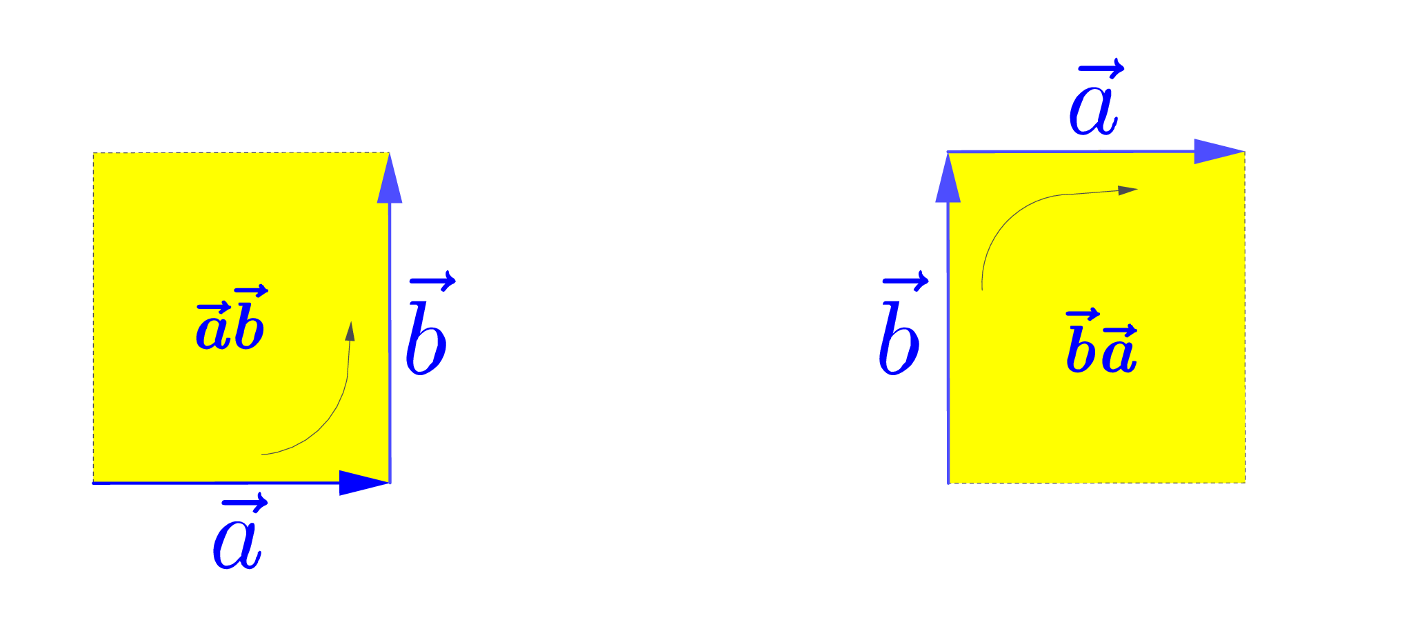
For the orthogonal vectors 𝐚\mathbf{a} and 𝐛\mathbf{b}, let us go further and give the new quantity 𝐁:=𝐚𝐛\mathbf{B}:=\mathbf{a}\mathbf{b} the geometric interpretation of a directed plane segment, or bivector, having the direction of the plane in which the vectors lies. The bivectors 𝐁\mathbf{B}, and its additive inverse 𝐛𝐚=−𝐚𝐛=−𝐁\mathbf{b}\mathbf{a}=-\mathbf{a}\mathbf{b}=-\mathbf{B}, are pictured in Figure 4. Just as the orientation of a vector is the determined by the direction of the line segment, the orientations of the bivectors 𝐁=𝐚𝐛\mathbf{B}=\mathbf{a}\mathbf{b} and −𝐁=𝐛𝐚-\mathbf{B}=\mathbf{b}\mathbf{a} are determined by the orientation of its sides, as shown in the Figure 4.

Refer to caption
Figure 4: The bivectors 𝐚𝐛\mathbf{a}\mathbf{b} and 𝐛𝐚\mathbf{b}\mathbf{a} defined by the orthogonal vectors 𝐚\mathbf{a} and 𝐛\mathbf{b}.

We have seen that a vector 𝐯=|𝐯|​𝐯^\mathbf{v}=|\mathbf{v}|\hat{\mathbf{v}} has the unit direction 𝐯^\hat{\mathbf{v}} and length |𝐯||\mathbf{v}|, and that 𝐯2=|𝐯|2\mathbf{v}^{2}=|\mathbf{v}|^{2}. Squaring the bivector 𝐁=𝐚𝐛\mathbf{B}=\mathbf{a}\mathbf{b} gives

𝐁2=(𝐚𝐛)​(𝐚𝐛)=−𝐚𝐛𝐛𝐚=−𝐚2​𝐛2=−|𝐚|2​|𝐛|2=−|𝐁|2,\mathbf{B}^{2}=(\mathbf{a}\mathbf{b})(\mathbf{a}\mathbf{b})=-\mathbf{a}\mathbf{b}\mathbf{b}\mathbf{a}=-\mathbf{a}^{2}\mathbf{b}^{2}=-|\mathbf{a}|^{2}|\mathbf{b}|^{2}=-|\mathbf{B}|^{2}, (5)

which is the negative of the area squared of the rectangle with the sides defined by the orthogonal vectors 𝐚\mathbf{a} and 𝐛\mathbf{b}. It follows that

𝐁=|𝐁|​𝐁^,\mathbf{B}=|\mathbf{B}|\hat{\mathbf{B}}, (6)

where |𝐁|=|𝐚|​|𝐛||\mathbf{B}|=|\mathbf{a}||\mathbf{b}| is the area of the directed plane segment, and its direction is the unit bivector 𝐁^=𝐚^​𝐛^\hat{\mathbf{B}}=\hat{\mathbf{a}}\hat{\mathbf{b}}, with

𝐁^2=(𝐚^​𝐛^)​(𝐚^​𝐛^)=𝐚^​(𝐛^​𝐚^)​𝐛^=−𝐚^2​𝐛^2=−1.\hat{\mathbf{B}}^{2}=(\hat{\mathbf{a}}\hat{\mathbf{b}})(\hat{\mathbf{a}}\hat{\mathbf{b}})=\hat{\mathbf{a}}(\hat{\mathbf{b}}\hat{\mathbf{a}})\hat{\mathbf{b}}=-\hat{\mathbf{a}}^{2}\hat{\mathbf{b}}^{2}=-1.

2.1 The inner product

Consider now the general triangle in Figure 5, with the vectors 𝐚\mathbf{a}, 𝐛\mathbf{b}, 𝐜\mathbf{c} along its sides satisfying the vector equation 𝐚+𝐛=𝐜\mathbf{a}+\mathbf{b}=\mathbf{c}. Squaring this equation gives

Refer to caption
Figure 5: Law of Cosines.
(𝐚+𝐛)2=𝐚2+𝐚𝐛+𝐛𝐚+𝐛2=𝐜2⇔|𝐚|2+2𝐚⋅𝐛+|𝐛|2=|𝐜|2,(\mathbf{a}+\mathbf{b})^{2}=\mathbf{a}^{2}+\mathbf{a}\mathbf{b}+\mathbf{b}\mathbf{a}+\mathbf{b}^{2}=\mathbf{c}^{2}\ \ \iff\ \ |\mathbf{a}|^{2}+2\mathbf{a}\cdot\mathbf{b}+|\mathbf{b}|^{2}=|\mathbf{c}|^{2},

known as the Law of Cosines, where

𝐚⋅𝐛:=12​(𝐚𝐛+𝐛𝐚)=|𝐚|​|𝐛|​cos⁡θ,\mathbf{a}\cdot\mathbf{b}:=\frac{1}{2}(\mathbf{a}\mathbf{b}+\mathbf{b}\mathbf{a})=|\mathbf{a}||\mathbf{b}|\cos\theta, (7)

is the inner product or dot product of the vectors 𝐚\mathbf{a} and 𝐛\mathbf{b}. In Figure 5, the angle −π≤θ≤π-\pi\leq\theta\leq\pi is measured from the vector 𝐚\mathbf{a} to the vector 𝐛\mathbf{b}, and

cos⁡θ=−cos⁡(π−θ)=−cos⁡C=cos⁡(−θ),\cos\theta=-\cos(\pi-\theta)=-\cos C=\cos(-\theta),

so the sign of the angle is unimportant. Note that (7) allows us to reverse the order of the geometric product,

𝐛𝐚=−𝐚𝐛+2​𝐚⋅𝐛.\mathbf{b}\mathbf{a}=-\mathbf{a}\mathbf{b}+2\mathbf{a}\cdot\mathbf{b}. (8)

We have used the usual rules for the multiplication of real numbers, except that we have not assumed that the multiplication of vectors is universally commutative. Indeed, the Pythagorean Theorem tells us that |𝐚|2+|𝐛|2=|𝐜|2|\mathbf{a}|^{2}+|\mathbf{b}|^{2}=|\mathbf{c}|^{2} only for a right triangle when 𝐚⋅𝐛=0\mathbf{a}\cdot\mathbf{b}=0, or equivalently, when the vectors 𝐚\mathbf{a} and 𝐛\mathbf{b} are orthogonal and anti-commute.

Now is a good place to summarize the rules which we have developed for the geometric multiplication of vectors. For vectors 𝐚\mathbf{a}, 𝐛\mathbf{b}, and 𝐜\mathbf{c},

  1. (P1)

    𝐚2=|𝐚|2\mathbf{a}^{2}=|\mathbf{a}|^{2}  The square of a vector is its magnitude squared

  2. (P2)

    𝐚𝐛=−𝐛𝐚\mathbf{a}\mathbf{b}=-\mathbf{b}\mathbf{a}  defines the bivector 𝐁=𝐚𝐛\mathbf{B}=\mathbf{a}\mathbf{b} when 𝐚\mathbf{a} and 𝐛\mathbf{b} are orthogonal vectors.

  3. (P3)

    𝐚⁡(𝐛+𝐜)=𝐚𝐛+𝐚𝐜\mathbf{a}(\mathbf{b}+\mathbf{c})=\mathbf{a}\mathbf{b}+\mathbf{a}\mathbf{c}  Left distributivity

  4. (P4)

    (𝐛+𝐜)​𝐚=𝐛𝐚+𝐜𝐚(\mathbf{b}+\mathbf{c})\mathbf{a}=\mathbf{b}\mathbf{a}+\mathbf{c}\mathbf{a}  Right distributivity

  5. (P5)

    𝐚⁡(𝐛𝐜)=(𝐚𝐛)​𝐜=𝐚𝐛𝐜\mathbf{a}(\mathbf{b}\mathbf{c})=(\mathbf{a}\mathbf{b})\mathbf{c}=\mathbf{a}\mathbf{b}\mathbf{c}  Product associativity

  6. (P6)

    0​𝐚=0=𝐚​00\mathbf{a}=0=\mathbf{a}0  Multiplication of a vector by zero is zero

  7. (P7)

    α​𝐚=𝐚​α,forα∈ℝ\alpha\mathbf{a}=\mathbf{a}\alpha,\ \ {\rm for}\ \ \alpha\in\mathbb{R}  Multiplication of a vector times a scalar is commutative

2.2 The outer product

So far, all is well, fine and good. The inner product of two vectors has been identified as one half the symmetric product of those vectors. To discover the geometric interpretation of the anti-symmetric product of the two vectors 𝐚\mathbf{a} and 𝐛\mathbf{b}, we write

𝐚𝐛=12​(𝐚𝐛+𝐛𝐚)+12​(𝐚𝐛−𝐛𝐚)=𝐚⋅𝐛+𝐚∧𝐛,\mathbf{a}\mathbf{b}=\frac{1}{2}(\mathbf{a}\mathbf{b}+\mathbf{b}\mathbf{a})+\frac{1}{2}(\mathbf{a}\mathbf{b}-\mathbf{b}\mathbf{a})=\mathbf{a}\cdot\mathbf{b}+\mathbf{a}\wedge\mathbf{b}, (9)

where 𝐚∧𝐛:=12​(𝐚𝐛−𝐛𝐚)\mathbf{a}\wedge\mathbf{b}:=\frac{1}{2}(\mathbf{a}\mathbf{b}-\mathbf{b}\mathbf{a}) is called the outer product, or wedge product between 𝐚\mathbf{a} and 𝐛\mathbf{b}. The outer product is antisymmetric, since 𝐛∧𝐚=−𝐚∧𝐛\mathbf{b}\wedge\mathbf{a}=-\mathbf{a}\wedge\mathbf{b}. Indeed, when 𝐚⋅𝐛=0\mathbf{a}\cdot\mathbf{b}=0 the geometric product reduces to the outer product, i.e.

𝐚𝐛=𝐚⋅𝐛+𝐚∧𝐛=𝐚∧𝐛=−𝐛𝐚.\mathbf{a}\mathbf{b}=\mathbf{a}\cdot\mathbf{b}+\mathbf{a}\wedge\mathbf{b}=\mathbf{a}\wedge\mathbf{b}=-\mathbf{b}\mathbf{a}. (10)

It is natural to give 𝐚∧𝐛\mathbf{a}\wedge\mathbf{b} the interpretation of a directed plane segment or bivector. To see this, write 𝐛=𝐛∥+𝐛⟂\mathbf{b}=\mathbf{b}_{\parallel}+\mathbf{b}_{\perp}, where 𝐛∥=s​𝐚\mathbf{b}_{\parallel}=s\mathbf{a}, for s∈ℝs\in\mathbb{R}, is the vector part of 𝐛\mathbf{b} which is parallel to 𝐚\mathbf{a}, and 𝐛⟂\mathbf{b}_{\perp} is the vector part of 𝐛\mathbf{b} which is perpendicular to 𝐚\mathbf{a}. Calculating 𝐚𝐛\mathbf{a}\mathbf{b}, we find

𝐚𝐛=𝐚⁡(𝐛∥+𝐛⟂)=𝐚𝐛∥+𝐚𝐛⟂=s​𝐚2+𝐚𝐛⟂=𝐚⋅𝐛+𝐚∧𝐛.\mathbf{a}\mathbf{b}=\mathbf{a}(\mathbf{b}_{\parallel}+\mathbf{b}_{\perp})=\mathbf{a}\mathbf{b}_{\parallel}+\mathbf{a}\mathbf{b}_{\perp}=s\mathbf{a}^{2}+\mathbf{a}\mathbf{b}_{\perp}=\mathbf{a}\cdot\mathbf{b}+\mathbf{a}\wedge\mathbf{b}.

Equating scalar and bivector parts, gives

𝐚⋅𝐛=s​𝐚2and𝐚∧𝐛=𝐚𝐛⟂.\mathbf{a}\cdot\mathbf{b}=s\mathbf{a}^{2}\quad{\rm and}\quad\mathbf{a}\wedge\mathbf{b}=\mathbf{a}\mathbf{b}_{\perp}. (11)

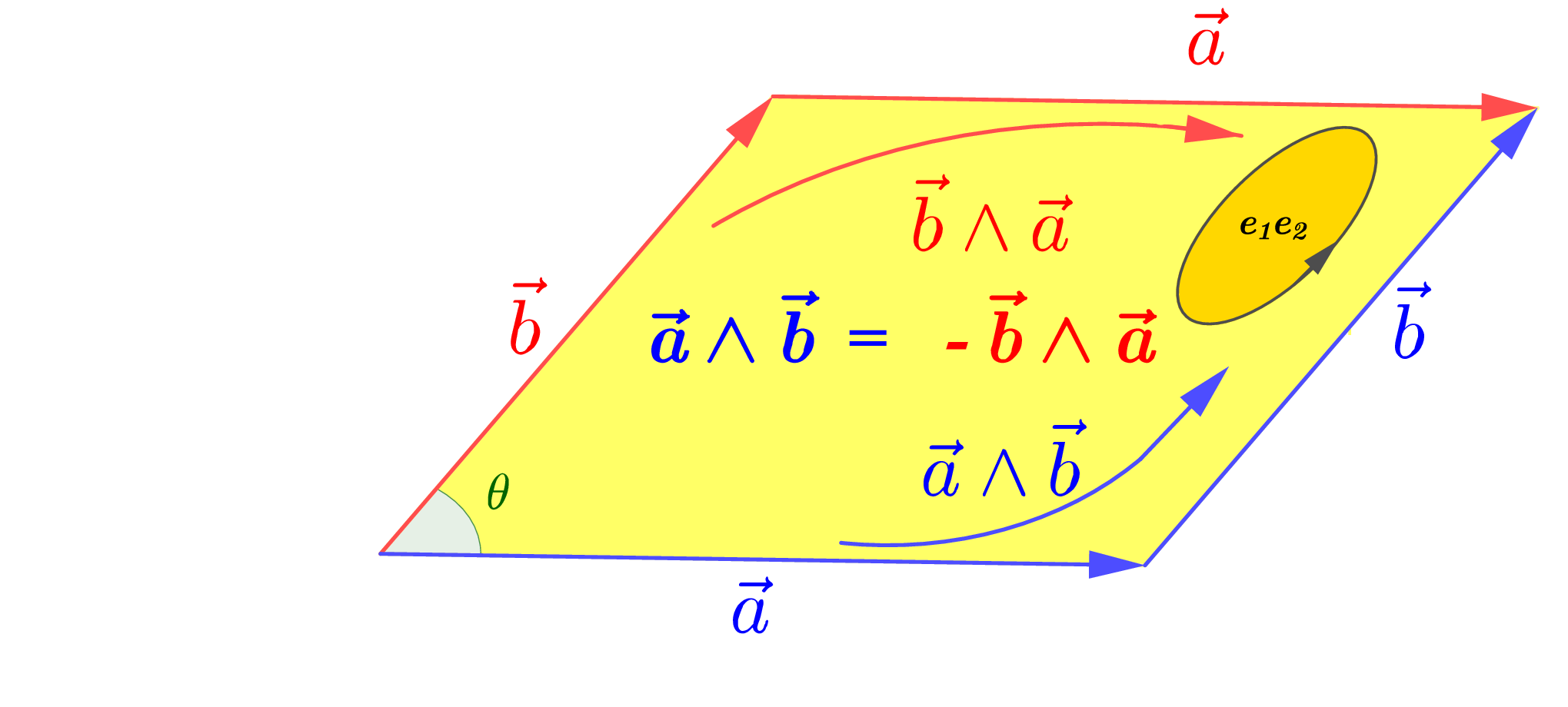
It follows that 𝐚∧𝐛=𝐚𝐛⟂\mathbf{a}\wedge\mathbf{b}=\mathbf{a}\mathbf{b}_{\perp} is the bivector which is the product of the orthogonal vectors 𝐚\mathbf{a} and 𝐛⟂\mathbf{b}_{\perp}, shown in Figure 5. The bivector defined by the oriented parallelogram 𝐚∧𝐛\mathbf{a}\wedge\mathbf{b}, with sides 𝐚\mathbf{a} and 𝐛\mathbf{b}, has exactly the same orientation and directed area as the bivector defined by the oriented rectangle 𝐚𝐛⟂\mathbf{a}\mathbf{b}_{\perp}, with the sides 𝐚\mathbf{a} and 𝐛⟂\mathbf{b}_{\perp}.

Refer to caption
Figure 6: Orientation of a bivector. The area, or magnitude of the bivector 𝐚∧𝐛\mathbf{a}\wedge\mathbf{b} is |𝐚∧𝐛|=|𝐚|​|𝐛|​|sin⁡θ||\mathbf{a}\wedge\mathbf{b}|=|\mathbf{a}||\mathbf{b}||\sin\theta|, where −π≤θ<π-\pi\leq\theta<\pi, and its direction is the unit bivector 𝐞1​𝐞2\mathbf{e}_{1}\mathbf{e}_{2}. Note that the shape of the bivector 𝐞12:=𝐞1​𝐞2\mathbf{e}_{12}:=\mathbf{e}_{1}\mathbf{e}_{2} is unimportant, only the plane in which it lies and its orientation.

We have seen that the square of a vector is its magnitude squared, 𝐚2=|𝐚|2\mathbf{a}^{2}=|\mathbf{a}|^{2}. What about the square of the bivector (𝐚∧𝐛)(\mathbf{a}\wedge\mathbf{b})? Using (11), we find that

(𝐚∧𝐛)2=(𝐚𝐛⟂)2=−𝐚2​𝐛⟂2=−|𝐚∧𝐛|2,(\mathbf{a}\wedge\mathbf{b})^{2}=(\mathbf{a}\mathbf{b}_{\perp})^{2}=-\mathbf{a}^{2}\mathbf{b}_{\perp}^{2}=-|\mathbf{a}\wedge\mathbf{b}|^{2}, (12)

in agreement with (5). If the bivector is in the x​yxy-plane of the unit bivector 𝐞1​𝐞2\mathbf{e}_{1}\mathbf{e}_{2}, where the unit vectors 𝐞1\mathbf{e}_{1} and 𝐞2\mathbf{e}_{2} lie along the orthogonal xx- and yy-axes, respectively, then 𝐚∧𝐛=𝐞12​|𝐚|​|𝐛|​sin⁡θ\mathbf{a}\wedge\mathbf{b}=\mathbf{e}_{12}|\mathbf{a}||\mathbf{b}|\sin\theta, see Figure 6. The geometric product in ℝ2\mathbb{R}^{2} and ℝ3\mathbb{R}^{3} is further discussed in Section 3.

Refer to caption
Figure 7: The wedge product is distributive over the addition of vectors.

Just as sum of vectors is a vector, the sum of bivectors is a bivector. Figure 7 shows the sum of the bivectors

𝐚∧𝐜+𝐛∧𝐜=(𝐚+𝐛)∧𝐜,\mathbf{a}\wedge\mathbf{c}+\mathbf{b}\wedge\mathbf{c}=(\mathbf{a}+\mathbf{b})\wedge\mathbf{c},

and also shows the distributive property of the outer product over the sum of the vectors 𝐚\mathbf{a} and 𝐛\mathbf{b}.

2.3 Properties of the inner and outer products

Since the triangle in Figure 5 satisfies the vector equation

𝐚+𝐛=𝐜,\mathbf{a}+\mathbf{b}=\mathbf{c},

by wedging both sides of this equation by 𝐚,𝐛\mathbf{a},\mathbf{b} and 𝐜\mathbf{c}, gives

𝐚∧𝐛=𝐜∧𝐛,𝐛∧𝐚=𝐜∧𝐚,and𝐜∧𝐚=𝐛∧𝐜,\mathbf{a}\wedge\mathbf{b}=\mathbf{c}\wedge\mathbf{b},\ \ \mathbf{b}\wedge\mathbf{a}=\mathbf{c}\wedge\mathbf{a},\ \ {\rm and}\ \ \mathbf{c}\wedge\mathbf{a}=\mathbf{b}\wedge\mathbf{c},

or equivalently,

𝐚∧𝐛=𝐜∧𝐛=𝐚∧𝐜.\mathbf{a}\wedge\mathbf{b}=\mathbf{c}\wedge\mathbf{b}=\mathbf{a}\wedge\mathbf{c}.

Note that the area of the triangle is given by 12​|𝐚∧𝐛|\frac{1}{2}|\mathbf{a}\wedge\mathbf{b}|, which is one half of the area of the parallelogram 𝐚∧𝐛\mathbf{a}\wedge\mathbf{b}, so the last equation is reflecting the equivalent relationship between parallelograms.

Dividing each term of the last equality by |𝐚​‖𝐛‖​𝐜||\mathbf{a}||\mathbf{b}||\mathbf{c}|, gives

𝐚^∧𝐛^|𝐜|=𝐜^∧𝐛^|𝐚|=𝐚^∧𝐜^|𝐛|⟹|𝐚^∧𝐛^||𝐜|=|𝐜^∧𝐛^||𝐚|=|𝐚^∧𝐜^||𝐛|.\frac{\hat{\mathbf{a}}\wedge\hat{\mathbf{b}}}{|\mathbf{c}|}=\frac{\hat{\mathbf{c}}\wedge\hat{\mathbf{b}}}{|\mathbf{a}|}=\frac{\hat{\mathbf{a}}\wedge\hat{\mathbf{c}}}{|\mathbf{b}|}\ \ \Longrightarrow\frac{|\hat{\mathbf{a}}\wedge\hat{\mathbf{b}}|}{|\mathbf{c}|}=\frac{|\hat{\mathbf{c}}\wedge\hat{\mathbf{b}}|}{|\mathbf{a}|}=\frac{|\hat{\mathbf{a}}\wedge\hat{\mathbf{c}}|}{|\mathbf{b}|}.

For the angles 0≤A,B,C≤π0\leq A,B,C\leq\pi,

|𝐚^∧𝐛^|=sinC=sin(π−C),|𝐜^∧𝐛^|=sinA,and|𝐚^∧𝐜^|=sinB,|\hat{\mathbf{a}}\wedge\hat{\mathbf{b}}|=\sin C=\sin(\pi-C),\ \ |\hat{\mathbf{c}}\wedge\hat{\mathbf{b}}|=\sin A,\ \ {\rm and}\ \ |\hat{\mathbf{a}}\wedge\hat{\mathbf{c}}|=\sin B,

from which it follows that

sin⁡A|𝐚|=sin⁡B|𝐛|=sin⁡C|𝐜|\frac{\sin A}{|\mathbf{a}|}=\frac{\sin B}{|\mathbf{b}|}=\frac{\sin C}{|\mathbf{c}|}

known as the Law of Sines, see Figure 8.

Refer to caption
Figure 8: Law of Sines.

In (9), we discovered that the geometric product of two vectors splits into two parts, a symmetric scalar part 𝐚⋅𝐛\mathbf{a}\cdot\mathbf{b} and an anti-symmetric bivector part 𝐚∧𝐛\mathbf{a}\wedge\mathbf{b}. It is natural to ask the question whether the geometric product of a vector 𝐚\mathbf{a} with a bivector 𝐛∧𝐜\mathbf{b}\wedge\mathbf{c} has a similar decomposition? Analogous to (9), we write

𝐚⁡(𝐛∧𝐜)=𝐚⋅(𝐛∧𝐜)+𝐚∧(𝐛∧𝐜),\mathbf{a}(\mathbf{b}\wedge\mathbf{c})=\mathbf{a}\cdot(\mathbf{b}\wedge\mathbf{c})+\mathbf{a}\wedge(\mathbf{b}\wedge\mathbf{c}), (13)

where in this case

𝐚⋅(𝐛∧𝐜):=12(𝐚(𝐛∧𝐜)−(𝐛∧𝐜)𝐚)=:−(𝐛∧𝐜)⋅𝐚\mathbf{a}\cdot(\mathbf{b}\wedge\mathbf{c}):=\frac{1}{2}\Big(\mathbf{a}(\mathbf{b}\wedge\mathbf{c})-(\mathbf{b}\wedge\mathbf{c})\mathbf{a}\Big)=:-(\mathbf{b}\wedge\mathbf{c})\cdot\mathbf{a} (14)

is antisymmetric, and

𝐚∧(𝐛∧𝐜):=12​(𝐚⁡(𝐛∧𝐜)+(𝐛∧𝐜)​𝐚)=:(𝐛∧𝐜)∧𝐚\mathbf{a}\wedge(\mathbf{b}\wedge\mathbf{c}):=\frac{1}{2}\Big(\mathbf{a}(\mathbf{b}\wedge\mathbf{c})+(\mathbf{b}\wedge\mathbf{c})\mathbf{a}\Big)=:(\mathbf{b}\wedge\mathbf{c})\wedge\mathbf{a} (15)

is symmetric.

To better understand this decomposition, we consider each part separately. Starting with 𝐚⋅(𝐛∧𝐜)=𝐚∥​(𝐛∧𝐜)\mathbf{a}\cdot(\mathbf{b}\wedge\mathbf{c})=\mathbf{a}_{\parallel}(\mathbf{b}\wedge\mathbf{c}), we first show that

𝐚⋅(𝐛∧𝐜)=(𝐚⋅𝐛)​𝐜−(𝐚⋅𝐜)​𝐛.\mathbf{a}\cdot(\mathbf{b}\wedge\mathbf{c})=(\mathbf{a}\cdot\mathbf{b})\mathbf{c}-(\mathbf{a}\cdot\mathbf{c})\mathbf{b}. (16)

Decomposing the left side of this equation, using (14) and (9), gives

𝐚⋅(𝐛∧𝐜)=12​(𝐚⁡(𝐛∧𝐜)−(𝐛∧𝐜)​𝐚)=14​(𝐚𝐛𝐜−𝐚𝐜𝐛−𝐛𝐜𝐚+𝐜𝐛𝐚).\mathbf{a}\cdot(\mathbf{b}\wedge\mathbf{c})=\frac{1}{2}\Big(\mathbf{a}(\mathbf{b}\wedge\mathbf{c})-(\mathbf{b}\wedge\mathbf{c})\mathbf{a}\Big)=\frac{1}{4}(\mathbf{a}\mathbf{b}\mathbf{c}-\mathbf{a}\mathbf{c}\mathbf{b}-\mathbf{b}\mathbf{c}\mathbf{a}+\mathbf{c}\mathbf{b}\mathbf{a}).

Decomposing the right side, gives

(𝐚⋅𝐛)​𝐜−(𝐚⋅𝐜)​𝐛=12​((𝐚⋅𝐛)​𝐜+𝐜⁡(𝐚⋅𝐛)−(𝐚⋅𝐜)​𝐛−𝐛⁡(𝐚⋅𝐜))(\mathbf{a}\cdot\mathbf{b})\mathbf{c}-(\mathbf{a}\cdot\mathbf{c})\mathbf{b}=\frac{1}{2}\Big((\mathbf{a}\cdot\mathbf{b})\mathbf{c}+\mathbf{c}(\mathbf{a}\cdot\mathbf{b})-(\mathbf{a}\cdot\mathbf{c})\mathbf{b}-\mathbf{b}(\mathbf{a}\cdot\mathbf{c})\Big)
=14​((𝐚𝐛+𝐛𝐚)​𝐜+𝐜⁡(𝐚𝐛+𝐛𝐚)−(𝐚𝐜+𝐜𝐚)​𝐛−𝐛⁡(𝐚𝐜+𝐜𝐚))=\frac{1}{4}\Big((\mathbf{a}\mathbf{b}+\mathbf{b}\mathbf{a})\mathbf{c}+\mathbf{c}(\mathbf{a}\mathbf{b}+\mathbf{b}\mathbf{a})-(\mathbf{a}\mathbf{c}+\mathbf{c}\mathbf{a})\mathbf{b}-\mathbf{b}(\mathbf{a}\mathbf{c}+\mathbf{c}\mathbf{a})\Big)
=14​(𝐚𝐛𝐜−𝐚𝐜𝐛−𝐛𝐜𝐚+𝐜𝐛𝐚),=\frac{1}{4}(\mathbf{a}\mathbf{b}\mathbf{c}-\mathbf{a}\mathbf{c}\mathbf{b}-\mathbf{b}\mathbf{c}\mathbf{a}+\mathbf{c}\mathbf{b}\mathbf{a}),

which is in agreement with the left side. The geometric interpretation of (14) is given in the Figure 9.

Refer to caption
Figure 9: The result 𝐚⋅(𝐛∧𝐜){\mathbf{a}}\cdot({\mathbf{b}}\wedge{\mathbf{c}}) is the vector 𝐚\mathbf{a} projected onto the plane of 𝐛∧𝐜\mathbf{b}\wedge\mathbf{c}, and then rotated through 9090 degrees in this plane.

Regarding the triple wedge product (15), we need to show the associative property, 𝐚∧(𝐛∧𝐜)=(𝐚∧𝐛)∧𝐜\mathbf{a}\wedge(\mathbf{b}\wedge\mathbf{c})=(\mathbf{a}\wedge\mathbf{b})\wedge\mathbf{c}. Decomposing both sides of this equation, using (10) and (15), gives

𝐚∧(𝐛∧𝐜):=12​(𝐚⁡(𝐛∧𝐜)+(𝐛∧𝐜)​𝐚)=14​(𝐚⁡(𝐛𝐜−𝐜𝐛)+(𝐛𝐜−𝐜𝐛)​𝐚),\mathbf{a}\wedge(\mathbf{b}\wedge\mathbf{c}):=\frac{1}{2}\Big(\mathbf{a}(\mathbf{b}\wedge\mathbf{c})+(\mathbf{b}\wedge\mathbf{c})\mathbf{a}\Big)=\frac{1}{4}\Big(\mathbf{a}(\mathbf{b}\mathbf{c}-\mathbf{c}\mathbf{b})+(\mathbf{b}\mathbf{c}-\mathbf{c}\mathbf{b})\mathbf{a}\Big),

and

(𝐚∧𝐛)∧𝐜:=12​((𝐚∧𝐛)​𝐜+𝐜⁡(𝐚∧𝐛))=14​((𝐚𝐛−𝐛𝐚)​𝐜+𝐜⁡(𝐚𝐛−𝐛𝐚)).(\mathbf{a}\wedge\mathbf{b})\wedge\mathbf{c}:=\frac{1}{2}\Big((\mathbf{a}\wedge\mathbf{b})\mathbf{c}+\mathbf{c}(\mathbf{a}\wedge\mathbf{b})\Big)=\frac{1}{4}\Big((\mathbf{a}\mathbf{b}-\mathbf{b}\mathbf{a})\mathbf{c}+\mathbf{c}(\mathbf{a}\mathbf{b}-\mathbf{b}\mathbf{a})\Big).

To finish the argument, we have

𝐚∧(𝐛∧𝐜)−(𝐚∧𝐛)∧𝐜=14​(−𝐚𝐜𝐛−𝐜𝐚𝐛+𝐛𝐜𝐚+𝐛𝐚𝐜)\mathbf{a}\wedge(\mathbf{b}\wedge\mathbf{c})-(\mathbf{a}\wedge\mathbf{b})\wedge\mathbf{c}=\frac{1}{4}\Big(-\mathbf{a}\mathbf{c}\mathbf{b}-\mathbf{c}\mathbf{a}\mathbf{b}+\mathbf{b}\mathbf{c}\mathbf{a}+\mathbf{b}\mathbf{a}\mathbf{c}\Big)
=12​(−(𝐚⋅𝐜)​𝐛+𝐛⁡(𝐚⋅𝐜))=0.=\frac{1}{2}\Big(-(\mathbf{a}\cdot\mathbf{c})\mathbf{b}+\mathbf{b}(\mathbf{a}\cdot\mathbf{c})\Big)=0.

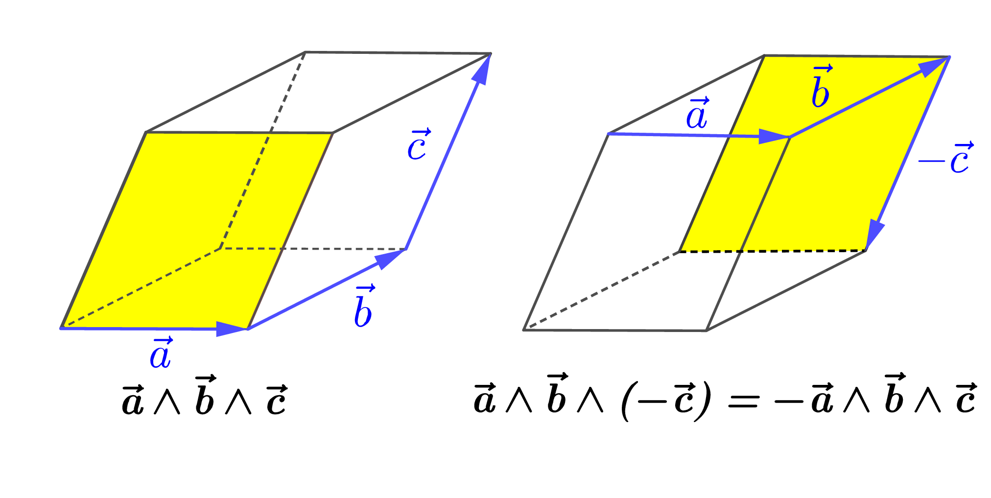
The trivector or directed volume 𝐚∧𝐛∧𝐜\mathbf{a}\wedge\mathbf{b}\wedge\mathbf{c} is pictured in Figure 10. There are many more similar identities in higher dimensional geometric algebras [7, 11].

Refer to caption
Figure 10: The sign of the vector 𝐜\mathbf{c} determines the right and left handed orientation of the trivector 𝐚∧𝐛∧𝐜\mathbf{a}\wedge\mathbf{b}\wedge\mathbf{c} shown.

Exercise: Using the properties (15) and (16), prove the Associative Law (P5) for the geometric product of vectors,

𝐚⁡(𝐛𝐜)=(𝐚𝐛)​𝐜.\mathbf{a}(\mathbf{b}\mathbf{c})=(\mathbf{a}\mathbf{b})\mathbf{c}.

3 The geometric algebras 𝔾1\mathbb{G}_{1}, 𝔾2\mathbb{G}_{2} and 𝔾3\mathbb{G}_{3}.

In the previous section, we discovered two general principals for the multiplication of Euclidean vectors 𝐚\mathbf{a} and 𝐛\mathbf{b}:

  • 1)

    The square of a vector is its length squared, 𝐚2=|𝐚|2\mathbf{a}^{2}=|\mathbf{a}|^{2}.

  • 2)

    If the vectors 𝐚\mathbf{a} and 𝐛\mathbf{b} are orthogonal to each other, i.e., the angle between them is 9090 degrees, then they anti-commute 𝐚𝐛=−𝐛𝐚\mathbf{a}\mathbf{b}=-\mathbf{b}\mathbf{a} and define the bivector given in (6).

These two general rules hold for Euclidean vectors, independent of the dimension of the space in which they lie.

The simplest euclidean geometric algebra is obtained by extending the real number system ℝ\mathbb{R} to include a single new square root of +1+1, giving the geometric algebra

𝔾1:=ℝ⁡(𝐞),\mathbb{G}_{1}:=\mathbb{R}(\mathbf{e}),

where 𝐞2=1\mathbf{e}^{2}=1. A geometric number in 𝔾1\mathbb{G}_{1} has the form

g=x+y​𝐞,g=x+y\mathbf{e},

where x,y∈ℝx,y\in\mathbb{R}, and defines the hyperbolic number plane [9].

We now apply what we have learned about the general geometric addition and multiplication of vectors to vectors in the two dimensional plane ℝ2\mathbb{R}^{2}, and in the three dimensional space ℝ3\mathbb{R}^{3} of experience. The 22-dimensional coordinate plane is defined by

ℝ2:={(x,y)|x,y∈ℝ}.\mathbb{R}^{2}:=\{(x,y)|\ \ x,y\in\mathbb{R}\}. (17)

By laying out two orthonormal unit vectors {𝐞1,𝐞2}\{\mathbf{e}_{1},\mathbf{e}_{2}\} along the xx- and yy-axes, respectively, each point

(x,y)∈ℝ2⟷𝐱=x𝐞1+y𝐞2∈ℝ2(x,y)\in\mathbb{R}^{2}\quad\longleftrightarrow\quad\mathbf{x}=x\mathbf{e}_{1}+y\mathbf{e}_{2}\in\mathbb{R}^{2} (18)

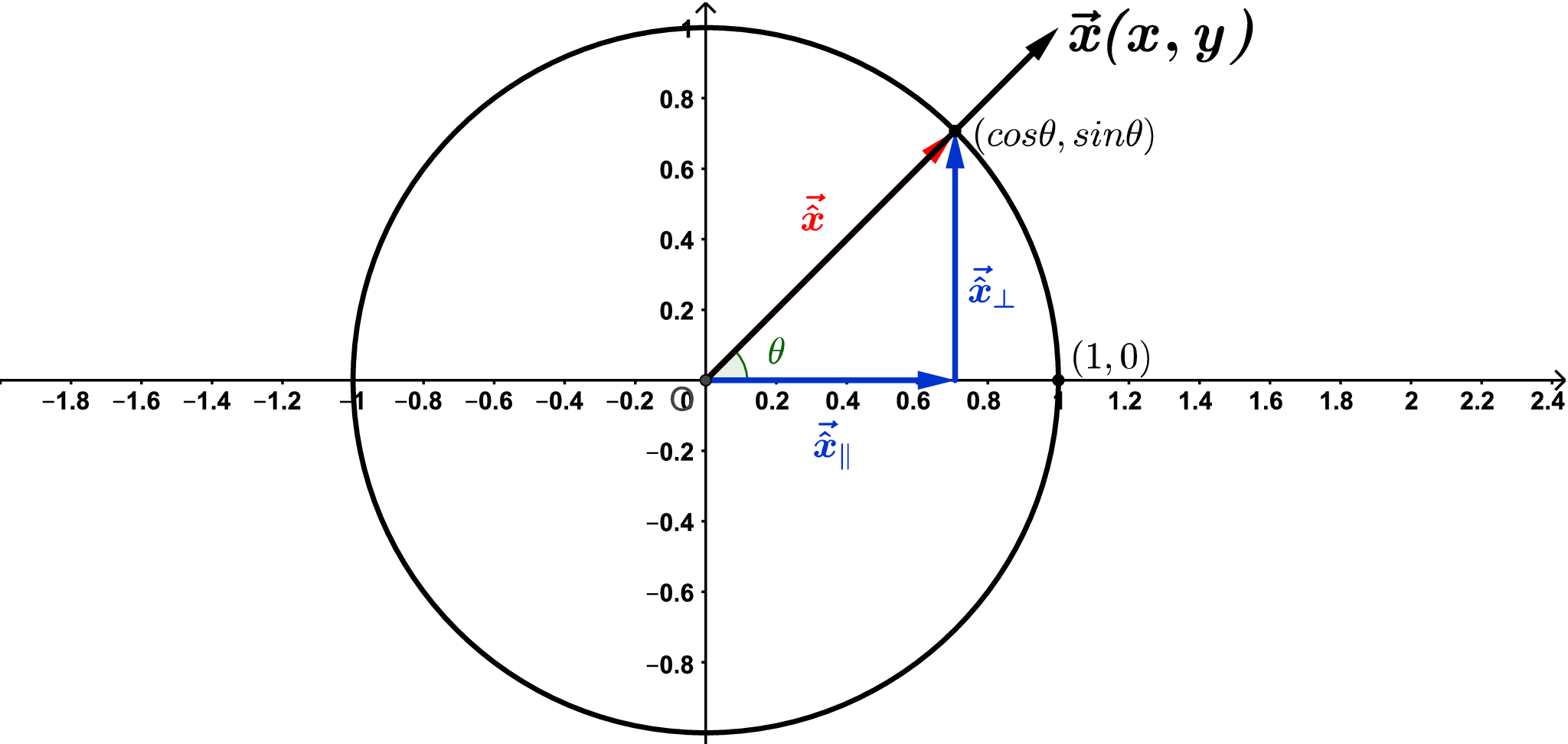
becomes a position vector 𝐱=|𝐱|​𝐱^\mathbf{x}=|\mathbf{x}|\hat{\mathbf{x}} from the origin, shown in Figure 11 with the unit circle. The point 𝐱^=(cos⁡θ,sin⁡θ)\hat{\mathbf{x}}=(\cos\theta,\sin\theta) on the unit circle S1S^{1}, where the angle θ\theta is measured from the xx-axis, becomes the unit vector

𝐱^=cos⁡(θ)​𝐞1+sin⁡(θ)​𝐞2.\hat{\mathbf{x}}=\cos(\theta)\mathbf{e}_{1}+\sin(\theta)\mathbf{e}_{2}.

In equation (18), we have abused notation by equating the coordinate point (x,y)∈ℝ2(x,y)\in\mathbb{R}^{2} with the position vector 𝐱=x​𝐞1+y​𝐞2\mathbf{x}=x\mathbf{e}_{1}+y\mathbf{e}_{2} from the origin of ℝ2\mathbb{R}^{2}.

Refer to caption
Figure 11: The unit circle S1S^{1} in the x​yxy-plane.

Calculating the geometric product of the two vectors

𝐚=(a1,a2)=a1​𝐞1+a2​𝐞2,𝐛=(b1,b2)=b1​𝐞1+b2​𝐞2,\mathbf{a}=(a_{1},a_{2})=a_{1}\mathbf{e}_{1}+a_{2}\mathbf{e}_{2},\quad\mathbf{b}=(b_{1},b_{2})=b_{1}\mathbf{e}_{1}+b_{2}\mathbf{e}_{2},

in the x​yxy-plane, we obtain

𝐚𝐛=(a1​𝐞1+a2​𝐞2)​(b1​𝐞1+b2​𝐞2)\mathbf{a}\mathbf{b}=(a_{1}\mathbf{e}_{1}+a_{2}\mathbf{e}_{2})(b_{1}\mathbf{e}_{1}+b_{2}\mathbf{e}_{2})
=a1​b1​𝐞12+a2​b2​𝐞22+a1​b2​𝐞1​𝐞2+a2​b1​𝐞2​𝐞1=a_{1}b_{1}\mathbf{e}_{1}^{2}+a_{2}b_{2}\mathbf{e}_{2}^{2}+a_{1}b_{2}\mathbf{e}_{1}\mathbf{e}_{2}+a_{2}b_{1}\mathbf{e}_{2}\mathbf{e}_{1}
=(a1​b1+a2​b2)+(a1​b2−a2​b1)​𝐞1​𝐞2=𝐚⋅𝐛+𝐚∧𝐛,=(a_{1}b_{1}+a_{2}b_{2})+(a_{1}b_{2}-a_{2}b_{1})\mathbf{e}_{1}\mathbf{e}_{2}=\mathbf{a}\cdot\mathbf{b}+\mathbf{a}\wedge\mathbf{b}, (19)

where the inner product 𝐚⋅𝐛=a1​b1+a2​b2=|𝐚|​|𝐛|​cos⁡θ\mathbf{a}\cdot\mathbf{b}=a_{1}b_{1}+a_{2}b_{2}=|\mathbf{a}||\mathbf{b}|\cos\theta, and the outer product

𝐚∧𝐛=(a1​b2−a2​b1)​𝐞12=𝐞12​|𝐚|​|𝐛|​sin⁡θ\mathbf{a}\wedge\mathbf{b}=(a_{1}b_{2}-a_{2}b_{1})\mathbf{e}_{12}=\mathbf{e}_{12}|\mathbf{a}||\mathbf{b}|\sin\theta

for 𝐞12:=𝐞1​𝐞2=𝐞1∧𝐞2\mathbf{e}_{12}:=\mathbf{e}_{1}\mathbf{e}_{2}=\mathbf{e}_{1}\wedge\mathbf{e}_{2}. The bivector 𝐚∧𝐛\mathbf{a}\wedge\mathbf{b} is pictured in Figure 12, together with a picture proof that the magnitude |𝐚∧𝐛|=|a1​b2−a2​b1||\mathbf{a}\wedge\mathbf{b}|=|a_{1}b_{2}-a_{2}b_{1}|, as expected.

Refer to caption
Figure 12: The outer product 𝐚∧𝐛\mathbf{a}\wedge\mathbf{b} in 2-dimensions.

By introducing the unit vectors {𝐞1,𝐞2}\{\mathbf{e}_{1},\mathbf{e}_{2}\} along the coordinate axes of ℝ2\mathbb{R}^{2}, and using properties of the geometric product, we have found explicit formulas for the dot and outer products of any two vectors 𝐚\mathbf{a} and 𝐛\mathbf{b} in ℝ2\mathbb{R}^{2}. The geometric product of the orthogonal unit vectors 𝐞1\mathbf{e}_{1} and 𝐞2\mathbf{e}_{2} gives the unit bivector 𝐞12\mathbf{e}_{12}, already pictured in Figure 6. Squaring 𝐞12\mathbf{e}_{12}, gives

𝐞122=(𝐞1​𝐞2)​(𝐞1​𝐞2)=−𝐞12​𝐞22=−1,\mathbf{e}_{12}^{2}=(\mathbf{e}_{1}\mathbf{e}_{2})(\mathbf{e}_{1}\mathbf{e}_{2})=-\mathbf{e}_{1}^{2}\mathbf{e}_{2}^{2}=-1,

which because of (5) and (12) is no surprise.

The most general geometric number of the 22-dimensional Euclidean plane ℝ2\mathbb{R}^{2} is

g=g0+g1​𝐞1+g2​𝐞2+g3​𝐞12,g=g_{0}+g_{1}\mathbf{e}_{1}+g_{2}\mathbf{e}_{2}+g_{3}\mathbf{e}_{12},

where gμ∈ℝg_{\mu}\in\mathbb{R} for μ=0,1,2,3\mu=0,1,2,3. The set of all geometric numbers gg, together with the two operations of geometric addition and multiplication, make up the geometric algebra 𝔾2\mathbb{G}_{2} of the Euclidean plane ℝ2\mathbb{R}^{2},

𝔾2:={g|g=g0+g1𝐞1+g2𝐞2+g3𝐞12}=ℝ(𝐞1,𝐞2).\mathbb{G}_{2}:=\{g|\ \ g=g_{0}+g_{1}\mathbf{e}_{1}+g_{2}\mathbf{e}_{2}+g_{3}\mathbf{e}_{12}\}=\mathbb{R}(\mathbf{e}_{1},\mathbf{e}_{2}).

The formal rules for the geometric addition and multiplication of the geometric numbers in 𝔾2\mathbb{G}_{2} are exactly the same as the rules for addition and multiplication of real numbers, except we give up universal commutativity to express the anti-commutativity of orthogonal vectors.

The geometric algebra 𝔾2\mathbb{G}_{2} breaks into two parts,

𝔾2=𝔾20+𝔾21+𝔾22=𝔾2++𝔾2−,\mathbb{G}_{2}=\mathbb{G}_{2}^{0}+\mathbb{G}_{2}^{1}+\mathbb{G}_{2}^{2}=\mathbb{G}_{2}^{+}+\mathbb{G}_{2}^{-},

where the even part, consisting of scalars (real numbers) and bivectors,

𝔾2+:=𝔾20+2={x+y𝐞12|x,y∈ℝ}=~ℂ\mathbb{G}_{2}^{+}:=\mathbb{G}_{2}^{0+2}=\{x+y\mathbf{e}_{12}|\ \ x,y\in\mathbb{R}\}\ \widetilde{=}\ \mathbb{C}

is algebraically closed and isomorphic to the complex number ℂ\mathbb{C}, and the odd part,

𝔾2−:=𝔾21={𝐱|𝐱=x𝐞1+y𝐞2}≡ℝ2\mathbb{G}_{2}^{-}:=\mathbb{G}_{2}^{1}=\{\mathbf{x}|\ \ \mathbf{x}=x\mathbf{e}_{1}+y\mathbf{e}_{2}\}\equiv\mathbb{R}^{2}

for x,y∈ℝx,y\in\mathbb{R}, consists of vectors in the x​yxy-plane ℝ2\mathbb{R}^{2}. The geometric algebra 𝔾2\mathbb{G}_{2} unites the vector plane 𝔾2−\mathbb{G}_{2}^{-} and the complex number plane 𝔾2+\mathbb{G}_{2}^{+} into a unified geometric number system 𝔾2\mathbb{G}_{2} of the plane.

By introducing a third unit vector 𝐞3\mathbf{e}_{3} into ℝ2\mathbb{R}^{2}, along the zz-axis, we get the 33-dimensional space ℝ3\mathbb{R}^{3}. All of the formulas found in ℝ2\mathbb{R}^{2} can then be extended to ℝ3\mathbb{R}^{3}, and by the same process, to any higher nn-dimensional space ℝn\mathbb{R}^{n} for n>3n>3. Geometric algebras can always be extended to higher dimensional geometric algebras simply by introducing additional orthogonal anti-commuting unit vectors with square ±1\pm 1, [14, 15].

Let us see how the formulas (19) work out explicitly in

ℝ3:={𝐱|𝐱=(x,y,z)=x𝐞1+y𝐞2+z𝐞3},\mathbb{R}^{3}:=\{\mathbf{x}|\quad\mathbf{x}=(x,y,z)=x\mathbf{e}_{1}+y\mathbf{e}_{2}+z\mathbf{e}_{3}\}, (20)

for x,y,z∈ℝx,y,z\in\mathbb{R}. For vectors

𝐚=a1​𝐞1+a2​𝐞2+a3​𝐞3,𝐛=b1​𝐞1+b2​𝐞2+b3​𝐞3,\mathbf{a}=a_{1}\mathbf{e}_{1}+a_{2}\mathbf{e}_{2}+a_{3}\mathbf{e}_{3},\quad\mathbf{b}=b_{1}\mathbf{e}_{1}+b_{2}\mathbf{e}_{2}+b_{3}\mathbf{e}_{3},

we calculate

𝐚𝐛=(a1​𝐞1+a2​𝐞2+a3​𝐞3)​(b1​𝐞1+b2​𝐞2+b3​𝐞3)\mathbf{a}\mathbf{b}=(a_{1}\mathbf{e}_{1}+a_{2}\mathbf{e}_{2}+a_{3}\mathbf{e}_{3})(b_{1}\mathbf{e}_{1}+b_{2}\mathbf{e}_{2}+b_{3}\mathbf{e}_{3})
=a1​b1​𝐞12+a2​b2​𝐞22+a3​b3​𝐞32=a_{1}b_{1}\mathbf{e}_{1}^{2}+a_{2}b_{2}\mathbf{e}_{2}^{2}+a_{3}b_{3}\mathbf{e}_{3}^{2}
+a1​b2​𝐞1​𝐞2+a2​b1​𝐞2​𝐞1+a2​b3​𝐞2​𝐞3+a3​b2​𝐞3​𝐞2+a1​b3​𝐞1​𝐞3+a3​b1​𝐞3​𝐞1+a_{1}b_{2}\mathbf{e}_{1}\mathbf{e}_{2}+a_{2}b_{1}\mathbf{e}_{2}\mathbf{e}_{1}+a_{2}b_{3}\mathbf{e}_{2}\mathbf{e}_{3}+a_{3}b_{2}\mathbf{e}_{3}\mathbf{e}_{2}+a_{1}b_{3}\mathbf{e}_{1}\mathbf{e}_{3}+a_{3}b_{1}\mathbf{e}_{3}\mathbf{e}_{1}
=(a1​b1+a2​b2+a3​b3)+(a1​b2−a2​b1)​𝐞12+(a2​b3−a3​b2)​𝐞23+(a1​b3−a3​b1)​𝐞13=(a_{1}b_{1}+a_{2}b_{2}+a_{3}b_{3})+(a_{1}b_{2}-a_{2}b_{1})\mathbf{e}_{12}+(a_{2}b_{3}-a_{3}b_{2})\mathbf{e}_{23}+(a_{1}b_{3}-a_{3}b_{1})\mathbf{e}_{13}

where the dot or inner product,

𝐚⋅𝐛=a1​b1+a2​b2+a3​b3=|𝐚|​|𝐛|​cos⁡θ,\mathbf{a}\cdot\mathbf{b}=a_{1}b_{1}+a_{2}b_{2}+a_{3}b_{3}=|\mathbf{a}||\mathbf{b}|\cos\theta,

and the outer product (11),

𝐚∧𝐛=(a1​b2−a2​b1)​𝐞12+(a2​b3−a3​b2)​𝐞23+(a1​b3−a3​b1)​𝐞13=|𝐚|​|𝐛|​𝐁^​sin⁡θ.\mathbf{a}\wedge\mathbf{b}=(a_{1}b_{2}-a_{2}b_{1})\mathbf{e}_{12}+(a_{2}b_{3}-a_{3}b_{2})\mathbf{e}_{23}+(a_{1}b_{3}-a_{3}b_{1})\mathbf{e}_{13}=|\mathbf{a}||\mathbf{b}|\hat{\mathbf{B}}\sin\theta. (21)

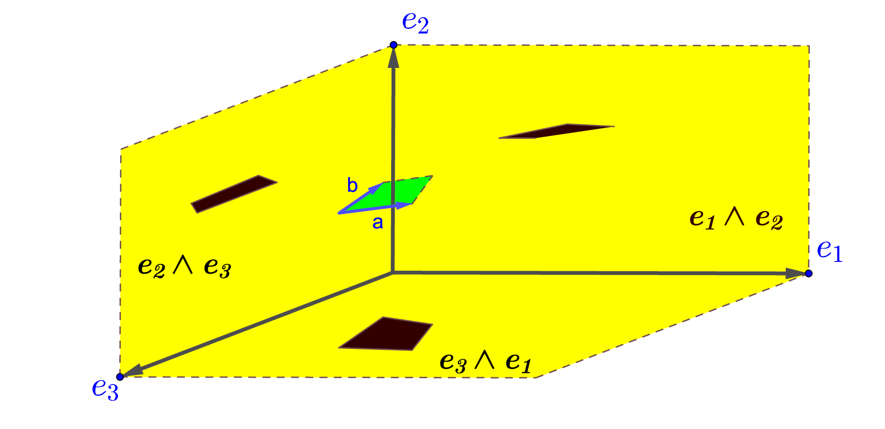
The sum of the three bivector components, which are projections onto the coordinate planes, are shown in Figure 13.

Refer to caption
Figure 13: Bivector decomposition in 3D space.

In ℝ3\mathbb{R}^{3}, the outer product 𝐚∧𝐛\mathbf{a}\wedge\mathbf{b} can be expressed in terms of the well known cross product of the century old, pre-Einstein Gibbs-Heaviside vector analysis. The vector cross product of the vectors 𝐚\mathbf{a} and 𝐛\mathbf{b} is defined by

𝐚×𝐛:=det(𝐞1𝐞2𝐞3a1a2a3b1b2b3)=(a2​b3−a3​b2)​𝐞1−(a1​b3−a3​b1)​𝐞2+(a1​b2−a2​b1)​𝐞3\mathbf{a}\times\mathbf{b}:=\det\pmatrix{\mathbf{e}_{1}&\mathbf{e}_{2}&\mathbf{e}_{3}\cr a_{1}&a_{2}&a_{3}\cr b_{1}&b_{2}&b_{3}}=(a_{2}b_{3}-a_{3}b_{2})\mathbf{e}_{1}-(a_{1}b_{3}-a_{3}b_{1})\mathbf{e}_{2}+(a_{1}b_{2}-a_{2}b_{1})\mathbf{e}_{3}
=|𝐚|​|𝐛|​sin⁡θ​𝐧^,=|\mathbf{a}||\mathbf{b}|\sin\theta\,\hat{\mathbf{n}}, (22)

where 𝐧^:=𝐚×𝐛|𝐚×𝐛|\hat{\mathbf{n}}:=\frac{\mathbf{a}\times\mathbf{b}}{|\mathbf{a}\times\mathbf{b}|} .

Defining the unit trivector or pseudoscalar of ℝ3\mathbb{R}^{3},

I:=𝐞1​𝐞2​𝐞3=𝐞123,I:=\mathbf{e}_{1}\mathbf{e}_{2}\mathbf{e}_{3}=\mathbf{e}_{123}, (23)

the relationship (22) and (23) can be combined into

𝐚∧𝐛=I⁡(𝐚×𝐛)=|𝐚|​|𝐛|​sin⁡θ​I​𝐧^,\mathbf{a}\wedge\mathbf{b}=I(\mathbf{a}\times\mathbf{b})=|\mathbf{a}||\mathbf{b}|\sin\theta\,I\hat{\mathbf{n}}, (24)

as can be easily verified. We say that the vector 𝐚×𝐛\mathbf{a}\times\mathbf{b} is dual to, or the right hand normal of, the bivector 𝐚∧𝐛\mathbf{a}\wedge\mathbf{b}, shown in the Figure 14. Note that we are using the symbol I=𝐞123I=\mathbf{e}_{123} for the unit trivector or pseudoscalar of 𝔾3\mathbb{G}_{3} to distinguish it from the i=𝐞12i=\mathbf{e}_{12}, the unit bivector of 𝔾2\mathbb{G}_{2}.

Refer to caption
Figure 14: The vector cross product 𝐚×𝐛\mathbf{a}\times\mathbf{b} is the right hand normal dual to the bivector 𝐚∧𝐛=I⁡(𝐚×𝐛)\mathbf{a}\wedge\mathbf{b}=I(\mathbf{a}\times\mathbf{b}). Also, |𝐚×𝐛|=|𝐚∧𝐛||\mathbf{a}\times\mathbf{b}|=|\mathbf{a}\wedge\mathbf{b}|.

We have seen in (9) that the geometric product of two vectors decomposes into two parts, a scalar part and a vector part. We now calculate the geometric product of three vectors 𝐚,𝐛,𝐜\mathbf{a},\mathbf{b},\mathbf{c}.

𝐚𝐛𝐜=𝐚⁡(𝐛⋅𝐜+𝐛∧𝐜)=(𝐛⋅𝐜)​𝐚+𝐚⁡(𝐛∧𝐜)\mathbf{a}\mathbf{b}\mathbf{c}=\mathbf{a}(\mathbf{b}\cdot\mathbf{c}+\mathbf{b}\wedge\mathbf{c})=(\mathbf{b}\cdot\mathbf{c})\mathbf{a}+\mathbf{a}(\mathbf{b}\wedge\mathbf{c})
=(𝐛⋅𝐜)​𝐚+𝐚⋅(𝐛∧𝐜)+𝐚∧𝐛∧𝐜.=(\mathbf{b}\cdot\mathbf{c})\mathbf{a}+\mathbf{a}\cdot(\mathbf{b}\wedge\mathbf{c})+\mathbf{a}\wedge\mathbf{b}\wedge\mathbf{c}.

This shows that geometric product of three vectors consists of a vector part

(𝐛⋅𝐜)​𝐚+𝐚⋅(𝐛∧𝐜)=(𝐛⋅𝐜)​𝐚+(𝐚⋅𝐛)​𝐜−(𝐚⋅𝐜)​𝐛(\mathbf{b}\cdot\mathbf{c})\mathbf{a}+\mathbf{a}\cdot(\mathbf{b}\wedge\mathbf{c})=(\mathbf{b}\cdot\mathbf{c})\mathbf{a}+(\mathbf{a}\cdot\mathbf{b})\mathbf{c}-(\mathbf{a}\cdot\mathbf{c})\mathbf{b}

and the trivector part 𝐚∧𝐛∧𝐜\mathbf{a}\wedge\mathbf{b}\wedge\mathbf{c}. For the vectors

𝐚=a1​𝐞1+a2​𝐞2+a3​𝐞3,𝐛=b1​𝐞1+b2​𝐞2+b3​𝐞3,𝐜=c1​𝐞1+c2​𝐞2+c3​𝐞3,\mathbf{a}=a_{1}\mathbf{e}_{1}+a_{2}\mathbf{e}_{2}+a_{3}\mathbf{e}_{3},\ \mathbf{b}=b_{1}\mathbf{e}_{1}+b_{2}\mathbf{e}_{2}+b_{3}\mathbf{e}_{3},\ \mathbf{c}=c_{1}\mathbf{e}_{1}+c_{2}\mathbf{e}_{2}+c_{3}\mathbf{e}_{3},

the trivector

𝐚∧𝐛∧𝐜=det(a1a2a3b1b2b3c1c2c3)​𝐞123=((𝐚×𝐛)⋅𝐜)​I.\mathbf{a}\wedge\mathbf{b}\wedge\mathbf{c}=\det{\pmatrix{a_{1}&a_{2}&a_{3}\cr b_{1}&b_{2}&b_{3}\cr c_{1}&c_{2}&c_{3}}}\mathbf{e}_{123}=\Big((\mathbf{a}\times\mathbf{b})\cdot\mathbf{c}\Big)I. (25)

By the standard basis of the geometric algebra 𝔾3\mathbb{G}_{3} of the 33-dimensional Euclidean space ℝ3\mathbb{R}^{3}, we mean

𝔾3:=s​p​a​nℝ​{1,𝐞1,𝐞2,𝐞3,𝐞12,𝐞13,𝐞23,𝐞123}=ℝ⁡(𝐞1,𝐞2,𝐞3).\mathbb{G}_{3}:=span_{\mathbb{R}}\{1,\mathbf{e}_{1},\mathbf{e}_{2},\mathbf{e}_{3},\mathbf{e}_{12},\mathbf{e}_{13},\mathbf{e}_{23},\mathbf{e}_{123}\}=\mathbb{R}(\mathbf{e}_{1},\mathbf{e}_{2},\mathbf{e}_{3}).

A general geometric number of 𝔾3\mathbb{G}_{3} is

g=g0+𝐯+B+Tg=g_{0}+\mathbf{v}+B+T

where g0∈ℝg_{0}\in\mathbb{R}, 𝐯=v1​𝐞1+v2​𝐞2+v3​𝐞3\mathbf{v}=v_{1}\mathbf{e}_{1}+v_{2}\mathbf{e}_{2}+v_{3}\mathbf{e}_{3} is a vector, B=b12​𝐞12+b23​𝐞23+b13​𝐞13B=b_{12}\mathbf{e}_{12}+b_{23}\mathbf{e}_{23}+b_{13}\mathbf{e}_{13} is a bivector, and T=t​IT=tI, for t∈ℝt\in\mathbb{R}, is a trivector or directed volume element. Note that just like the unit bivector i=𝐞12i=\mathbf{e}_{12} has square i2=−1i^{2}=-1, the unit trivector I=𝐞123I=\mathbf{e}_{123} of space has square I2=−1I^{2}=-1, as follow from the calculation

I2=(𝐞1​𝐞2​𝐞3)​(𝐞1​𝐞2​𝐞3)=(𝐞1​𝐞2)​(𝐞1​𝐞2)​𝐞32=(−1)​(+1)=−1.I^{2}=(\mathbf{e}_{1}\mathbf{e}_{2}\mathbf{e}_{3})(\mathbf{e}_{1}\mathbf{e}_{2}\mathbf{e}_{3})=(\mathbf{e}_{1}\mathbf{e}_{2})(\mathbf{e}_{1}\mathbf{e}_{2})\mathbf{e}_{3}^{2}=(-1)(+1)=-1.

Another important property of the pseudoscalar II is that it commutes with all vectors in ℝ3\mathbb{R}^{3}, and hence with all geometric numbers in 𝔾3\mathbb{G}_{3}.

4 Analytic Geometry

Refer to caption
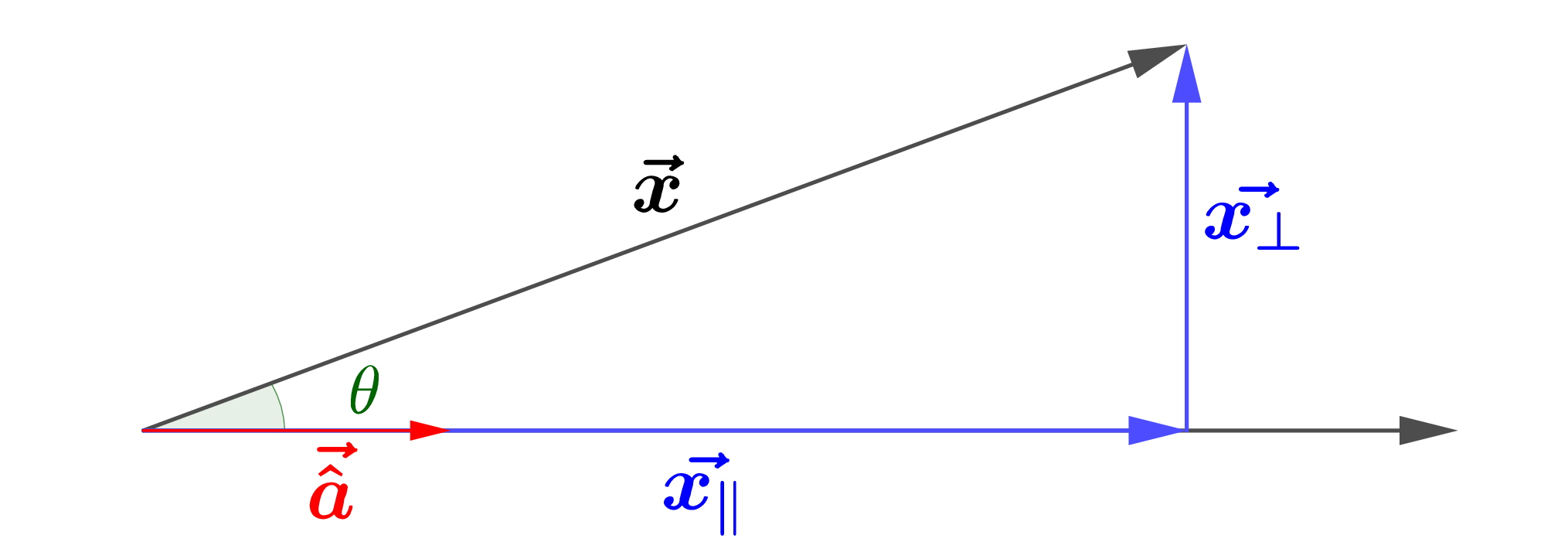
Figure 15: The vector 𝐱\mathbf{x} is decomposed into parallel and perpendicular commponents with respect to the vector 𝐚^\hat{\mathbf{a}}.

Given a vector 𝐱\mathbf{x} and a unit vector 𝐚^\hat{\mathbf{a}}, we wish to express 𝐱=𝐱∥+𝐱⟂\mathbf{x}=\mathbf{x}_{\parallel}+\mathbf{x}_{\perp} where 𝐱∥\mathbf{x}_{\parallel} is parallel to 𝐚^\hat{\mathbf{a}}, and 𝐱⟂\mathbf{x}_{\perp} is perpendicular to 𝐚^\hat{\mathbf{a}}, as shown in Figure 15. Since 𝐚^​𝐚^=1\hat{\mathbf{a}}\hat{\mathbf{a}}=1, and using the associative law,

𝐱=(𝐱​𝐚^)​𝐚^=(𝐱⋅𝐚^)​𝐚^+(𝐱∧𝐚^)​𝐚^=𝐱∥+𝐱⟂,\mathbf{x}=(\mathbf{x}\hat{\mathbf{a}})\hat{\mathbf{a}}=(\mathbf{x}\cdot\hat{\mathbf{a}})\hat{\mathbf{a}}+(\mathbf{x}\wedge\hat{\mathbf{a}})\hat{\mathbf{a}}=\mathbf{x}_{\parallel}+\mathbf{x}_{\perp},

where

𝐱∥=(𝐱⋅𝐚^)​𝐚^and𝐱⟂=(𝐱∧𝐚^)​𝐚^=𝐱−𝐱∥.\mathbf{x}_{\parallel}=(\mathbf{x}\cdot\hat{\mathbf{a}})\hat{\mathbf{a}}\quad{\rm and}\quad\mathbf{x}_{\perp}=(\mathbf{x}\wedge\hat{\mathbf{a}})\hat{\mathbf{a}}=\mathbf{x}-\mathbf{x}_{\parallel}.

We could also accomplish this decomposition by writing

𝐱=𝐚^​(𝐚^​𝐱)=𝐚^​(𝐚^⋅𝐱)+𝐚^​(𝐚^∧𝐱)=𝐱∥+𝐱⟂.\mathbf{x}=\hat{\mathbf{a}}(\hat{\mathbf{a}}\mathbf{x})=\hat{\mathbf{a}}(\hat{\mathbf{a}}\cdot\mathbf{x})+\hat{\mathbf{a}}(\hat{\mathbf{a}}\wedge\mathbf{x})=\mathbf{x}_{\parallel}+\mathbf{x}_{\perp}.

It follows that 𝐱∥=(𝐱⋅𝐚^)​𝐚^=𝐚^​(𝐱⋅𝐚^)\mathbf{x}_{\parallel}=(\mathbf{x}\cdot\hat{\mathbf{a}})\hat{\mathbf{a}}=\hat{\mathbf{a}}(\mathbf{x}\cdot\hat{\mathbf{a}}) as expected, and

𝐱⟂=(𝐱∧𝐚^)⋅𝐚^=𝐚^⋅(𝐚^∧𝐱)=−𝐚^⋅(𝐱∧𝐚^),\mathbf{x}_{\perp}=(\mathbf{x}\wedge\hat{\mathbf{a}})\cdot\hat{\mathbf{a}}=\hat{\mathbf{a}}\cdot(\hat{\mathbf{a}}\wedge\mathbf{x})=-\hat{\mathbf{a}}\cdot(\mathbf{x}\wedge\hat{\mathbf{a}}),

in agreement with (16).

Refer to caption
Figure 16: The line L𝐱0​(𝐚)L_{\mathbf{x}_{0}}(\mathbf{a}) through the point 𝐱0\mathbf{x}_{0} in the direction 𝐚\mathbf{a}.

One of the simplest problems in analytic geometry is given a vector 𝐚\mathbf{a} and a point 𝐱0\mathbf{x}_{0}, what is the equation of the line passing through the point 𝐱0\mathbf{x}_{0} in the direction of the vector 𝐚\mathbf{a}? The line L𝐱0​(𝐚)L_{\mathbf{x}_{0}}(\mathbf{a}) is given by

L𝐱0(𝐚):={𝐱|(𝐱−𝐱0)∧𝐚=0}.L_{\mathbf{x}_{0}}(\mathbf{a}):=\{\mathbf{x}|\ \ (\mathbf{x}-\mathbf{x}_{0})\wedge\mathbf{a}=0\}.

The equation

(𝐱−𝐱0)∧𝐚=0⇔𝐱=𝐱0+t𝐚,(\mathbf{x}-\mathbf{x}_{0})\wedge\mathbf{a}=0\ \ \iff\ \ \mathbf{x}=\mathbf{x}_{0}+t\mathbf{a},

for t∈ℝt\in\mathbb{R}, see Figure 16.

Refer to caption
Figure 17: The distance of the point 𝐩\mathbf{p} from the line L𝐱0​(𝐚)L_{\mathbf{x}_{0}}(\mathbf{a}) is |𝐱−𝐩||\mathbf{x}-\mathbf{p}|.

Given the line L𝐱0​(𝐚)L_{\mathbf{x}_{0}}(\mathbf{a}), and a point 𝐩\mathbf{p}, let us find the point 𝐱\mathbf{x} on the line L𝐱0​(𝐚)L_{\mathbf{x}_{0}}(\mathbf{a}) which is closest to the point 𝐩\mathbf{p}, and the distance |𝐱−𝐩||\mathbf{x}-\mathbf{p}| from 𝐱\mathbf{x} to 𝐩\mathbf{p}. Referring to Figure 17, and using the decomposition (4) to project 𝐩−𝐱0\mathbf{p}-\mathbf{x}_{0} onto the vector 𝐚^\hat{\mathbf{a}}, we find

𝐱=𝐱0+[(𝐩−𝐱0)⋅𝐚^]​𝐚^,\mathbf{x}=\mathbf{x}_{0}+[(\mathbf{p}-\mathbf{x}_{0})\cdot\hat{\mathbf{a}}]\hat{\mathbf{a}},

so, with the help of (9) and (4),

𝐱−𝐩=(𝐱0−𝐩)−[(𝐱0−𝐩)⋅𝐚^]​𝐚^=(𝐱0−𝐩)⟂,\mathbf{x}-\mathbf{p}=(\mathbf{x}_{0}-\mathbf{p})-[(\mathbf{x}_{0}-\mathbf{p})\cdot\hat{\mathbf{a}}]\hat{\mathbf{a}}=(\mathbf{x}_{0}-\mathbf{p})_{\perp}, (26)

where (𝐱0−𝐩)⟂(\mathbf{x}_{0}-\mathbf{p})_{\perp} is the component of 𝐱0−𝐩\mathbf{x}_{0}-\mathbf{p} perpendicular to 𝐚\mathbf{a}. Using (26), the distance of the point 𝐩\mathbf{p} to the line is

|𝐱−𝐩|=(𝐱−𝐩)2=(𝐱0−𝐩)2−((𝐱0−𝐩)⋅𝐚^)2=|(𝐱0−𝐩)⟂|,|\mathbf{x}-\mathbf{p}|=\sqrt{(\mathbf{x}-\mathbf{p})^{2}}=\sqrt{(\mathbf{x}_{0}-\mathbf{p})^{2}-\big((\mathbf{x}_{0}-\mathbf{p})\cdot\hat{\mathbf{a}}\big)^{2}}=|(\mathbf{x}_{0}-\mathbf{p})_{\perp}|,

see Figure 17.

4.1 The exponential function and rotations

The Euler exponential function arises naturally from the geometric product (9). With the help of (7) and (24), and noting that (I​𝐧^)2=−1(I\hat{\mathbf{n}})^{2}=-1, the geometric product of two unit vectors 𝐚^\hat{\mathbf{a}} and 𝐛^\hat{\mathbf{b}} in ℝ3\mathbb{R}^{3} is

𝐚^​𝐛^=𝐚^⋅𝐛^+𝐚^∧𝐛^=cos⁡θ+I​𝐧^​sin⁡θ=eθ​I​𝐧^,\hat{\mathbf{a}}\hat{\mathbf{b}}=\hat{\mathbf{a}}\cdot\hat{\mathbf{b}}+\hat{\mathbf{a}}\wedge\hat{\mathbf{b}}=\cos\theta+I\hat{\mathbf{n}}\sin\theta=e^{\theta I\hat{\mathbf{n}}}, (27)

where cos⁡θ:=𝐚^⋅𝐛^\cos\theta:=\hat{\mathbf{a}}\cdot\hat{\mathbf{b}}. Similarly,

𝐛^​𝐚^=𝐛^⋅𝐚^+𝐛^∧𝐚^=cos⁡θ−I​𝐧^​sin⁡θ=e−θ​I​𝐧^.\hat{\mathbf{b}}\hat{\mathbf{a}}=\hat{\mathbf{b}}\cdot\hat{\mathbf{a}}+\hat{\mathbf{b}}\wedge\hat{\mathbf{a}}=\cos\theta-I\hat{\mathbf{n}}\sin\theta=e^{-\theta I\hat{\mathbf{n}}}. (28)
Refer to caption
Figure 18: On the unit sphere, the arc 𝐚^​𝐛^~\widetilde{\hat{\mathbf{a}}\hat{\mathbf{b}}}, followed by the arc 𝐛^​𝐜^~\widetilde{\hat{\mathbf{b}}\hat{\mathbf{c}}}, gives the arc 𝐚^​𝐜^~\widetilde{\hat{\mathbf{a}}\hat{\mathbf{c}}}.

Let 𝐚^,𝐛^,𝐜^\hat{\mathbf{a}},\hat{\mathbf{b}},\hat{\mathbf{c}} be unit vectors in ℝ3\mathbb{R}^{3}. The equation

(𝐛^​𝐚^)​𝐚^=𝐛^​(𝐚^​𝐚^)=𝐛^=(𝐚​𝐚^)​𝐛^=𝐚^​(𝐚^​𝐛^),(\hat{\mathbf{b}}\hat{\mathbf{a}})\hat{\mathbf{a}}=\hat{\mathbf{b}}(\hat{\mathbf{a}}\hat{\mathbf{a}})=\hat{\mathbf{b}}=(\mathbf{a}\hat{\mathbf{a}})\hat{\mathbf{b}}=\hat{\mathbf{a}}(\hat{\mathbf{a}}\hat{\mathbf{b}}), (29)

shows that when 𝐚^\hat{\mathbf{a}} is multiplied on the right by 𝐚^​𝐛^=eθ​I​𝐧^\hat{\mathbf{a}}\hat{\mathbf{b}}=e^{\theta I\hat{\mathbf{n}}}, or on the left by 𝐛^​𝐚^=e−θ​I​𝐧^\hat{\mathbf{b}}\hat{\mathbf{a}}=e^{-\theta I\hat{\mathbf{n}}}, it rotates the vector 𝐚^\hat{\mathbf{a}} through the angle θ\theta into the vector 𝐛^\hat{\mathbf{b}}. The composition of rotations, can be pictured as the composition of arcs on the unit sphere. The composition of the arc 𝕒^​𝕓^~\widetilde{\mathbb{\hat{a}}\mathbb{\hat{b}}} on the great circle connecting the points 𝐚^\hat{\mathbf{a}} and 𝐛^\hat{\mathbf{b}}, with the arc 𝐛^​𝐜^~\widetilde{\hat{\mathbf{b}}\hat{\mathbf{c}}} connecting 𝐛^\hat{\mathbf{b}} and 𝐜^\hat{\mathbf{c}}, gives the arc 𝐚^​𝐜^~\widetilde{\hat{\mathbf{a}}\hat{\mathbf{c}}} connecting 𝐚^\hat{\mathbf{a}} and 𝐜^\hat{\mathbf{c}}. Symbolically,

𝐚^​𝐛^~​𝐛^​𝐜^~:=(𝐚^​𝐛^)​(𝐛^​𝐜^)=𝐚^​𝐜^=:𝐚^​𝐜^~,\widetilde{\hat{\mathbf{a}}\hat{\mathbf{b}}}\widetilde{\hat{\mathbf{b}}\hat{\mathbf{c}}}:=(\hat{\mathbf{a}}\hat{\mathbf{b}})(\hat{\mathbf{b}}\hat{\mathbf{c}})=\hat{\mathbf{a}}\hat{\mathbf{c}}=:\widetilde{\hat{\mathbf{a}}\hat{\mathbf{c}}},

as shown in

Refer to caption
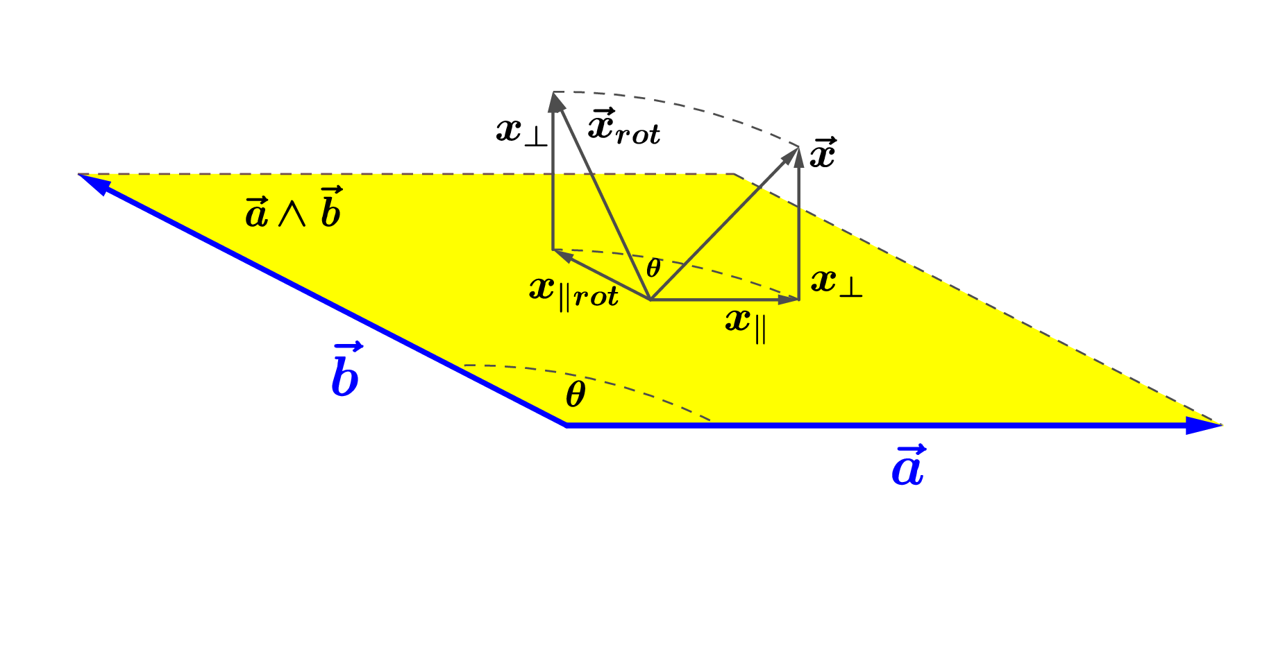
Figure 19: The parallel component 𝐱∥\mathbf{x}_{\parallel} of 𝐱\mathbf{x} in the plane of 𝐚∧𝐛\mathbf{a}\wedge\mathbf{b} is rotated through the angle θ\theta, leaving the perpendicular component 𝐱⟂\mathbf{x}_{\perp} unchanged.

Figure 18.

By taking the square roots of both sides of equations (27) and (28), it follows that

𝐚^​𝐛^=e12​θ​I​𝐧^,and𝐛^​𝐚^=e−12​θ​I​𝐧^.\sqrt{\hat{\mathbf{a}}\hat{\mathbf{b}}}=e^{\frac{1}{2}\theta I\hat{\mathbf{n}}},\quad{\rm and}\quad\sqrt{\hat{\mathbf{b}}\hat{\mathbf{a}}}=e^{-\frac{1}{2}\theta I\hat{\mathbf{n}}}.

Note also that

𝐛^=(𝐛^​𝐚^)​𝐚^=(𝐛^​𝐚^)2​𝐚^=𝐛^​𝐚^​𝐚^​𝐚^​𝐛^=e−12​θ​I​𝐧^​𝐚^​e12​θ​I​𝐧^.\hat{\mathbf{b}}=(\hat{\mathbf{b}}\hat{\mathbf{a}})\hat{\mathbf{a}}=(\sqrt{\hat{\mathbf{b}}\hat{\mathbf{a}}})^{2}\hat{\mathbf{a}}=\sqrt{\hat{\mathbf{b}}\hat{\mathbf{a}}}\ \hat{\mathbf{a}}\,\sqrt{\hat{\mathbf{a}}\hat{\mathbf{b}}}=e^{-\frac{1}{2}\theta I\hat{\mathbf{n}}}\hat{\mathbf{a}}\,e^{\frac{1}{2}\theta I\hat{\mathbf{n}}}. (30)

The advantage of the equation (30) over (29) is that it can be applied to rotate any vector 𝐱\mathbf{x}. For 𝐱=𝐱∥+𝐱⟂\mathbf{x}=\mathbf{x}_{\parallel}+\mathbf{x}_{\perp}, where 𝐱∥\mathbf{x}_{\parallel} is in the plane of 𝐚∧𝐛\mathbf{a}\wedge\mathbf{b}, and 𝐱⟂\mathbf{x}_{\perp} is perpendicular to the plane, we get with the help of (14) and (15),

𝐱r​o​t:=𝐛^​𝐚^​𝐱​𝐚^​𝐛^=e−12​θ​I​𝐧^​(𝐱∥+𝐱⟂)​e12​θ​I​𝐧^=e−θ​I​𝐧^​𝐱∥+𝐱⟂,\mathbf{x}_{rot}:=\sqrt{\hat{\mathbf{b}}\hat{\mathbf{a}}}\,\mathbf{x}\,\sqrt{\hat{\mathbf{a}}\hat{\mathbf{b}}}=e^{-\frac{1}{2}\theta I\hat{\mathbf{n}}}\,(\mathbf{x}_{\parallel}+\mathbf{x}_{\perp})e^{\frac{1}{2}\theta I\hat{\mathbf{n}}}=e^{-\theta I\hat{\mathbf{n}}}\mathbf{x}_{\parallel}+\mathbf{x}_{\perp}, (31)

see Figure 19. Formula (31) is known as the half angle representation of a rotation [11, p.55]. A rotation can also be expressed as the composition of two reflections.

4.2 Reflections

A bivector characterizes the direction of a plane. The equation of a plane passing through the origin in the direction of the bivector 𝐚∧𝐛\mathbf{a}\wedge\mathbf{b} is

Plane0(𝐚∧𝐛)={𝐱|𝐱∧𝐚∧𝐛=0}.Plane_{0}(\mathbf{a}\wedge\mathbf{b})=\{\mathbf{x}|\ \ \mathbf{x}\wedge\mathbf{a}\wedge\mathbf{b}=0\}. (32)

The condition that 𝐱∧𝐚∧𝐛=0\mathbf{x}\wedge\mathbf{a}\wedge\mathbf{b}=0 tells us that 𝐱\mathbf{x} is in the the plane of the bivector 𝐚∧𝐛\mathbf{a}\wedge\mathbf{b}, or

𝐱=ta​𝐚+tb​𝐛,\mathbf{x}=t_{a}\mathbf{a}+t_{b}\mathbf{b},

where ta,tb∈ℝt_{a},t_{b}\in\mathbb{R}. This is the parametric equation of a plane passing through the origin having the direction of the bivector 𝐚∧𝐛\mathbf{a}\wedge\mathbf{b}. If, instead, we want the equation of a plane passing through a given point 𝐱0\mathbf{x}_{0} and having the direction of the bivector 𝐚∧𝐛\mathbf{a}\wedge\mathbf{b}, we have

Plane𝐱0(𝐚∧𝐛)={𝐱|(𝐱−𝐱0)∧𝐚∧𝐛=0},Plane_{\mathbf{x}_{0}}(\mathbf{a}\wedge\mathbf{b})=\{\mathbf{x}|\ \ (\mathbf{x}-\mathbf{x}_{0})\wedge\mathbf{a}\wedge\mathbf{b}=0\}, (33)

with the corresponding parametric equation

𝐱=𝐱0+ta​𝐚+tb​𝐛.\mathbf{x}=\mathbf{x}_{0}+t_{a}\mathbf{a}+t_{b}\mathbf{b}.

For a plane in ℝ3\mathbb{R}^{3}, when 𝐱=(x,y,z)\mathbf{x}=(x,y,z) and 𝐱0=(x0,y0,z0)\mathbf{x}_{0}=(x_{0},y_{0},z_{0}), using (25) and (33),

Plane𝐱0(𝐚∧𝐛)={𝐱|det(x−x0y−y0z−z0a1a2a3b1b2b3)=0},Plane_{\mathbf{x}_{0}}(\mathbf{a}\wedge\mathbf{b})=\{\mathbf{x}|\ \ \det{\pmatrix{x-x_{0}&y-y_{0}&z-z_{0}\cr a_{1}&a_{2}&a_{3}\cr b_{1}&b_{2}&b_{3}}}=0\},

which is equivalent to the well known equation of a line through the point 𝐱0\mathbf{x}_{0},

(𝐱−𝐱0)⋅𝐧=0,(\mathbf{x}-\mathbf{x}_{0})\cdot\mathbf{n}=0,

where 𝐧=𝐚×𝐛\mathbf{n}=\mathbf{a}\times\mathbf{b} is the normal vector to the bivector 𝐚∧𝐛\mathbf{a}\wedge\mathbf{b} of the plane, see Figure 20.

Refer to caption
Figure 20: The point 𝐱\mathbf{x} is in the plane passing through the point x0x_{0} and having the direction of the bivector 𝐚∧𝐛\mathbf{a}\wedge\mathbf{b}.

Given a vector 𝐱\mathbf{x} and a unit bivector 𝐚∧𝐛\mathbf{a}\wedge\mathbf{b}, we decompose 𝐱\mathbf{x} into a part 𝐱∥\mathbf{x}_{\parallel} parallel to 𝐚∧𝐛\mathbf{a}\wedge\mathbf{b}, and a part 𝐱⟂\mathbf{x}_{\perp} perpendicular to 𝐚∧𝐛\mathbf{a}\wedge\mathbf{b}. Since by (15)

𝐱∥∧𝐚∧𝐛=12​(𝐱∥​(𝐚∧𝐛)+(𝐚∧𝐛)​𝐱∥)=0,\mathbf{x}_{\parallel}\wedge\mathbf{a}\wedge\mathbf{b}=\frac{1}{2}\Big(\mathbf{x}_{\parallel}(\mathbf{a}\wedge\mathbf{b})+(\mathbf{a}\wedge\mathbf{b})\mathbf{x}_{\parallel}\Big)=0,

and by (14),

𝐱⟂⋅(𝐚∧𝐛)=12​(𝐱⟂​(𝐚∧𝐛)−(𝐚∧𝐛)​𝐱⟂)=0,\mathbf{x}_{\perp}\cdot(\mathbf{a}\wedge\mathbf{b})=\frac{1}{2}\Big(\mathbf{x}_{\perp}(\mathbf{a}\wedge\mathbf{b})-(\mathbf{a}\wedge\mathbf{b})\mathbf{x}_{\perp}\Big)=0,

it follows that the parallel and perpendicular parts of 𝐱\mathbf{x} anti-commute and commute, respectively, with the bivector 𝐚∧𝐛\mathbf{a}\wedge\mathbf{b}. Remembering that (𝐚∧𝐛)2=−1(\mathbf{a}\wedge\mathbf{b})^{2}=-1, it follows that

(𝐚∧𝐛)​𝐱​(𝐚∧𝐛)=(𝐚∧𝐛)​(𝐱∥+𝐱⟂)​(𝐚∧𝐛)=𝐱∥−𝐱⟂.(\mathbf{a}\wedge\mathbf{b})\mathbf{x}(\mathbf{a}\wedge\mathbf{b})=(\mathbf{a}\wedge\mathbf{b})(\mathbf{x}_{\parallel}+\mathbf{x}_{\perp})(\mathbf{a}\wedge\mathbf{b})=\mathbf{x}_{\parallel}-\mathbf{x}_{\perp}. (34)

This is the general formula for the reflection of a vector 𝐱\mathbf{x} in a mirror in the plane of the unit bivector 𝐚∧𝐛\mathbf{a}\wedge\mathbf{b}.

When we are in the 33-dimensional space ℝ3\mathbb{R}^{3}, the unit bivector

𝐚∧𝐛=I⁡(𝐚×𝐛)=I​𝐧^.\mathbf{a}\wedge\mathbf{b}=I(\mathbf{a}\times\mathbf{b})=I\hat{\mathbf{n}}.

In this case, the reflection (34) takes the form

(𝐚∧𝐛)​𝐱​(𝐚∧𝐛)=−𝐧^​𝐱​𝐧^=−𝐧^​(𝐱∥+𝐱⟂)​𝐧^=𝐱∥−𝐱⟂.(\mathbf{a}\wedge\mathbf{b})\mathbf{x}(\mathbf{a}\wedge\mathbf{b})=-\hat{\mathbf{n}}\mathbf{x}\hat{\mathbf{n}}=-\hat{\mathbf{n}}(\mathbf{x}_{\parallel}+\mathbf{x}_{\perp})\hat{\mathbf{n}}=\mathbf{x}_{\parallel}-\mathbf{x}_{\perp}. (35)

Since a rotation in ℝ3\mathbb{R}^{3} is generated by two consecutive reflections about two planes with normal unit vectors 𝐧^1\hat{\mathbf{n}}_{1} and 𝐧^2\hat{\mathbf{n}}_{2}, we have

𝐱r​o​t=−𝐧^2​(−𝐧^1​𝐱​𝐧^1)​𝐧^2=(𝐧^2​𝐧^1)​𝐱​(𝐧^1​𝐧^2).\mathbf{x}_{rot}=-\hat{\mathbf{n}}_{2}(-\hat{\mathbf{n}}_{1}\mathbf{x}\hat{\mathbf{n}}_{1})\hat{\mathbf{n}}_{2}=(\hat{\mathbf{n}}_{2}\hat{\mathbf{n}}_{1})\mathbf{x}(\hat{\mathbf{n}}_{1}\hat{\mathbf{n}}_{2}). (36)

Letting 𝐧^1​𝐧^2=e12​θ​I​𝐧^\hat{\mathbf{n}}_{1}\hat{\mathbf{n}}_{2}=e^{\frac{1}{2}\theta I\hat{\mathbf{n}}} where

𝐧^:=𝐧^1×𝐧^2|𝐧^1×𝐧^2|,\hat{\mathbf{n}}:=\frac{\hat{\mathbf{n}}_{1}\times\hat{\mathbf{n}}_{2}}{|\hat{\mathbf{n}}_{1}\times\hat{\mathbf{n}}_{2}|},

the formula for the rotation (36) becomes

𝐱r​o​t=(𝐧^2​𝐧^1)​𝐱​(𝐧^1​𝐧^2)=e−12​θ​I​𝐧^​𝐱​e12​θ​I​𝐧^=e−12​θ​I​𝐧^​𝐱∥​e12​θ​I​𝐧^+𝐱⟂,\mathbf{x}_{rot}=(\hat{\mathbf{n}}_{2}\hat{\mathbf{n}}_{1})\mathbf{x}(\hat{\mathbf{n}}_{1}\hat{\mathbf{n}}_{2})=e^{-\frac{1}{2}\theta I\hat{\mathbf{n}}}\mathbf{x}e^{\frac{1}{2}\theta I\hat{\mathbf{n}}}=e^{-\frac{1}{2}\theta I\hat{\mathbf{n}}}\mathbf{x}_{\parallel}e^{\frac{1}{2}\theta I\hat{\mathbf{n}}}+\mathbf{x}_{\perp}, (37)

which is equivalent to (31).

5 Stereographic projection and a bit of quantum mechanics

Refer to caption
Figure 21: Stereographic Projection from the South Pole of S2S^{2} to the x​yxy-plane, where 𝐦=𝐱+𝐞3\mathbf{m}=\mathbf{x}+\mathbf{e}_{3} and 𝐦^=𝐦|𝐦|\hat{\mathbf{m}}=\frac{\mathbf{m}}{|\mathbf{m}|}.

As a final demonstration of the flexibility and power of geometric algebra, we discuss stereographic projection from the unit sphere S2⊂ℝ3S^{2}\subset\mathbb{R}^{3}, defined by

S2:={𝐚^|𝐚^2=1and𝐚^∈ℝ3},S^{2}:=\{\hat{\mathbf{a}}|\quad\hat{\mathbf{a}}^{2}=1\ \ {\rm and}\ \ \hat{\mathbf{a}}\in\mathbb{R}^{3}\},

onto ℝ2\mathbb{R}^{2}. The mapping 𝐱=f⁡(𝐚^)∈ℝ2\mathbf{x}=f(\hat{\mathbf{a}})\in\mathbb{R}^{2} defining stereographic projection is

𝐱=f⁡(𝐚^):=2𝐚^+𝐞3−𝐞3,where𝐚^∈S2,\mathbf{x}=f(\hat{\mathbf{a}}):=\frac{2}{\hat{\mathbf{a}}+\mathbf{e}_{3}}-\mathbf{e}_{3},\ \ {\rm where}\ \ \hat{\mathbf{a}}\in S^{2}, (38)

and is pictured in Figure 21. A 2-D cut away in the plane of the great circle, defined by the points 𝐞3,𝐚^\mathbf{e}_{3},\hat{\mathbf{a}}, and the origin, is shown in Figure 22. Stereographic projection is an example of a conformal mapping, which preserves angles, and has many important applications in mathematics, physics, and more recently in robotics [2, 10].

[Uncaptioned image]
Figure 22: A 2-D cut away in the plane of great circle through the points 𝐞3,𝐚^\mathbf{e}_{3},\hat{\mathbf{a}}, and −𝐚^-\hat{\mathbf{a}} on S2S^{2}.

In working with the mapping (38), it is convenient to use the new variable 𝐦=𝐱+𝐞3\mathbf{m}=\mathbf{x}+\mathbf{e}_{3}, for which case the mapping takes the simpler form

𝐦=2𝐚^+𝐞3=2​(𝐚^+𝐞3)(𝐚^+𝐞3)2=𝐚^+𝐞31+𝐚^⋅𝐞3.\mathbf{m}=\frac{2}{\hat{\mathbf{a}}+\mathbf{e}_{3}}=\frac{2(\hat{\mathbf{a}}+\mathbf{e}_{3})}{(\hat{\mathbf{a}}+\mathbf{e}_{3})^{2}}=\frac{\hat{\mathbf{a}}+\mathbf{e}_{3}}{1+\hat{\mathbf{a}}\cdot\mathbf{e}_{3}}. (39)

The effect of this change of variable maps points 𝐱∈ℝ3\mathbf{x}\in\mathbb{R}^{3} into corresponding points 𝐦\mathbf{m} in the plane P​l​a​n​e𝐞3​(𝐞12)Plane_{\mathbf{e}_{3}}(\mathbf{e}_{12}) passing through the point 𝐞3\mathbf{e}_{3} and parallel to ℝ2=P​l​a​n​e0​(𝐞12)\mathbb{R}^{2}=Plane_{0}(\mathbf{e}_{12}). Noting that

𝐞3⋅𝐦=𝐞3⋅(𝐚^+𝐞31+𝐚^⋅𝐞3)=1,\mathbf{e}_{3}\cdot\mathbf{m}=\mathbf{e}_{3}\cdot\Big(\frac{\hat{\mathbf{a}}+\mathbf{e}_{3}}{1+\hat{\mathbf{a}}\cdot\mathbf{e}_{3}}\Big)=1,

and solving the equation (39) for 𝐚^\hat{\mathbf{a}}, gives with the help of (3) and (8),

𝐚^=2𝐦−𝐞3=𝐦−1​(2−𝐦𝐞3)\hat{\mathbf{a}}=\frac{2}{\mathbf{m}}-\mathbf{e}_{3}=\mathbf{m}^{-1}\big(2-\mathbf{m}\mathbf{e}_{3}\big)
=𝐦^|𝐦|​(2+𝐞3​𝐦−2​𝐞3⋅𝐦)=𝐦^​𝐞3​𝐦^.=\frac{\hat{\mathbf{m}}}{|\mathbf{m}|}\big(2+\mathbf{e}_{3}\mathbf{m}-2\mathbf{e}_{3}\cdot\mathbf{m}\big)=\hat{\mathbf{m}}\mathbf{e}_{3}\hat{\mathbf{m}}. (40)

We also have

𝐚^=𝐦^​𝐞3​𝐦^=(𝐦^​𝐞3)​𝐞3​(𝐞3​𝐦^)=(−I​𝐦^)​𝐞3​(I​𝐦^),\hat{\mathbf{a}}=\hat{\mathbf{m}}\mathbf{e}_{3}\hat{\mathbf{m}}=(\hat{\mathbf{m}}\mathbf{e}_{3})\mathbf{e}_{3}(\mathbf{e}_{3}\hat{\mathbf{m}})=(-I\hat{\mathbf{m}})\mathbf{e}_{3}(I\hat{\mathbf{m}}), (41)

showing that 𝐚^\hat{\mathbf{a}} is obtained by a rotation of 𝐞3\mathbf{e}_{3} in the plane of 𝐦^∧𝐞3\hat{\mathbf{m}}\wedge\mathbf{e}_{3} through an angle of 2​θ2\theta where cos⁡θ:=𝐞3⋅𝐦^\cos\theta:=\mathbf{e}_{3}\cdot\hat{\mathbf{m}}, or equivalently, by a rotation of 𝐞3\mathbf{e}_{3} in the plane of I​𝐦^I\hat{\mathbf{m}} through an angle of π\pi.

Quantum mechanics displays many surprising, amazing, and almost magical properties, which defy the classical mechanics of everyday experience. If the quantum spin state of an electron is put into a spin state 𝐚^∈S2\hat{\mathbf{a}}\in S^{2} by a strong magnetic field at a given time, then the probability of observing the electron’s spin in the spin state 𝐛^∈S2\hat{\mathbf{b}}\in S^{2} at a time immediately thereafter is

p​r​o​b𝐚^+​(𝐛^):=12​(1+𝐚^⋅𝐛^)=1−(𝐦a−𝐦b)2𝐦a2​𝐦b2,prob_{\hat{\mathbf{a}}}^{+}(\hat{\mathbf{b}}):=\frac{1}{2}(1+\hat{\mathbf{a}}\cdot\hat{\mathbf{b}})=1-\frac{(\mathbf{m}_{a}-\mathbf{m}_{b})^{2}}{\mathbf{m}_{a}^{2}\mathbf{m}_{b}^{2}}, (42)

where

𝐚^=2𝐦a−𝐞3and𝐛^=2𝐦b−𝐞3,\hat{\mathbf{a}}=\frac{2}{\mathbf{m}_{a}}-\mathbf{e}_{3}\quad{\rm and}\quad\hat{\mathbf{b}}=\frac{2}{\mathbf{m}_{b}}-\mathbf{e}_{3},

see [13, 16].

On the other hand, the probability of a photon being emitted by an electron prepared in a spin state 𝐛^\hat{\mathbf{b}}, when it is forced by a magnetic field into the spin state 𝐚^\hat{\mathbf{a}} is

p​r​o​b𝐚^−​(𝐛^):=12​(1−𝐚^⋅𝐛^)=(𝐦a−𝐦b)2𝐦a2​𝐦b2.prob_{\hat{\mathbf{a}}}^{-}(\hat{\mathbf{b}}):=\frac{1}{2}(1-\hat{\mathbf{a}}\cdot\hat{\mathbf{b}})=\frac{(\mathbf{m}_{a}-\mathbf{m}_{b})^{2}}{\mathbf{m}_{a}^{2}\mathbf{m}_{b}^{2}}. (43)

Whenever a photon is emitted, it has exactly the same energy, regardless of the angle θ\theta between the spin states 𝐚^\hat{\mathbf{a}} and 𝐛^\hat{\mathbf{b}}, [17, 18]. A plot of these two probability functions is given in Figure 23. The equalities in (42) and (43) show that p​r​o​b𝐚^±​(𝐛^)prob_{\hat{\mathbf{a}}}^{\pm}(\hat{\mathbf{b}}) is directly related to the Euclidean distances between the points 𝐦a,𝐦b∈P​l​a​n​e𝐞3​(𝐞12)\mathbf{m}_{a},\mathbf{m}_{b}\in Plane_{\mathbf{e}_{3}}(\mathbf{e}_{12}). The case when

𝐦a=𝐦=𝐱+𝐞3,𝐛^=−𝐚^,and𝐦b=𝐦⟂=−1𝐱+𝐞3\mathbf{m}_{a}=\mathbf{m}=\mathbf{x}+\mathbf{e}_{3},\ \ \hat{\mathbf{b}}=-\hat{\mathbf{a}},\ \ {\rm and}\ \ \mathbf{m}_{b}=\mathbf{m}_{\perp}=-\frac{1}{\mathbf{x}}+\mathbf{e}_{3}

is pictured in Figure 22.

[Uncaptioned image]
Figure 23: The functions p​r​o​b𝐚^±​(𝐛^)prob_{\hat{\mathbf{a}}}^{\pm}(\hat{\mathbf{b}}). The angle 0≤θ≤π0\leq\theta\leq\pi is between the unit vectors 𝐚^\hat{\mathbf{a}} and 𝐛^\hat{\mathbf{b}}.

References

  • [1] W.K. Clifford, Applications of Grassmann’s extensive algebra, Am. J. Math (ed.), Mathematical Papers by William Kingdon Clifford, pp. 397-401, Macmillan, London (1882). (Reprinted by Chelsea, New York, 1968.)
  • [2] E.B. Corrochano, G. Sobczyk, Editors, Geometric Algebra with Applications in Science and Engineering, Birkhäuser (2001).
  • [3] M.J. Crowe, A History of Vector Analysis, Dover, New York (1985).
  • [4] T. Dantzig, Number: The Language of Science, 4th edn. Free Press, New York 1967.
  • [5] C. Doran, A. Lasenby, Geometric Algebra for Physicists, Cambridge 2007.
  • [6] T. F. Havel, J.L. Doran, Geometric Algebra in Quantum Information Processing, Contemporary Mathematics, ISBN-10: 0-8218-2140-7, Vol. 305, 2002.
  • [7] D. Hestenes and G. Sobczyk. Clifford Algebra to Geometric Calculus: A Unified Language for Mathematics and Physics, 2nd edition, Kluwer 1992.
  • [8] P. Lounesto, Clifford Algebras and Spinors, 2nd Edition. Cambridge University Press, Cambridge, 2001.
  • [9] G. Sobczyk, Hyperbolic Number Plane, The College Mathematics Journal, Vol. 26, No. 4, pp.268-280, September 1995.
  • [10] G. Sobczyk, Conformal Mappings in Geometric Algebra, Notices of the AMS, Volume 59, Number 2, p.264-273, 2012.
  • [11] G. Sobczyk, New Foundations in Mathematics: The Geometric Concept of Number, Birkhäuser, New York 2013.
  • [12] G. Sobczyk, Geometric Spinors, Relativity and the Hopf Fibration, http://www.garretstar.com/geo2hopf26-9-2015.pdf
  • [13] G. Sobczyk, Part I: The Vector Analysis of Spinors (2016) http://www.garretstar.com/paulispin-19-07-2015.pdf
    https://arxiv.org/pdf/1507.06608.pdf
  • [14] G. Sobczyk, Geometrization of the Real Number System, July 2017. http://www.garretstar.com/geonum2017.pdf
  • [15] G. Sobczyk, Hyperbolic Numbers Revisted, Dec. 2017. http://www.garretstar.com/hyprevisited12-17-2017.pdf
  • [16] G. Sobczyk, Spinors in Spacetime Algebra and Euclidean 4-Space (2017)
    https://arxiv.org/pdf/1703.01244.pdf
  • [17] L. Susskind, Lecture Notes 2: Electron Spin, Stanford University (2006).
    http://www.lecture-notes.co.uk/susskind/quantum-entanglements/lecture-2/electron-spin/
  • [18] L. Susskind, YouTube: Quantum Entanglements, Lecture 2
    https://www.youtube.com/playlist?list=PL8D12D5AADF422C5D&feature=plcp