Discriminative Label Consistent Domain Adaptation

To meet property P2, we follow JDA[21] and explicitly leverage MMD in RKHS to measure the distances between the expectations of the source domain/sub-domain and target domain/sub-domain: 1) The empirical distance of the source and target domains are defined as $Dis{t^{m}}$. 2) The conditional distance $Dis{t^{c}}$ is defined as the sum of the empirical distances between sub-domains in ${{\cal D}_{\cal S}}$ and ${{\cal D}_{\cal T}}$ with a same label $c$.

where $C$ is the number of classes, $\mathcal{D_{S}}^{(c)}=\{{x_{i}}:{x_{i}}\in\mathcal{D_{S}}\wedge y({x_{i}}=c)\}$ represents the ${c^{th}}$ sub-domain in the source domain. $\mathcal{D_{T}}^{(c)}$ is defined similarly for the target domain. ${{\bf{M}}_{0}}$ represents the marginal distribution between ${{\cal D}_{\cal S}}$ and ${{\cal D}_{\cal T}}$with ${{{({{\bf{M}}_{0}})}_{ij}}=\frac{1}{{{n_{s}}{n_{s}}}}}$ if $({{x_{i}},{x_{j}}\in{D_{S}}})$, ${{{({{\bf{M}}_{0}})}_{ij}}=\frac{1}{{{n_{t}}{n_{t}}}}}$ if $({{x_{i}},{x_{j}}\in{D_{T}}})$ and ${{{({{\bf{M}}_{0}})}_{ij}}=0}$ otherwise. $\bf M_{c}$ represents the conditional distribution between the sub-domains $c$ in ${{\cal D}_{\cal S}}$ and ${{\cal D}_{\cal T}}$ with ${{{({{\bf{M}}_{c}})}_{ij}}=\frac{1}{{n_{s}^{(c)}n_{s}^{(c)}}}}$ if $({{x_{i}},{x_{j}}\in{D_{S}}^{(c)}})$, ${{{({{\bf{M}}_{c}})}_{ij}}=\frac{1}{{n_{t}^{(c)}n_{t}^{(c)}}}}$ if $({{x_{i}},{x_{j}}\in{D_{T}}^{(c)}})$, ${{{({{\bf{M}}_{c}})}_{ij}}=\frac{{-1}}{{n_{s}^{(c)}n_{t}^{(c)}}}}$ if $({{x_{i}}\in{D_{S}}^{(c)},{x_{j}}\in{D_{T}}^{(c)}\;or\;\;{x_{i}}\in{D_{T}}^{(c)},{x_{j}}\in{D_{S}}^{(c)}})$ and ${{{({{\bf{M}}_{c}})}_{ij}}=0}$ otherwise. $n_{s}^{(c)}$ is the number of samples in the ${c^{th}}$ source sub-domain and $n_{t}^{(c)}$ is defined similarly for the ${c^{th}}$ target sub-domain .

The discrepancy between the marginal distributions $\mathcal{P}(\mathcal{X_{S}})$ and $\mathcal{P}(\mathcal{X_{T}})$ can be reduced in minimizing $Dis{t^{m}}$ whereas the mismatches of conditional distributions between ${{D_{\cal S}}^{c}}$ and ${{D_{\cal T}}^{c}}$ can be decreased in minimizing ${Dis{t^{c}}}$. In summary, the discrepancies of both the marginal and conditional distributions between the source and target can be jointly reduced in minimizing $Dis{t_{C}}$.

Aligning data distributions as does the previous sub-section does not guarantee that both the source and target data are discriminative with respect to the class labels. To satisfy property P1 and P3, we introduce a repulsive force term $Dist_{{\cal S}\to{\cal S}}^{re}$, where ${{\cal S}\to{\cal S}}$ indexes the distances computed from ${D_{\cal S}}$ to ${D_{\cal S}}$. $Dist_{{\cal S}\to{\cal S}}^{re}$ represents the sum of the distances from each source sub-domain ${D_{\cal S}}^{(c)}$ to all the other source sub-domains ${D_{\cal S}}^{(r);\;r\in\{\{1...C\}-\{c\}\}}$, excluding the $c$-th source sub-domain:

Eq.(4) is calculated in a similar way as Eq.(3), with ${{{({{\bf{M}}_{{\bf{S}}\to{\bf{S}}}})}_{ij}}=\frac{1}{{n_{s}^{(c)}n_{s}^{(c)}}}}$ if ${({x_{i}},{x_{j}}\in{D_{S}}^{(c)})}$, ${\frac{1}{{n_{s}^{(r)}n_{s}^{(r)}}}}$ if ${({x_{i}},{x_{j}}\in{D_{S}}^{(r)})}$, ${\frac{{-1}}{{n_{s}^{(c)}n_{s}^{(r)}}}}$ if ${({x_{i}}\in{D_{S}}^{(c)},{x_{j}}\in{D_{S}}^{(r)}\;or\;{x_{i}}\in{D_{S}}^{(r)},{x_{j}}\in{D_{S}}^{(c)})}$ and ${0}$ otherwise.

Similarly, we can also introduce a repulsive force term $Dist_{{\cal S}\to{\cal T}}^{re}+Dist_{{\cal T}\to{\cal S}}^{re}$ between the source sub-domains and those in the target domain, where ${{\cal S}\to{\cal T}}$ and ${{\cal T}\to{\cal S}}$ index the distances computed from ${D_{\cal S}}$ to ${D_{\cal T}}$ and those from ${D_{\cal T}}$ to ${D_{\cal S}}$, respectively. $Dist_{{\cal S}\to{\cal T}}^{re}$ represents the sum of the distances between each source sub-domain ${D_{\cal S}}^{(c)}$ and all the target sub-domains ${D_{\cal T}}^{(r);\;r\in\{\{1...C\}-\{c\}\}}$ excluding the $c$-th target sub-domain. $Dist_{{\cal T}\to{\cal S}}^{re}$ represents the sum of the distances from each target sub-domain ${D_{\cal T}}^{(c)}$ to all the the source sub-domains ${D_{\cal S}}^{(r);\;r\in\{\{1...C\}-\{c\}\}}$ excluding the $c$-th source sub-domain. These two distances are explicitly defined as:

Eq.(5) is defined in a similar way as Eq.(4) and Eq.(3), where ${{{({{\bf{M}}_{{\bf{S}}\to{\bf{T}}}})}_{ij}}=\frac{1}{{n_{s}^{(c)}n_{s}^{(c)}}}}$ if $({{x_{i}},{x_{j}}\in{D_{S}}^{(c)}})$, ${\frac{1}{{n_{t}^{(r)}n_{t}^{(r)}}}}$ if $({{x_{i}},{x_{j}}\in{D_{T}}^{(r)}})$, ${\frac{{-1}}{{n_{s}^{(c)}n_{t}^{(r)}}}}$ if $({{x_{i}}\in{D_{S}}^{(c)},{x_{j}}\in{D_{T}}^{(r)}\;or\;{x_{i}}\in{D_{T}}^{(r)},{x_{j}}\in{D_{S}}^{(c)}})$ and ${0}$ otherwise; ${{{({{\bf{M}}_{{\bf{T}}\to{\bf{S}}}})}_{ij}}=\frac{1}{{n_{t}^{(c)}n_{t}^{(c)}}}}$ if ${({x_{i}},{x_{j}}\in{D_{T}}^{(c)})}$, ${\frac{1}{{n_{s}^{(r)}n_{s}^{(r)}}}}$ if ${({x_{i}},{x_{j}}\in{D_{S}}^{(r)})}$, ${\frac{{-1}}{{n_{t}^{(c)}n_{s}^{(r)}}}}$ if ${({x_{i}}\in{D_{T}}^{(c)},{x_{j}}\in{D_{S}}^{(r)}\;or\;{x_{i}}\in{D_{S}}^{(r)},{x_{j}}\in{D_{T}}^{(c)})}$ and ${0}$ otherwise.

Finally, in integrating Eq.(4) and Eq.(5), we obtain the final repulsive force term as

We further define ${{\bf{M}}_{REP}}={{\bf{M}}_{S\to T}}+{{\bf{M}}_{T\to S}}+{{\bf{M}}_{S\to S}}$ as the repulsive force constraint matrix.

The maximization of Eq.(6) increases the distances between source sub-domains as well as those between source and target sub-domains, thereby enhancing the discriminative power of the underlying latent feature space.

Eq.(3) and Eq.(6) do not explicitly optimize the prediction errors of a learned hypothesis on the source data nor ensure label consistencies between the source and target domain.

To meet P1 and P4 and thereby explicitly optimize the first and the third term in Eq.(1), we introduce a novel label regression consistency constraint $\Phi({\bf{A}},{{\bf{Y}}_{S}},{{\bf{X}}_{S}})$, where A is the transformation matrix projecting both the source and target data into a latent shared feature subspace of dimension $k$. Specifically, we first embed each $C$-dimensional label vector into the $k$-dimensional latent shared feature subspace by adding $(C-k+1)$ times $0$. We can then perform class label regression and explicitly enhance class prediction accuracy on the source data and the class label consistency between the source and target domains through the least square regression (LSR): $\min\left\|{{{\bf{X}}^{T}}{\bf{A}}-{\bf{Y}}}\right\|_{F}^{2}$ ${\rm{s}}t.{\bf{Y}}\geq{\bf{0}},\;{\bf{Y1}}={\bf{1}}$, with Y the class label matrix as defined in Section 3.1 and extended into a $n\times k$ matrix by embedding each label vector into a $k$-dimensional unit vector. This constraint simply expresses that each data sample should be projected in the vicinity of its corresponding unit label vector in the latent shared feature subspace.

As source and target data can be noisy, we also introduce a matrix E to model noise. As a result, the LSR can be reformulated as: $\min\left\|{{{\bf{X}}^{T}}{\bf{A}}-{\bf{Y}}+{\bf{E}}}\right\|_{F}^{2}$ ${\rm{s}}t.\;{\bf{Y}}\geq{\bf{0}},\;{\bf{Y1}}={\bf{1}}$. The introduction of the error matrix E enables to account for outliers and thereby alleviate the influence of negative transfer to meet property P4.

In many real-life applications, especially in the field of visual recognition, data of a given class generally lie within a manifold of much lower dimension in comparison with the original data space, e.g., pixel number of images. Therefore, we further introduce a ${l_{2,1}}$-norm constraint so as to express the property that the class label of a data sample should be regressed from a sparse combination of features in the latent shared feature subspace. This constraint introduces a regularization term on A for discriminative subspace projection.

The label regression consistency constraint is finally formulated as

In integrating all the properties expressed in the previous subsections, i.e., Eq.(3), Eq.(6) and Eq.(7), we obtain our final DA model, formulated as Eq.(8)

Through iterative optimization of Eq.(8), our DA method searches jointly a latent subspace and a label regression model satisfying at the same time properties P1 through P5.

We follow the experimental settings of JDA, LTSL, DAN and LRSR, and apply DeCAF6 as the features for some methods to be evaluated. However, whenever possible in these figures, we directly report the performance scores from the publications, i.e., [21, 33, 6, 10, 36, 37, 11] , of the twenty-three methods listed above. They are assumed to be their best performance.

As can be seen from Fig.2 and Fig.3, the experimental results verify the effectiveness of the proposed DLC-DA method which consistently outperforms state-of-the-art DA methods, whether with the traditional shallow SURF features or the deep DeCAF6 features. However, given such a performance, one natural question that one can raise is how the proposed method is sensitive to the choice of the hyper-parameters. This issue is analyzed in the next subsection.

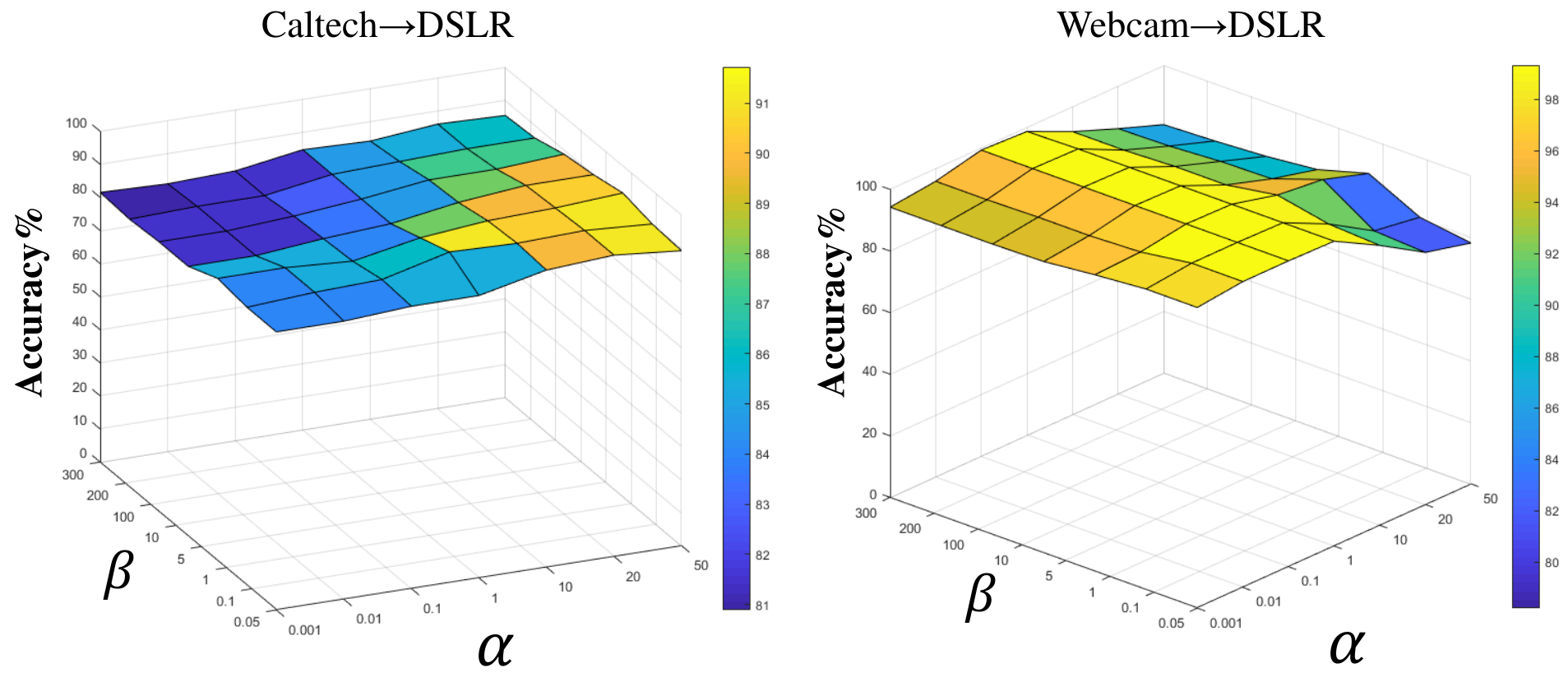
$\alpha$ and $\beta$ as defined in Eq.(8) are the major hyper-parameters of the proposed DLC-DA method. While $\alpha$ aims to regularize the projection matrix $A$ to avoid over-fitting the chosen shared feature subspace with respect to both source and target data, $\beta$ as expressed in Eq.(7) controls the dimensionality of class dependent data manifold in the searched shared feature subspace, or in other word the sparsity level of the linear combination of the projected features to regress the class label. We study the sensitivity of the proposed DLC-DA method with a wide range of parameter values, i.e., $\alpha=(0.001,0.01,0.1,1,10,20,50)$ and $\beta=(0.05,0.1,1,5,10,100,200)$. We only report the results on C $\rightarrow$ D $and$ W $\rightarrow$ D datasets due to the space limitation. With $k$ held fixed at $100$, Fig.4 illustrates these results. As can be seen from Fig.4, the proposed DLC-DA displays its stability as the resultant classification accuracies remain roughly the same despite a wide range of $\alpha$ and $\beta$ values.

In Fig.5, We further perform a convergence analysis of the proposed DLC-DA method, namely the performance convergence w.r.t. the number of iterations $T$, as well as the impact of the chosen dimensionality, i.e., $k$, of the searched shared feature subspace. We report the results on D $\rightarrow$ W, W $\rightarrow$ C $and$ D $\rightarrow$ A. In Fig.5.a, we vary the number of iterations $T=(1,2,3,4,5,6,7,8,9,10)$, whereas the subspace dimensionality $k$ varies with $k=(20,40,60,80,100,120,140,160,180,200)$ in Fig.5.b. As can be seen from Fig.5.a, the proposed DLC-DA achieves its optimal performance only after 2 iterations. Furthermore, Fig.5. shows that DLC-DA remains stable w.r.t. a wide rang of $k\in[20,200]$.

The core model of the proposed DLC-DA method is Eq.(8) which adds up two optimization terms, namely discriminative data distribution alignment (DDA) term as defined in Eq.(19), and label consistent regression (LCR) term as defined in Eq.(7). The DDA and LCR term aim to decrease discriminatively data distribution mismatch and ensure label consistency as defined by the second and third term of the error bound in Eq.(1). One interesting question is how each of these terms contributes to the proposed final model as defined by Eq.(8). For this purpose, we derive from Eq.(8) two additional partial DLC-DA methods, namely DLC-DA(DDA) making only use of discriminative distribution alignment as defined in Eq.(19) and DLC-DA(LCR) restricted to label consistent regression as defined in Eq.(7). They are benchmarked using the Office+Caltech datasets with the DeCAF6 features in comparison with the proposed DLC-DA method. Fig.6 plots these experimental results.

As can be seen from this figure, the proposed DLC-DA outperforms DLC-DA(LCR) by ${\bf 12}\uparrow$ points and DLC-DA(DDA) by ${\bf 3}\uparrow$ points. These results thus suggest the complementarity of the DDA and LCR terms and the added-value of their joint optimization. To gain intuition, Fig.6 further visualizes class explicit data distributions in the resultant shared feature subspace using the three variants of DLC-DA over the three cross-domain datasets, namely W $\rightarrow$ C , D $\rightarrow$ C and W $\rightarrow$ D. Different colors represent different classes. As can be seen in the figure, DLC-DA(DDA) shows its effectiveness in compacting intra-class instances. When the DDA term is further combined with the LCR term, the proposed DLC-DA better separates data from different classes in increasing inter-class distances.

To further gain insight of the proposed DLC-DA w.r.t. its domain adaptation skills, we also evaluate DLC-DA using a synthetic dataset in comparison with several state of the art DA methods. Fig.7 visualizes the original data distributions with 4 classes and the resultant shared feature subspaces as computed by TCA, JDA, TJM, SCA and DLC-DA, respectively. In this experiment, we focus our attention on the ability of the DA methods to align discriminatively data distributions between source and target. As such, the original synthetic data depicts slight distribution discrepancies between source and target for the first two class data, wide distribution mismatch for the third and fourth class data. Fourth class data further depict a moon like geometric structure. As can be seen in Fig.7, baseline methods have difficulties to align data distributions with wide discrepancies, i.e., third or fourth class data. In contrast, thanks to the joint use of the DDA and LCR terms, the proposed DLC-DA not only align data distributions compactly but also separate class data very distinctively.

References

- [1] M. Baktashmotlagh, M. Harandi, and M. Salzmann. Distribution-matching embedding for visual domain adaptation. Journal of Machine Learning Research, 17(108):1–30, 2016.
- [2] S. Ben-David, J. Blitzer, K. Crammer, A. Kulesza, F. Pereira, and J. W. Vaughan. A theory of learning from different domains. Machine learning, 79(1):151–175, 2010.
- [3] S. Ben-David, J. Blitzer, K. Crammer, and F. Pereira. Analysis of representations for domain adaptation. In Advances in neural information processing systems, pages 137–144, 2007.
- [4] K. M. Borgwardt, A. Gretton, M. J. Rasch, H.-P. Kriegel, B. Schölkopf, and A. J. Smola. Integrating structured biological data by kernel maximum mean discrepancy. Bioinformatics, 22(14):e49–e57, 2006.
- [5] M. Chen, Z. E. Xu, K. Q. Weinberger, and F. Sha. Marginalized denoising autoencoders for domain adaptation. CoRR, abs/1206.4683, 2012.
- [6] Z. Ding and Y. Fu. Robust transfer metric learning for image classification. IEEE Trans. Image Processing, 26(2):660–670, 2017.
- [7] J. Donahue, J. Hoffman, E. Rodner, K. Saenko, and T. Darrell. Semi-supervised domain adaptation with instance constraints. In Proceedings of the IEEE conference on computer vision and pattern recognition, pages 668–675, 2013.
- [8] J. Donahue, Y. Jia, O. Vinyals, J. Hoffman, N. Zhang, E. Tzeng, and T. Darrell. Decaf: A deep convolutional activation feature for generic visual recognition. In Proceedings of the 31th International Conference on Machine Learning, ICML 2014, Beijing, China, 21-26 June 2014, pages 647–655, 2014.
- [9] B. Fernando, A. Habrard, M. Sebban, and T. Tuytelaars. Unsupervised visual domain adaptation using subspace alignment. In IEEE International Conference on Computer Vision, ICCV 2013, Sydney, Australia, December 1-8, 2013, pages 2960–2967, 2013.
- [10] M. Ghifary, D. Balduzzi, W. B. Kleijn, and M. Zhang. Scatter component analysis: A unified framework for domain adaptation and domain generalization. IEEE Trans. Pattern Anal. Mach. Intell., 39(7):1414–1430, 2017.
- [11] B. Gholami, O. (Oggi) Rudovic, and V. Pavlovic. Punda: Probabilistic unsupervised domain adaptation for knowledge transfer across visual categories. In The IEEE International Conference on Computer Vision (ICCV), Oct 2017.
- [12] B. Gong, K. Grauman, and F. Sha. Connecting the dots with landmarks: Discriminatively learning domain-invariant features for unsupervised domain adaptation. In Proceedings of the 30th International Conference on Machine Learning, ICML 2013, Atlanta, GA, USA, 16-21 June 2013, pages 222–230, 2013.
- [13] B. Gong, Y. Shi, F. Sha, and K. Grauman. Geodesic flow kernel for unsupervised domain adaptation. In Computer Vision and Pattern Recognition (CVPR), 2012 IEEE Conference on, pages 2066–2073. IEEE, 2012.
- [14] A. Gretton, K. M. Borgwardt, M. Rasch, B. Schölkopf, and A. J. Smola. A kernel method for the two-sample-problem. In Advances in neural information processing systems, pages 513–520, 2007.
- [15] C. Hou, Y. H. Tsai, Y. Yeh, and Y. F. Wang. Unsupervised domain adaptation with label and structural consistency. IEEE Trans. Image Processing, 25(12):5552–5562, 2016.
- [16] Y. Jia, E. Shelhamer, J. Donahue, S. Karayev, J. Long, R. B. Girshick, S. Guadarrama, and T. Darrell. Caffe: Convolutional architecture for fast feature embedding. In Proceedings of the ACM International Conference on Multimedia, MM ’14, Orlando, FL, USA, November 03 - 07, 2014, pages 675–678, 2014.
- [17] D. Kifer, S. Ben-David, and J. Gehrke. Detecting change in data streams. In Proceedings of the Thirtieth international conference on Very large data bases-Volume 30, pages 180–191. VLDB Endowment, 2004.
- [18] A. Krizhevsky, I. Sutskever, and G. E. Hinton. Imagenet classification with deep convolutional neural networks. In Advances in neural information processing systems, pages 1097–1105, 2012.
- [19] A. Krizhevsky, I. Sutskever, and G. E. Hinton. Imagenet classification with deep convolutional neural networks. Commun. ACM, 60(6):84–90, 2017.
- [20] M. Long, Y. Cao, J. Wang, and M. I. Jordan. Learning transferable features with deep adaptation networks. In ICML, pages 97–105, 2015.
- [21] M. Long, J. Wang, G. Ding, J. Sun, and P. S. Yu. Transfer feature learning with joint distribution adaptation. In Proceedings of the IEEE International Conference on Computer Vision, pages 2200–2207, 2013.
- [22] M. Long, J. Wang, G. Ding, J. Sun, and P. S. Yu. Transfer joint matching for unsupervised domain adaptation. In 2014 IEEE Conference on Computer Vision and Pattern Recognition, CVPR 2014, Columbus, OH, USA, June 23-28, 2014, pages 1410–1417, 2014.
- [23] H. Lu, L. Zhang, Z. Cao, W. Wei, K. Xian, C. Shen, and A. van den Hengel. When unsupervised domain adaptation meets tensor representations. In The IEEE International Conference on Computer Vision (ICCV), Oct 2017.
- [24] S. J. Pan, I. W. Tsang, J. T. Kwok, and Q. Yang. Domain adaptation via transfer component analysis. IEEE Transactions on Neural Networks, 22(2):199–210, 2011.
- [25] S. J. Pan and Q. Yang. A survey on transfer learning. IEEE Transactions on knowledge and data engineering, 22(10):1345–1359, 2010.
- [26] P. Panareda Busto and J. Gall. Open set domain adaptation. In The IEEE International Conference on Computer Vision (ICCV), Oct 2017.
- [27] V. M. Patel, R. Gopalan, R. Li, and R. Chellappa. Visual domain adaptation: A survey of recent advances. IEEE Signal Processing Magazine, 32(3):53–69, May 2015.
- [28] B. Schölkopf, A. J. Smola, and K. Müller. Nonlinear component analysis as a kernel eigenvalue problem. Neural Computation, 10(5):1299–1319, 1998.
- [29] M. Shao, D. Kit, and Y. Fu. Generalized transfer subspace learning through low-rank constraint. International Journal of Computer Vision, 109(1-2):74–93, 2014.
- [30] S. Si, D. Tao, and B. Geng. Bregman divergence-based regularization for transfer subspace learning. IEEE Transactions on Knowledge and Data Engineering, 22(7):929–942, 2010.
- [31] S. Si, D. Tao, and B. Geng. Bregman divergence-based regularization for transfer subspace learning. IEEE Transactions on Knowledge and Data Engineering, 22(7):929–942, July 2010.
- [32] E. Tzeng, J. Hoffman, N. Zhang, K. Saenko, and T. Darrell. Deep domain confusion: Maximizing for domain invariance. CoRR, abs/1412.3474, 2014.
- [33] M. Uzair and A. S. Mian. Blind domain adaptation with augmented extreme learning machine features. IEEE Trans. Cybernetics, 47(3):651–660, 2017.
- [34] A. Vedaldi and K. Lenc. Matconvnet - convolutional neural networks for MATLAB. CoRR, abs/1412.4564, 2014.
- [35] H. Wang, W. Wang, C. Zhang, and F. Xu. Cross-domain metric learning based on information theory. In Proceedings of the Twenty-Eighth AAAI Conference on Artificial Intelligence, July 27 -31, 2014, Québec City, Québec, Canada., pages 2099–2105, 2014.
- [36] Y. Xu, X. Fang, J. Wu, X. Li, and D. Zhang. Discriminative transfer subspace learning via low-rank and sparse representation. IEEE Trans. Image Processing, 25(2):850–863, 2016.
- [37] J. Zhang, W. Li, and P. Ogunbona. Joint geometrical and statistical alignment for visual domain adaptation. In The IEEE Conference on Computer Vision and Pattern Recognition (CVPR), July 2017.