Algorithmic Boundedness-From-Below Conditions for Generic Scalar Potentials

Dealing with scalar potentials is one of the ubiquitous tasks one faces when building models beyond the Standard Model (SM). Since the discovery of the Higgs boson in 2012 [1, 2], we know that the Higgs mechanism, in some form, is at work. What we do not know is whether it is as minimal as in the SM or if the SM-like $125\text{\,}\mathrm{GeV}$ Higgs boson is the tip of the iceberg of a sophisticated scalar sector [3].

When working with multiple interacting scalar fields, one usually builds a scalar potential and then finds its minimum to determine the vacuum expectation value configuration. Before minimizing the potential, it has to be made sure that a global minimum exists in the first place. Thus, one must verify that the potential is bounded from below (BFB).¹¹ 1 To be precise, boundedness from below is a necessary but not sufficient condition for a minimum to exist. Consider, for example, the following function of two real variables $x$ and $y$: $$V(x,y)=(xy-1)^{2}+y^{4}\text{ .}$$ It is clearly bounded from below, as both terms are strictly non-negative, but it does not possess a global minimum. As one moves along the hyperbole $xy=1$ to large $x$ values, $V\to 0$ but never reaches zero. However, we know of no multi-scalar example which makes use of this mathematical peculiarity. Therefore, in this paper, the BFB conditions will be understood as equivalent to the existence of a minimum.

At tree level, the scalar potential is written as a polynomial in scalar fields. If one keeps the scalar interactions renormalizable, the polynomial degree of the potential is four. By denoting the real scalar fields generically as $\phi_{i}$, $i=1,\dots,n$, one can represent such a scalar potential as

$$V(\phi_{i})=V_{0}+Q_{ijkl}\phi_{i}\phi_{j}\phi_{k}\phi_{l}\text{ ,}$$

(1)

where $V_{0}$ includes all lower-degree monomials and a summation over repeated indices is assumed. At large quasiclassical values of the scalar fields, the quartic term dominates over the lower-degree terms. Therefore, the condition for the potential $V$ to be bounded from below in the strong sense is equivalent to the requirement that

$$Q_{ijkl}\phi_{i}\phi_{j}\phi_{k}\phi_{l}>0\quad\mbox{for all non-zero vectors $(\phi_{i})\in\mathbb{R}^{n}$.}$$

(2)

Since the scalar potential depends on several free parameters, which we collectively denote $\{\Lambda_{a}\}$, the BFB condition (2) carves out a region in the $\{\Lambda_{a}\}$-space. If one wishes to build a model based on the potential, one must make sure the selected parameters correspond to a point inside it. Thus, the task is to efficiently describe this region, preferably in terms of inequalities on the parameters $\{\Lambda_{a}\}$.

It is this task, in the general setting, that we want to attack in this work in an algorithmic fashion.

Before we move on, let us make a few clarifying comments. First, a potential can be bounded from below even if there exist some flat directions of the quartic potential, that is, subspaces of $\mathbb{R}^{n}$ in which the quartic term in (2) is exactly zero. In this case, one needs to require that, within these subspaces, the lower-degree terms in the scalar potential grow and not decrease at large values of the fields. This situation was called in [4] stability in the weak sense. Geometrically, it corresponds to the boundary of the BFB region in the $\{\Lambda_{a}\}$-space, which we have just described. The solution to the BFB problem in the strong sense, Eq. (2), is a prerequisite to establishing stability in the weak sense. Therefore, from now on, we focus only on the BFB problem in the strong sense.

Second, one can distinguish necessary BFB conditions and sufficient BFB conditions. Necessary BFB conditions are the ones, which are truly unavoidable: their violation immediately drives the potential to be unbounded from below. However, satisfying a set of necessary conditions does not automatically imply that the potential is BFB: the necessary conditions may be too weak for that. Conversely, sufficient BFB conditions are safe: if a parameter set satisfies them, the potential is guaranteed to be BFB. However, they may be overly restrictive: not satisfying a set of sufficient conditions does not automatically rule out a given parameter set. So, although a set of sufficient BFB conditions may be easy to establish and implement in numerical scans, it will miss potentially interesting parts of the available parameter space.

What we are looking for is a set of BFB conditions which are, simultaneously, necessary and sufficient. They are more difficult to establish than just a set of necessary and a different set of sufficient conditions, but they incorporate the full information on the allowed parameter space in a given class of models.

Third, in quantum fields theory, quantum corrections can destabilize a potential that would be stable in the classical approximation. Finding the quantum corrections to the classical potential and checking their effect on stability is a separate issue which we do not address in this work. Fortunately, in many cases, the main effect of quantum corrections can be absorbed into running parameters of the potential $\{\Lambda_{a}\}$ without changing the polynomial structure of the potential. In these cases, the mathematical task of establishing the BFB conditions remains unchanged.

Establishing the necessary and sufficient BFB conditions is a technical, but notoriously difficult problem in any sophisticated multi-scalar theory. There is no general, ready-to-use solution to this problem, and various approaches have been proposed for particular scalar sectors. Although our work does not rely on them, we find it instructive to give a brief overview of these approaches. We will explicitly give the potentials and denote their coefficients by $\Lambda_{a}$ instead of the more traditional notation $\lambda_{a}$ because $\lambda$’s will be reserved for the eigenvalues in the remainder of the text.

In models with few degrees of freedom or few interaction terms, the exact BFB conditions can be established with straightforward algebra. The convenient approach is to split the degrees of freedom in the scalar field space into “radial” and “angular” ones, factor out the radial dependence of the quartic potential and explore the full domain of the angular coordinates. For instance, if the quartic scalar potential depends on two fields $\phi_{1}$ and $\phi_{2}$, irrespective of their gauge quantum numbers, via the portal-type coupling

$$V=\Lambda_{1}|\phi_{1}|^{4}+\Lambda_{2}|\phi_{2}|^{4}+\Lambda_{3}|\phi_{1}|^{2}|\phi_{2}|^{2}\,,$$

(3)

then one can parametrize $|\phi_{1}|^{2}=r\cos\theta$, $|\phi_{2}|^{2}=r\sin\theta$, with $0\leq\theta\leq\pi/2$, and rewrite the potential as

$$V=r^{2}(\Lambda_{1}\cos^{2}\theta+\Lambda_{2}\sin^{2}\theta+\Lambda_{3}\sin\theta\cos\theta)\,,$$

(4)

which must be positive definite for all values of $\theta$. Since the angular dependence can be written via the sine and cosine of the single angle $2\theta$, this requirement immediately leads to $\Lambda_{1}>0$, $\Lambda_{2}>0$, and $\Lambda_{3}+2\sqrt{\Lambda_{1}\Lambda_{2}}>0$.

This approach was used, for example, back in 1978 (5) to establish the BFB conditions for the two-Higgs-doublet model (2HDM) with unbroken $\mathbb{Z}_{2}$ symmetry, which was later dubbed the Inert Doublet Model (IDM). This model uses two electroweak Higgs doublets $\phi_{1}$ and $\phi_{2}$, and its quartic potential has five terms:

$$V=\Lambda_{1}|\phi_{1}|^{4}+\Lambda_{2}|\phi_{2}|^{4}+\Lambda_{3}|\phi_{1}|^{2}|\phi_{2}|^{2}+\Lambda_{4}|\phi_{1}^{\dagger}\phi_{2}|^{2}+\frac{\Lambda_{5}}{2}\left[(\phi_{1}^{\dagger}\phi_{2})^{2}+(\phi_{1}^{\dagger}\phi_{2})^{2}\right]\,,$$

(5)

with all parameters being real. The BFB conditions are

$$\Lambda_{1}>0\,,\quad\Lambda_{2}>0\,,\quad\Lambda_{3}+2\sqrt{\Lambda_{1}\Lambda_{2}}>0\,,\quad\Lambda_{3}+\Lambda_{4}-|\Lambda_{5}|+2\sqrt{\Lambda_{1}\Lambda_{2}}>0\,.$$

(6)

In the most general 2HDM, which includes such interaction terms as $(\phi_{1}^{\dagger}\phi_{2})(\phi_{1}^{\dagger}\phi_{1})$, this method runs into the difficulty of dealing with several competing angular functions of different periods. It was only after the 2HDM potential was rewritten in the space of gauge-invariant bilinears [6, 7, 4, 8], that the BFB conditions could be established. They were first presented in the form of an algebraic algorithm [4] and later written in compact closed form [9] as inequalities imposed not on the parameters $\Lambda_{a}$ themselves but on four eigenvalues $\hat{\Lambda}_{i}$ of a real symmetric $4\times 4$ matrix $\Lambda_{ij}$ which encodes all quartic interaction terms. The form of these conditions is very simple and basis-invariant,

$$\hat{\Lambda}_{0}>0\,,\quad\hat{\Lambda}_{0}>\hat{\Lambda}_{1,2,3}\,,$$

(7)

but checking them within a specific 2HDM requires first finding these eigenvalues, though this step can be easily implemented in numerical scans of the parameter space.

A somewhat similar systematic method of deriving the exact BFB conditions exists for models, in which the Higgs potential can be written in terms of independent positive-definite field bilinears $r_{i}$. In this case, the quartic potential can again be rewritten as a quadratic form $V=\Lambda_{ij}r_{i}r_{j}$, but its positive definiteness must be insured only in the first orthant $r_{i}\geq 0$. These conditions are known as copositivity (conditional positivity) criteria. They were developed in [10, 11, 12] and applied to such cases as some 2HDMs, singlet-doublet models, models with $\mathbb{Z}_{3}$ symmetric scalar dark matter, and left-right symmetric models.

Beyond two Higgs doublets, in the general $N$-Higgs-doublet model (NHDM), the exact BFB conditions in closed form are still not known. Several attempts to attack the problem with the bilinear space formalism [4, 13, 14, 15, 16] did not culminate in a closed set of inequalities. The technical challenge is that, with $N$ Higgs doublets, the space of bilinears $r_{a}$, $a=1,\dots,N^{2}-1$, does not span the entire $\mathbb{R}^{N^{2}-1}$ space but only a lower-dimensional algebraic manifold, which is described with a series of polynomial constraints. Positive-definiteness of a quadratic form on a complicated algebraic manifold cannot be decided with linear algebra and requires algebraic-geometric tools, that have not been found yet.

For larger gauge symmetries and for scalars in higher-dimensional representations, it is appropriate to analyze the scalar potential not in the scalar fields space but in the space of gauge orbits. This approach flourished in 1980’s with the advent of Grand Unification models, see, for example, [17, 18, 19, 20] and a short historical overview in [12].

In specific multi-Higgs models, in which large continuous or discrete symmetry groups dramatically simplify the potential, the exact conditions can be established [21, 22, 23, 24, 25, 26]. We mention, in particular, the method developed in [24, 26] to rewrite the Higgs potential as a linear combination of new variables, the group-invariant quartic field combinations, and to determine the exact shape of the space spanned by these variables. This method is similar to the so-called linear programing, and it gives the BFB constraints directly from the description of the shape of the space available.

In certain cases, when the exact necessary and sufficient conditions are not known but a parameter scan still needs to be performed, it may be enough to write down a set of sufficient conditions. They may be overly restrictive, but if a point satisfies them, the potential is guaranteed to be positive-definite. An example of such conditions was given for a specific 3HDM in [27]. The idea is to pick up all terms with “angular” dependence in the scalar field space and find a lower bound for each term separately. For example, if the potential contains a term $(\phi_{1}^{\dagger}\phi_{2})(\phi_{1}^{\dagger}\phi_{3})$ with real coefficient $\Lambda$, one can place the following lower boundary on it in the $r_{i}\equiv|\phi_{i}|^{2}$ space:

$$\Lambda(\phi_{1}^{\dagger}\phi_{2})(\phi_{1}^{\dagger}\phi_{3})\geq-|\Lambda|r_{1}\sqrt{r_{2}r_{3}}\geq-|\Lambda|r_{1}(r_{2}+r_{3})/2\,.$$

(8)

In this way, the original potential $V$ can be limited from below by another potential $\tilde{V}$, which is a quadratic form in terms of $r_{i}$ and for which the copositivity criteria are applicable.

In this work we present an algorithm, which in principle solves the problem in a generic setting. The algorithm uses elements of the theory of resultants and of the recently developed spectral theory of tensors. However, solving the problem in principle is quite different from solving it in practice. To our best knowledge, the approach was only briefly mentioned in [12] but was not developed any further nor implemented in any code. We have implemented the method in a computer-algebra code, which is available at GitHub [28], and tested it in cases, in which analytical solutions already exist. The complexity of the algorithm implementation grows so fast that, with limited computer resources, we could not apply it to cases where the results are not yet known.

This does not imply, of course, that this direction is a dead-end. The method itself is innovative but the specific algorithm we propose is clearly not optimal. We believe that with additional efforts, it can be seriously improved and may eventually produce a ready-to-use solution in various popular classes of multi-scalar models, such as the general 3HDM.

The structure of the paper is the following. In the next Section, we present our strategy and formulate the algorithm. Section 3 contains an introduction to the spectral theory of tensors, its application to the BFB problem, and describes a practical algorithm to calculate the characteristic polynomial of a symmetric tensor. In Section 4, we show how this method works. We first do it with two elementary examples, in which all calculations can be performed manually, and then apply the computer-algebra package to the case of a $\mathbb{Z}_{2}$-symmetric 2HDM, where the BFB conditions are known. We find agreement of the results, which serves as a check of the validity of our algorithm. We end with a discussion in Section 5 of how the algorithm can be improved in the future and draw conclusions. The appendix contains a pedagogical introduction to polynomial rings and polynomial division with an application to the theory of resultants.

Let $Q$ be a real, fully symmetric tensor of order $m$ over the vector space $\mathbb{C}^{n}$. The elements of this vector space are denoted by $\vec{x}$. Although we will eventually be interested in this tensor over the real vector space $\mathbb{R}^{n}$, we need the complex space for the intermediate steps.

We call $\lambda\in\mathbb{C}$ an eigenvalue of $Q$ if the system of equations

$$Q_{i_{1}i_{2}\dots i_{m}}\cdot x_{i_{2}}\dots x_{i_{m}}=\lambda\cdot x_{i_{1}}^{m-1}$$

(11)

has non-trivial solutions $\vec{x}\in\mathbb{C}^{n}\setminus\{0\}$. These solutions $\vec{x}$ are then called eigenvectors. Notice that in Eq. (11) all indices apart from $i_{1}$ are summed over. The index $i_{1}=1,\dots,n$ is an open index; it labels the $i_{1}$-th equation. Thus, Eq. (11) represents a system of $n$ homogeneous polynomial equations of degree $m-1$ in $n$ variables $x_{i}$. The total number of eigenvalues, including multiplicity, is [30]

$$N_{Q}=n(m-1)^{n-1}\,.$$

(12)

For $m=2$, the definition of Eq. (11) reduces to the eigensystem of square matrices, and the total number of eigenvalues is equal to $n$.

Even if the tensor $Q$ is real and symmetric, its eigenvalues and eigenvectors can be complex. A real eigenvector is called an H-eigenvector; its associated eigenvalue — which is unavoidably real — is called an H-eigenvalue. If one restricts the vector space from $\mathbb{C}^{n}$ to $\mathbb{R}^{n}$, then only the H-eigenvalues and H-eigenvectors survive. A key theorem that links the spectral theory of tensors with the BFB conditions is due to Qi [30]. Suppose the real symmetric tensor $Q$ is of even order: $m=2k$. Then H-eigenvalues exist, and $Q$ is positive definite,

$$Q_{i_{1}i_{2}\dots i_{m}}\cdot x_{i_{1}}x_{i_{2}}\dots x_{i_{m}}>0\quad\mbox{for all}\ \vec{x}\in\mathbb{R}^{n}\setminus\{0\}\,,$$

(13)

if and only if all of its H-eigenvalues are positive. The task of establishing the BFB conditions reduces to finding the H-eigenvalues of the tensor $Q$.

We remark here that, in contrast to the eigenvalues of matrices, the eigenvalues of tensors defined according to (11) are not invariant under general basis rotations. In particular, the H-eigenvalues are not invariant under generic $O(n)$ rotations. It turns out, however, that the property of all H-eigenvalues being positive is $O(n)$-invariant. It is this property that makes them a useful indicator of positive-definiteness in any basis.

We note in passing that in certain problems, where the $O(n)$ invariance of eigenvalues is crucial, one can adopt another definition of eigenvalues, which is manifestly basis-change invariant (29). The problem of positive definiteness of the tensor $Q$ can also be formulated in terms of positivity of these new eigenvalues. In this work, we prefer to stick to the H-eigenvalues, as their application seems to be more straightforward.

In order to find eigenvalues of the tensor $Q$, let us rewrite the system of coupled homogeneous polynomial equations (11) in the following form:

$$\begin{split}f_{1}&=Q_{1i_{2}\dots i_{m}}\cdot x_{i_{2}}\dots x_{i_{m}}-\lambda\cdot x_{1}^{m-1}=0\\ f_{2}&=Q_{2i_{2}\dots i_{m}}\cdot x_{i_{2}}\dots x_{i_{m}}-\lambda\cdot x_{2}^{m-1}=0\\ &\qquad\qquad\vdots\\ f_{n}&=Q_{ni_{2}\dots i_{m}}\cdot x_{i_{2}}\dots x_{i_{m}}-\lambda\cdot x_{n}^{m-1}=0\,.\end{split}$$

(14)

In that way, we simply ask for non-trivial ($\vec{x}\not=0$) solutions to $n$ coupled, homogeneous polynomial equations in $n$ variables. In particular, we want to know for which values of $\lambda$ such solutions exist. For any system of homogeneous polynomials $f_{1},\dots,f_{n}$ of $n$ variables $x_{1},\dots,x_{n}$, there always exists a polynomial in the coefficients of $f_{1},\dots,f_{n}$, called the resultant $\mathrm{Res}(f_{1},f_{2},\dots,f_{n})$, with the following property [30]: non-zero solutions to $f_{1}=0,\dots,f_{n}=0$ exist if and only if $\mathrm{Res}(f_{1},f_{2},\dots,f_{n})=0$. In the case of Eqs. (14), the coefficients of $f_{i}$ contain $\lambda$. The resultant $\mathrm{Res}(f_{1},f_{2},\dots,f_{n})$ can then be viewed as a single polynomial in $\lambda$ whose coefficients depend on the entries of the tensor $Q$. It is called the characteristic polynomial $\mathrm{Char}(Q,\lambda)$, and its roots give all the eigenvalues of the tensor $Q$. Just as for determinants, the value of $\mathrm{Char}(Q,\lambda=0)$ is equal to the product of all eigenvalues.

Resultants are much more difficult to calculate than determinants. In fact, for the fields $\mathbb{Q}$, $\mathbb{R}$ and $\mathbb{C}$ the calculation is at least NP-hard (33). Every NP-problem has an algorithm for which the execution time scales exponentially with the input. The calculation time is thus extremely sensitive to the number $n$ of polynomials and to their respective degrees.

Multivariate resultants were first studied by Macaulay (34). Due to him there is an algorithm that expresses the resultant as a quotient of the determinants of two matrices. The size of these two matrices grows rapidly with the number $n$ and the polynomial degrees $\deg(f_{i})$, which renders this algorithm not very space efficient. A more economical algorithm can be found in (35, theorem 3.4). It uses a recursive approach that we present now. Readers wishing to refresh their knowledge about the ring of polynomials and polynomial division can consult the Appendix A.

Given homogeneous polynomials $f_{1},f_{2},\dots,f_{n}\in\mathbb{C}[x_{1},x_{2},\dots,x_{n}]$ with degrees $d_{i}:=\deg(f_{i})$, we define two sets of new polynomials

$$\begin{split}\bar{f}_{i}&=f_{i}(0,x_{2},\dots,x_{n})\\ F_{i}&=f_{i}(1,x_{2},\dots,x_{n})\,.\end{split}$$

(15)

The polynomials $\bar{f}_{i}$ are again homogeneous and of the same degrees $d_{i}$ but of $n-1$ variables. One can use $n-1$ of them to define the smaller resultant $\mathrm{Res}(\bar{f}_{2},\dots,\bar{f}_{n})$. If $\textrm{Res}(\bar{f}_{2},\dots,\bar{f}_{n})\neq 0$, one has

$$\textrm{Res}(f_{1},f_{2},\dots,f_{n})=\left(\penalty\ \textrm{Res}(\bar{f}_{2},\dots,\bar{f}_{n})\penalty\ \right)^{d_{1}}\cdot\det M_{1}\,.$$

(16)

Here, $d_{1}$ is the degree of the eliminated polynomial $f_{1}$, and the matrix $M_{1}$ is defined by the map

$$M_{1}:[r]\mapsto[r]\cdot[F_{1}]=[r\cdot F_{1}]\,,$$

(17)

with the quotient ring $\mathbb{C}[x_{2},\dots,x_{n}]/\langle F_{2},\dots,F_{n}\rangle$ viewed as a complex vector space of dimension $D=d_{2}\times\cdots\times d_{n}$ with elements $[r]$ and $[F_{1}]$.

Let us explain the last statement in simple terms. It says that we need to consider the remainders $r$ which we get after dividing all possible polynomials in $x_{2},\dots,x_{n}$ by the ring ideal constructed with the generating polynomials $F_{2},\dots,F_{n}$. These remainders form a vector space, and a basis for this vector space must be found. The basis vectors (independent remainders) can be further multiplied by the polynomial $F_{1}$ — the one dropped in the construction of the ideal — and the results can be again reduced to the remainders and expanded in the same basis. Thus, $F_{1}$ acts as a linear map in this space, and we describe it with the matrix $M_{1}$, whose determinant we calculate.

In technical terms, we first build the monomial basis of this vector space by scanning through all possible monomials $m_{a}=x_{2}^{e_{2}}\dots x_{n}^{e_{n}}$ of ascending total degree $\deg(m_{a})=\sum_{i=2}^{n}e_{i}=0,1,2,$ etc. Then we divide all monomials by the ideal $\langle F_{2},\dots,F_{n}\rangle$, for which we first need to find the Gröbner basis $G_{i}$ (see the brief introduction in Appendix A). At the end, we obtain $D=d_{2}\times\cdots\times d_{n}$ unique, non-zero, linear independent monomial remainders $r_{a}$ which serve as basis vectors $[r_{a}]$ of the quotient ring viewed as vector space. The same division is repeated for the polynomials $r_{a}\cdot F_{1}$ whose remainders $[r_{a}\cdot F_{1}]$ can be expanded in this basis

$$[r_{a}\cdot F_{1}]=\sum_{b=1}^{D}\penalty\ [r_{b}]\cdot(M_{1})_{ba},.$$

(18)

In this way we obtain the desired square matrix $M_{1}$ and calculate its determinant.

One can recursively repeat the procedure $n-1$ times to end up with the resultant of a single homogeneous polynomial $\tilde{f}_{n}$ in one variable $x_{n}$ of degree $d_{n}$. The only possible form for this polynomial is

$$\tilde{f}_{n}(x_{n})=\alpha\cdot x_{n}^{d_{n}}\,,$$

(19)

with some $\alpha\in\mathbb{C}$. By definition, the resultant $\textrm{Res}(\tilde{f}_{n})$ is zero if and only if there are non-trivial solutions to $\tilde{f}_{n}=0$. Therefore,

$$\textrm{Res}(\tilde{f}_{n})=\alpha\,.$$

(20)

Hence, after $n-1$ steps the calculation of the resultant terminates with a trivial relation.

If it happens that one of $\bar{f}_{i}\equiv 0$, $i=1,\dots,n$, then we must eliminate it instead of $\bar{f}_{1}$ and proceed further. But it may also happen that two or more among $\bar{f}_{i}\equiv 0$. In this case, we get no more than $n-2$ polynomial conditions $\bar{f}_{i}=0$ on $n-1$ variables, so that the system becomes underdetermined, and non-trivial solutions always exist, which implies that $\textrm{Res}(\bar{f}_{2},\dots,\bar{f}_{n})=0$.

In the following section and in the appendix, we give a few examples of how this algorithm works.

We start with the simplest possible example: the quadratic potential in two variables

$$V(x_{1},x_{2})=ax_{1}^{2}+2bx_{1}x_{2}+cx_{2}^{2}\equiv Q_{ij}x_{i}x_{j}\,.$$

(21)

The eigenvalues are defined according to

	$\displaystyle f_{1}:=$		$\displaystyle Q_{1j}x_{j}-\lambda x_{1}=ax_{1}+bx_{2}-\lambda x_{1}=0\,,$
	$\displaystyle f_{2}:=$		$\displaystyle Q_{2j}x_{j}-\lambda x_{2}=bx_{1}+cx_{2}-\lambda x_{2}=0\,.$		(22)

These polynomials are of degrees $d_{1}=d_{2}=1$. According to the algorithm, we build two other polynomial sets:

$$\bar{f}_{1}:=bx_{2}\,,\penalty\ \penalty\ \penalty\ \penalty\ \penalty\ \penalty\ \penalty\ \penalty\ \penalty\ \penalty\ \penalty\ \penalty\ \penalty\ \penalty\ \penalty\ \penalty\ \penalty\ \bar{f}_{2}:=(c-\lambda)x_{2}\,,\penalty\ \penalty\ \penalty\ \penalty\ \penalty\$$

(23)

and

$$F_{1}:=a-\lambda+bx_{2}\,,\qquad F_{2}:=b+(c-\lambda)x_{2}\,,$$

(24)

and calculate the resultant as

$$\mathrm{Res}(f_{1},f_{2})=\left(\penalty\ \mathrm{Res}(\bar{f}_{2})\penalty\ \right)^{d_{1}}\cdot\det M_{1}\,.$$

(25)

In the ring of all polynomials in $x_{2}$, we define the ideal $\langle F_{2}\rangle$, and need to describe the space of remainders $r$ of polynomial division by the ideal $\langle F_{2}\rangle$. This ideal is generated by the single polynomial, so there is no need to search for the Gröbner basis. This space is one-dimensional, $D=d_{2}=1$, and the real unit $1$ can serve as the basis vector in this space. The polynomial $F_{1}$ can be divided by this ideal giving the following remainder $r$:

$$F_{1}=a-\lambda+bx_{2}=\frac{b}{c-\lambda}F_{2}+\left(a-\lambda-\frac{b^{2}}{c-\lambda}\right)\equiv qF_{2}+r\,.$$

(26)

Thus, the matrix $M_{1}$ is just a single number describing the linear map $[1]\to[1\cdot F_{1}]=[r]$, giving $M_{1}=a-\lambda-b^{2}/(c-\lambda)$. Finally, according to (19), the resultant $\mathrm{Res}(\bar{f}_{2})=c-\lambda$. Therefore, the total resultant in Eq. (25) is

$$\mathrm{Res}(f_{1},f_{2})=(c-\lambda)^{1}\cdot\left(a-\lambda-\frac{b^{2}}{c-\lambda}\right)=(c-\lambda)(a-\lambda)-b^{2}\,,$$

(27)

which coincides with the usual determinant of the matrix $(Q-\lambda\cdot 1\!\!1)$. By setting this resultant to zero, we obtain the characteristic equation, whose roots give the eigenvalues $\lambda$:

$$\lambda_{1,2}=\frac{1}{2}\left(a+c\pm\sqrt{(a-c)^{2}+4b^{2}}\right)\,.$$

(28)

These roots are real and correspond to real eigenvectors, therefore they qualify as H-eigenvalues. The BFB conditions for the potential (21) are $\lambda_{1}>0$, $\lambda_{2}>0$. One can recast these conditions into $\lambda_{1}+\lambda_{2}>0$ and $\lambda_{1}\lambda_{2}>0$, which are then translated into the usual expressions $a>0$, $c>0$, and $ac-b^{2}>0$.

The previous calculation was so simple because (1) we needed just one iteration, (2) the vector space of the remainders was one-dimensional, (3) the polynomial equations were of degree 1. Let us now consider a slightly more elaborate example:

$$V(x_{1},x_{2})=ax_{1}^{4}+2bx_{1}^{2}x_{2}^{2}+cx_{2}^{4}\equiv Q_{ijkl}x_{i}x_{j}x_{k}x_{l}\,.$$

(29)

The standard treatment of this potential resorts to the so-called copositivity criteria [10]. One defines new variables $z_{1}=x_{1}^{2}$, $z_{2}=x_{2}^{2}$, and rewrites the potential as a quadratic form in terms of $z_{1}$ and $z_{2}$. Then one asks for the positive definiteness of this quadratic form not on the entire $(z_{1},z_{2})$ real plane but only in the first quadrant, $z_{1},z_{2}\geq 0$. The final result is similar to the previous case with the third condition being more relaxed:

$$a>0,\quad c>0,\quad\sqrt{ac}+b>0\,,$$

(30)

which implies that $b$ can now be arbitrarily large provided it is positive.

Let us rederive these results via resultants. The eigenvalues are defined according to

	$\displaystyle f_{1}:=$		$\displaystyle ax_{1}^{3}+bx_{1}x_{2}^{2}-\lambda x_{1}^{3}=0\,,$
	$\displaystyle f_{2}:=$		$\displaystyle bx_{1}^{2}x_{2}+cx_{2}^{3}-\lambda x_{2}^{3}=0\,.$		(31)

These polynomials are of degrees $d_{1}=d_{2}=3$. The two auxiliary polynomial sets are

$$\bar{f}_{1}\equiv 0\,,\penalty\ \penalty\ \penalty\ \penalty\ \penalty\ \penalty\ \penalty\ \penalty\ \penalty\ \penalty\ \penalty\ \penalty\ \penalty\ \penalty\ \penalty\ \penalty\ \penalty\ \penalty\ \penalty\ \penalty\ \penalty\ \bar{f}_{2}:=(c-\lambda)x_{2}^{3}\,,\penalty\ \penalty\ \penalty\ \penalty\ \penalty\ \penalty\ \penalty\ \penalty\$$

(32)

and

$$F_{1}:=a-\lambda+bx_{2}^{2}\,,\qquad F_{2}:=bx_{2}+(c-\lambda)x_{2}^{3}\,.$$

(33)

The ideal $\langle F_{2}\rangle$ is again generated by a single polynomial in one variable, and we do not need to search for the Gröbner basis. The vector space of remainders of the polynomial division of all polynomials in $x_{2}$ by this ideal is three-dimensional. The basis vectors can be chosen $r_{1}=1$, $r_{2}=x_{2}$, $r_{3}=x_{2}^{2}$. Higher powers of $x_{2}$ can be divided giving remainders in this space; for example

$$x_{2}^{3}=\frac{1}{c-\lambda}F_{2}+\left(-\frac{b}{c-\lambda}\right)x_{2}\,,$$

(34)

which is equivalent to $-b/(c-\lambda)\cdot r_{2}$. We can then calculate the action of $F_{1}$ in this space:

	$\displaystyle 1\cdot F_{1}$	$\displaystyle=$	$\displaystyle a-\lambda+bx_{2}^{2}=(a-\lambda)\cdot r_{1}+0\cdot r_{2}+b\cdot r_{3}\,,$
	$\displaystyle x_{2}\cdot F_{1}$	$\displaystyle=$	$\displaystyle(a-\lambda)x_{2}+bx_{2}^{3}=0\cdot r_{1}+\left(a-\lambda-\frac{b^{2}}{c-\lambda}\right)\cdot r_{2}+0\cdot r_{3}\,,$
	$\displaystyle x_{2}^{2}\cdot F_{1}$	$\displaystyle=$	$\displaystyle(a-\lambda)x_{2}^{2}+bx_{2}^{4}=0\cdot r_{1}+0\cdot r_{2}+\left(a-\lambda-\frac{b^{2}}{c-\lambda}\right)\cdot r_{3}\,.$		(35)

The matrix $M_{1}$ is

$$M_{1}=\left(\!\begin{array}[]{ccc}a-\lambda&0&0\\ 0&q&0\\ b&0&q\\ \end{array}\!\right)\,,\quad\mbox{where}\quad q:=a-\lambda-\frac{b^{2}}{c-\lambda}\,.$$

(36)

Knowing that $\mathrm{Res}(\bar{f}_{2})=c-\lambda$, we can calculate the full resultant as

	$\displaystyle\mathrm{Res}(f_{1},f_{2})$	$\displaystyle=$	$\displaystyle\left(\penalty\ \mathrm{Res}(\bar{f}_{2})\penalty\ \right)^{d_{1}}\cdot\det M_{1}=(c-\lambda)^{3}\cdot(a-\lambda)\left(a-\lambda-\frac{b^{2}}{c-\lambda}\right)^{2}$		(37)
		$\displaystyle=$	$\displaystyle(c-\lambda)(a-\lambda)\left[(c-\lambda)(a-\lambda)-b^{2}\right]^{2}\,.$

Solving $\textrm{Char}(Q,\lambda)=0$ yields six eigenvalues in accordance with Eq. (12):

$$\lambda_{1}=a\,,\quad\lambda_{2}=c\,,\quad\lambda_{3,4}=\lambda_{5,6}=\frac{1}{2}\left(a+c\pm\sqrt{(a-c)^{2}+4b^{2}}\right)\,.$$

(38)

all of which are always real. In order to find which of them are relevant for the BFB check, we need to find their eigenvectors. This can be done by substituting eigenvalues back into the original equations (31). We find that $\lambda_{1}$ corresponds to $\vec{x}\propto(1,0)$, $\lambda_{2}$ corresponds to $\vec{x}\propto(0,1)$. Thus, they qualify for H-eigenvalues and produce conditions $a>0$ and $c>0$.

For the remaining eigenvalues, the discussion requires some care. If $b=0$, no additional eigenvalues appear; thus, we can safely consider $b\not=0$. In this case, the eigenvectors lie on the rays $x_{2}=k\cdot x_{1}$ with the proportionality coefficient defined by

$$k^{2}=\frac{1}{2b}\left(c-a\pm\sqrt{(a-c)^{2}+4b^{2}}\right)\,,$$

(39)

where the $\pm$ sign is the same as in (38). Since the square root is always larger than $|c-a|$, we always get one positive and one negative expressions for $k^{2}$. Since we are looking for the real solutions, $k$ must be real, and we always keep only one $k^{2}$, depending on the sign of $b$. Thus, we get the additional H-eigenvalue:

	$\displaystyle b>0$	$\displaystyle\quad\Rightarrow\quad$	$\displaystyle\lambda=\frac{1}{2}\left[a+c+\sqrt{(\cdot)}\right]\,,\quad k^{2}=\frac{1}{2b}\left[\sqrt{(\cdot)}+(c-a)\right]\,,$
	$\displaystyle b<0$	$\displaystyle\quad\Rightarrow\quad$	$\displaystyle\lambda=\frac{1}{2}\left[a+c-\sqrt{(\cdot)}\right]\,,\quad k^{2}=\frac{1}{2|b|}\left[\sqrt{(\cdot)}-(c-a)\right]\,,$		(40)

where $\sqrt{(\cdot)}$ denotes $\sqrt{(a-c)^{2}+4b^{2}}$. This additional H-eigenvalue must also be positive for the potential to satisfy BFB conditions. However, in the former case, $b>0$, the conditions we have already established $a>0$, $c>0$, guarantee that this extra $\lambda$ is positive. No extra constraint is needed in this case. In the latter case, $b<0$, the condition $\lambda>0$ is a new one and it restricts the absolute value of the negative parameter $b$: $|b|<\sqrt{ac}$. In this way, we recover the copositivity result (30).

We can draw several observations from this example. First, we see that the degree of the characteristic polynomial quickly grows for non-linear equations. Fortunately, we had to perform only one iteration in this example, and the degree stopped at six. In more elaborate situations, even with two iterations, the degree will grow very fast. At each iteration, the resultant is factorized into a secondary resultant and a determinant of a matrix $M$. However it does not imply that the final expression for the resultant could be easily factorized into these blocks. We saw that $\det M_{1}$ was not a polynomial in $\lambda$ on its own because it contained $\lambda$ in the denominator. It required two extra powers of $c-\lambda$ to become a polynomial. Therefore, for situations slightly more sophisticated than the elementary examples considered, we may easily run into higher-order polynomials in $\lambda$ whose solutions cannot be written in closed algebraic form.

This leads us to the conclusion that one should abandon the hope to represent the BFB conditions in such elaborate situations in terms of explicit inequalities placed on the parameters of the potential. The final analytical form of the exact BFB conditions will be $\mathrm{Char}(Q,\lambda)=0$, and one would need to resort to numerical methods to find all real solutions of the characteristic equation. Fortunately, numerically solving polynomial equations in a single variable can be done in short time even for very high-degree polynomials.

Another observation is that eigenvalues themselves do not provide the final answer; one also needs to check the corresponding eigenvectors. Whether a given real eigenvalue is an H-eigenvalue or not depends on the numerical values of the tensor entries. This is an additional complication for the fully analytic treatment of the problem but it can be resolved in reasonable time with numerical methods.

We wrap up this example by noticing that even if one considers, instead of Eq. (29), the most general quartic polynomial in two real variables, the resultant can still be found analytically with the same strategy. This case, however, has also been studied previously, [12].

The above two elementary examples were simple enough to be done by hand. Although the calculations become much more involved in less trivial examples, the algorithm remains unchanged and can be implemented in a computer-algebra code. We did it within the Mathematica (36) and Macaulay2 (37) platforms, and our Mathematica package BFB (28) is publicly available at GitHub. In this subsection we describe its implementation and the challenges we had to tackle.

The algorithm for testing BFB conditions of a given scalar potential $V$ includes the following steps:

1. 1.

   Rewrite the potential $V$ in terms of real scalar fields $\vec{x}\in\mathbb{R}^{n}$, extract the tensor of quartic couplings $Q_{ijkl}$, and set up the polynomials $f_{i}=Q_{ijkl}\cdot x_{j}x_{k}x_{l}-\lambda\cdot x_{i}^{3}$.

2. 2.

   Calculate $\textrm{Char}(Q,\lambda)=\textrm{Res}(f_{1},f_{2},\dots,f_{n})$.

3. 3.

   Find all real roots $\lambda\in\mathbb{R}$ of $\textrm{Char}(Q,\lambda)=0$.

4. 4.

   Check all non-positive roots $\lambda\leq 0$ for non-trivial, real solutions $\vec{x}\in\mathbb{R}^{n}\setminus\{0\}$ to the equations $f_{1}=f_{2}=\dots=f_{n}=0$.

5. 5.

   The potential $V$ is bounded from below if and only if there are no such real solutions for the non-positive roots.

In step 1, it is important to make sure that all real fields $x_{i}$ can span the entire real space and not just a subset of it. If this condition is not met, the algorithm may only yield sufficient but not necessary constraints on the scalar potential parameters, simply because positive definiteness of $Q$ in the entire space may be too restrictive. It is this requirement that impedes its application in the space of gauge-invariant bilinears in multi-Higgs-doublet models.

Step 2 is the key step of the algorithm and it is more complicated. The usual computer-algebra packages such as Mathematica and Maple have implementations for the calculation of resultants for two polynomials in at most two variables. They do not have a general implementation for the calculation of multivariate resultants. One way to proceed would be to implement the resultant algorithm presented in Section 3.3 within Mathematica or Maple, relying on their support for polynomial division algorithms such as finding Gröbner bases etc. An alternative procedure is to use a more specialized computer algebra system such as Macaulay2 (37), which is designed for problems in algebraic geometry. It allows for the symbolic manipulation of polynomials and the calculation within quotient rings and ideals over the field of integers or rational numbers. The implementation of multivariate resultants is provided as a package called Resultants (38). The currently tested version of BFB (28) uses this package.

At step 3, for analytic Higgs potential parameters, it is not clear if it is in general possible to decide whether a root is real or not. Hence, most of the time this has to be decided after numeric values have been chosen.

Similarly to the calculation of resultants, performing step 4 can be rather involved. It reduces to a proof of existence of real solutions for a given set of polynomial equations. In the univariate case this problem can be tackled by the Sturm sequence. For the more interesting multivariate case, the decision problem of real solutions has been solved by the Tarski-Seidenberg theorem (39). The implementation of BFB uses Mathematica’s function called FindInstance to construct a real solution if possible.

In practice there are two different scenarios for which one would apply this algorithm. Firstly, to have a numerical check of boundedness for a given point in the parameters space of the Higgs potential. The Higgs potential will have numeric coefficients from the beginning.

Secondly, one would want to derive analytic constraints that can be later evaluated numerically. The algorithm in step 2 can in principle produce the characteristic polynomial $\textrm{Char}(Q,\lambda)$ in analytic form for any model. However, because calculating resultants is NP-hard (33), this step can be very challenging. We saw that calculating the resultant in analytic form within the IDM, which is discussed below, easily exceeds the time scale of several weeks with the current implementation of BFB. We are confident that this implementation is not the most optimal one, and we hope that more efficient algorithms can be applied.

Next, even if the characteristic polynomial $\textrm{Char}(Q,\lambda)$ is known in analytic form, its degree can easily grow far above four, which may preclude expressing its roots in an analytic way. Thus, at this stage, one would need to resort to numerical methods and explore the parameter space with numerical scans. Fortunately, numerically solving a polynomial equation in a single real variable can be done in relatively short time. We found that, for the IDM case, numerical calculations in step 3 and 4 take at most a few seconds.

The quartic part of the Higgs potential of the Inert Doublet Model, which makes use of two Higgs electroweak doublets $\phi_{1},\phi_{2}\in\mathbb{C}^{2}$, is given by Eq. (5). The analytic BFB conditions were first derived in (5) and are given in (6).

We treated this problem with the BFB package (28). The scan of the parameter space was done numerically. This means that we did not attempt to derive the analytical expression of the characteristic polynomial but, for each point in the scan, the Higgs potential parameters were assigned numerical values before running the algorithm. To reduce the complexity of the problem, the $\mathrm{SU}(2)$ symmetry of the Higgs potential was exploited. A given potential value $V$ at a certain point $\vec{x}\in\mathbb{R}^{8}$ of variables can be equally expressed by a different point $\vec{x}\penalty\ ^{\prime}\in\mathbb{R}^{8}$ if the two points are connected through an $\mathrm{SU}(2)$ transformation of the two Higgs doublets. Hence by an appropriate choice of transformation, one can make three of the eight variables vanish. This eliminates flat directions of the potential and corresponds to the calculation of constraints in unitary gauge.

In Fig. 1 we show the exclusion plots in a selection of two parameter planes; additional plots can be found in [40].

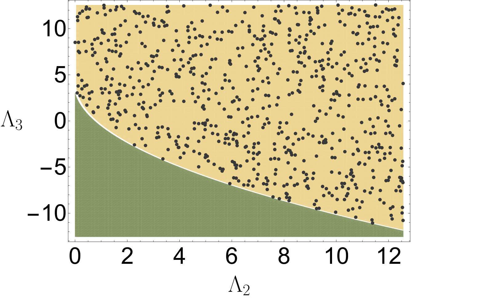
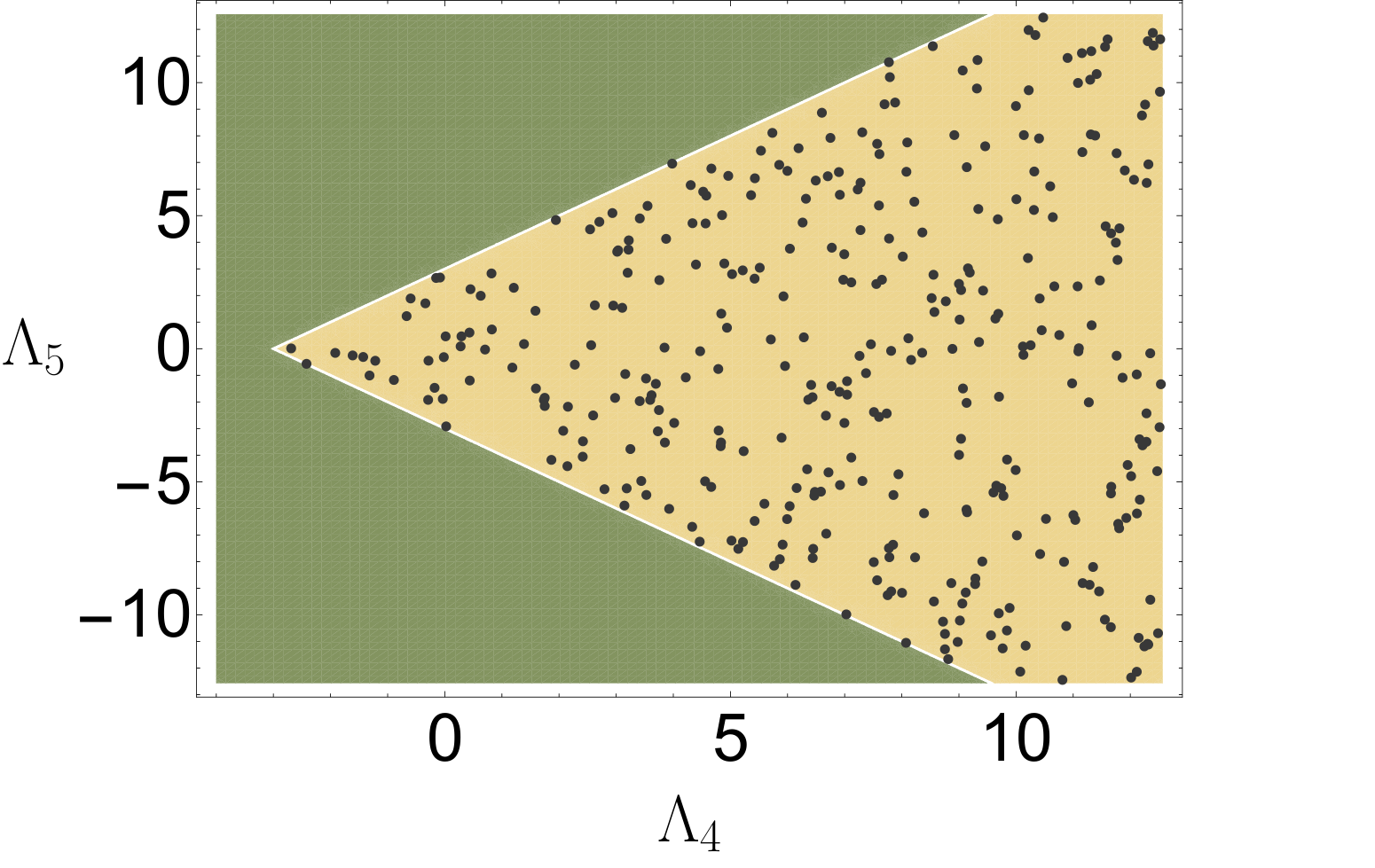
The green region is excluded by the analytic constraints of Eq. (6). The yellow region is allowed. Black dots are those points from the numerical scan which were approved by the package BFB. They perfectly agree with the analytical conditions.

It is worth mentioning that Macaulay2 (37) allows one to calculate the resultant not only over a field but also over the ring of integers. This is on average faster because the intermediate polynomial division steps require the division of the coefficients. Within the ring of integers this is effectively done by a modulo operation which is much faster than an actual division. The computation time varied from 3 hours to 8 hours per parameter space point. Almost the whole time was spent for the calculation of the resultant. We also observed a strong dependence of the calculation time on the complexity of the input parameters: simpler coefficients such as $1/10$ would result in a faster calculation than coefficients like $743/999$.

According to (12), for the five-variable version of the IDM, the degree of the characteristic polynomial is equal to $N_{Q}=5\times 3^{4}=405$. Hence the initial parameters will approximately be raised to this total power making the resulting numerator and denominator a huge number which cannot be stored in CPU registers. For instance, with $\Lambda_{1}=\Lambda_{2}=\Lambda_{3}=1$, $\Lambda_{4}=9.01587$ and $\Lambda_{5}=-10.2132$ the largest coefficient of the characteristic polynomial is

$$\approx 3.452\cdot 10^{1137}\,.$$

(41)

Thus, special libraries for integer manipulation, which emulate the CPU’s arithmetic logic unit, have to be used. The runtime of the remaining algorithm, after the calculation of the characteristic polynomial, is negligible. For the above parameter point, calculating and testing all H-eigenvalues takes no longer than $3$ seconds.

Checking that scalar potentials are BFB is a notoriously difficult problem, which impedes efficient exploration of many models with extended scalar sectors. Analytical BFB conditions are known only in special and rather simple cases. For example, in models with three Higgs doublets the BFB conditions remain unknown beyond the few cases with large symmetry groups.

In this work we presented and developed a novel approach to establishing the BFB conditions of generic polynomial scalar potentials, which, to our best knowledge, was briefly mentioned only in [12] and was not pursued any further by the HEP community. The method relies on certain unconventional mathematical methods such as the theory of resultants and the spectral theory of tensors. In this approach, the BFB conditions are equivalent to calculating a well defined characteristic polynomial and checking that its real roots satisfy certain conditions. We described an explicit algorithm of calculating the characteristic polynomial and illustrated it with two elementary cases, where all calculations can be done manually. We also implemented the algorithm in a Mathematica package BFB [28] which is publicly available at GitHub. We validated its performance with the case of the Inert Doublet Model, for which the conditions are known analytically, and we found perfect agreement.

Unfortunately, we have not yet produced ready-to-use analytical results for other, more complicated cases, where the BFB conditions are at present unknown. This is in part due to the intrinsic complexity of the problem: it is NP-hard and the computation time grows exponentially with the input information. However, we also believe that our current implementation is not the most optimal one, and we hope that it can be dramatically improved in the future. Since the approach is novel, we call for a community effort in optimizing this approach.

The algorithm presented in this work is capable of constructing BFB constraints for any Higgs potential. The bottleneck of runtime is the calculation of the characteristic polynomial. We see four possible improvements that may increase the speed drastically.

First, the current implementation of BFB (28) uses no parallelization even though there is great potential to do so. This is mainly because the whole calculation of the resultant is outsourced to the computer algebra system Macaulay2 (37). There are two critical algorithms that may be subject to improvement: the calculation of the Gröbner bases and the calculation of the resultant. Both of them are under steady investigation of the mathematical community. For Gröbner bases, there are Faugére’s algorithms F4 (41) and F5 (42) both of which are highly parallelizable. Macaulay2 includes already four different algorithms for the calculation of the resultant. The algorithm presented in Section 3.3 from (35, theorem 3.4) is one of them. Part of it is the calculation of the intermediate matrices $M_{i}$. Currently, the elements are obtained in a linear way on one CPU only. However, each row can be calculated independently. For the IDM test of Section 4.4, $M_{1}$ already has $81$ rows, so here is a huge potential for parallelization. Also, the calculation of the basis of the quotient ring is a simple scan through low degree polynomials and can be distributed over any number of cores. Macaulay2 implements also the classic algorithm by Macaulay (34). It is less space efficient but may be more time efficient when it comes to the calculation of resultants of polynomials with many variables. Furthermore, Macaulay2 implements a variation of these two algorithms that makes use of polynomial interpolation (see for instance (43) and (44)).

Second, as one can probably already conclude, not only the possibility of parallelization may speed up the process of resultant calculations, but also the choice of the respective algorithm. There is a multitude of publications on this topic. Depending on the specific form of the input polynomials there might exist much faster algorithms than the presented one. For instance, Macaulay proposed a modified version of his algorithm that can be used if all polynomials share the same degree (45). This is applicable to the current case of Higgs potential boundedness and should definitely be tested. It is this approach that might bypass the NP-hardness (33) of resultant calculations for Higgs potential boundedness.

Third, the scalar potentials we encounter are gauge invariant, and this implies a certain redundancy when writing them in terms of real fields. For example, for the IDM test of Section 4.4, we used the $\mathrm{SU}(2)$ symmetry of the Higgs potential to reduce the number of variables from 8 to 5. It is plausible that additional symmetries of other multi-Higgs models can be exploited in a similar way. Furthermore, since the BFB check can be performed in any basis, one may take advantage of the basis-change freedom to switch to a basis that is more convenient. This may result in a further reduction of variables or parameters. Another symmetry driven approach is the usage of E-eigenvalues (31), which are, unlike H-eigenvalues, invariant under orthogonal transformations. A short discussion of the implications with respect to Higgs potential boundedness can be found in (40).

Lastly, when performing the scans of the parameter space, one can use the ring of integers instead of a field of numbers for the polynomial coefficients. As we saw with the IDM example in Section 4.4, this option changes the runtime. Rational numbers $\mathbb{Q}$ might be the worst choice because they incorporate an inefficient division algorithm (finding greatest common divisors etc.) and have a bad scaling with powers (numerator and denominator can get very large). Integers $\mathbb{Z}$ are more efficient when it comes to the used division operations (modulo operations) but still possess a bad scaling with powers. Macaulay2 only allows for these two options. The field of real numbers $\mathbb{R}$ may be an intermediate solution that trades accuracy for runtime. The division algorithm is not as fast as for integers but calculations of powers are faster and more space efficient (floating point numbers store powers separately). Currently there exists no implementation of resultant algorithms that work with both analytic parameters and real numbers. There is a working framework called MARS (46) that can handle the calculation of the resultant numerically. It is possible to perform a scan over a bounded range of values for the eigenvalues $\lambda$ and test for the numerical vanishing of the resultant. This is numerically unstable though, since the resultant is in general a high-degree polynomial in $\lambda$ and accuracy will play an important role here. Nevertheless, this is a feasible approach.

The long term goal is to have an algorithm that can produce the analytic form of the characteristic polynomial for various Higgs potentials. It is true that computing this polynomial in a specific model, for example, in 3HDM, even after parallelization and optimizaiton may require much computer time. However, once the characteristic polynomial is calculated in its full analytic form, it can be published and distributed, and it can be readily used for all subsequent checks of BFB conditions in this model. Such “mining of characteristic polynomials” is definitely worthy of extra efforts.

Acknowledgments. We are grateful to Kristjan Kannike for his valuable comments. We also want to thank Sven Caspart for the insightful discussions about algebraic geometry. I.P.I. was supported by the Portuguese Fundação para a Ciência e a Tecnologia (FCT) through the Investigator contract IF/00989/2014/CP1214/CT0004 under the IF2014 Program and in part by contracts UID/FIS/00777/2013 and CERN/FIS-NUC/0010/2015, which are partially funded through POCTI, COMPETE, QREN, and the European Union. M.K. and M.M. acknowledge financial support from the DFG project “Precision Calculations in the Higgs Sector — Paving the Way to the New Physics Landscape” (ID: MU 3138/1-1).

References

- (1) ATLAS collaboration, G. Aad et al., Observation of a new particle in the search for the Standard Model Higgs boson with the ATLAS detector at the LHC, Phys. Lett. B716 (2012) 1–29, [1207.7214].
- (2) CMS collaboration, S. Chatrchyan et al., Observation of a new boson at a mass of 125 GeV with the CMS experiment at the LHC, Phys. Lett. B716 (2012) 30–61, [1207.7235].
- (3) I. P. Ivanov, Building and testing models with extended Higgs sectors, Prog. Part. Nucl. Phys. 95 (2017) 160–208, [1702.03776].
- (4) M. Maniatis, A. von Manteuffel, O. Nachtmann and F. Nagel, Stability and symmetry breaking in the general two-Higgs-doublet model, Eur. Phys. J. C48 (2006) 805–823, [hep-ph/0605184].
- (5) N. G. Deshpande and E. Ma, Pattern of symmetry breaking with two higgs doublets, Phys. Rev. D 18 (Oct, 1978) 2574–2576.
- (6) F. Nagel, New aspects of gauge-boson couplings and the Higgs sector, Ph.D. thesis, Heidelberg U., 2004.
- (7) I. P. Ivanov, Two-Higgs-doublet model from the group-theoretic perspective, Phys. Lett. B632 (2006) 360–365, [hep-ph/0507132].
- (8) C. C. Nishi, CP violation conditions in N-Higgs-doublet potentials, Phys. Rev. D74 (2006) 036003, [hep-ph/0605153].
- (9) I. P. Ivanov, Minkowski space structure of the Higgs potential in 2HDM, Phys. Rev. D75 (2007) 035001, [hep-ph/0609018].
- (10) K. Kannike, Vacuum Stability Conditions From Copositivity Criteria, Eur. Phys. J. C72 (2012) 2093, [1205.3781].
- (11) J. Chakrabortty, P. Konar and T. Mondal, Copositive Criteria and Boundedness of the Scalar Potential, Phys. Rev. D89 (2014) 095008, [1311.5666].
- (12) K. Kannike, Vacuum Stability of a General Scalar Potential of a Few Fields, Eur. Phys. J. C76 (2016) 324, [1603.02680].
- (13) C. C. Nishi, The Structure of potentials with N Higgs doublets, Phys. Rev. D76 (2007) 055013, [0706.2685].
- (14) I. P. Ivanov, Properties of the general NHDM. II. Higgs potential and its symmetries, JHEP 07 (2010) 020, [1004.1802].
- (15) M. Maniatis and O. Nachtmann, Stability and symmetry breaking in the general three-Higgs-doublet model, JHEP 02 (2015) 058, [1408.6833].
- (16) M. Maniatis and O. Nachtmann, Stability and symmetry breaking in the general -Higgs-doublet model, Phys. Rev. D92 (2015) 075017, [1504.01736].
- (17) J. Kim, General Method for Analyzing Higgs Potentials, Nucl. Phys. B196 (1982) 285–300.
- (18) J. Kim, SU() Higgs Problem With Adjoint Representation and Michel’s Conjecture, Nucl. Phys. B197 (1982) 174–188.
- (19) M. Abud and G. Sartori, The Geometry of Orbit Space and Natural Minima of Higgs Potentials, Phys. Lett. 104B (1981) 147–152.
- (20) M. Abud and G. Sartori, The Geometry of Spontaneous Symmetry Breaking, Annals Phys. 150 (1983) 307.
- (21) G. C. Branco, J. M. Gerard and W. Grimus, Geometrical T Violation, Phys. Lett. 136B (1984) 383–386.
- (22) K. G. Klimenko, On Necessary and Sufficient Conditions for Some Higgs Potentials to Be Bounded From Below, Theor. Math. Phys. 62 (1985) 58–65.
- (23) R. de Adelhart Toorop, F. Bazzocchi, L. Merlo and A. Paris, Constraining Flavour Symmetries At The EW Scale I: The A4 Higgs Potential, JHEP 03 (2011) 035, [1012.1791].
- (24) A. Degee, I. P. Ivanov and V. Keus, Geometric minimization of highly symmetric potentials, JHEP 02 (2013) 125, [1211.4989].
- (25) M. Maniatis, D. Mehta and C. M. Reyes, Stability and symmetry breaking in a three-Higgs-doublet model with lepton family symmetry O(2), Phys. Rev. D92 (2015) 035017, [1503.05948].
- (26) M. Heikinheimo, K. Kannike, F. Lyonnet, M. Raidal, K. Tuominen and H. Veermäe, Vacuum Stability and Perturbativity of SU(3) Scalars, JHEP 10 (2017) 014, [1707.08980].
- (27) P. M. Ferreira, I. P. Ivanov, E. Jiménez, R. Pasechnik and H. Serôdio, CP4 miracle: shaping Yukawa sector with CP symmetry of order four, JHEP 01 (2018) 065, [1711.02042].
- (28) M. Köpke, “BFB, a Mathematica package to check boundedness of general Higgs potentials.” Available at https://git.io/vFQvi, 2017.
- (29) L.-H. Lim, Singular Values and Eigenvalues of Tensors: A Variational Approach, ArXiv Mathematics e-prints (July, 2006) , [math/0607648].
- (30) L. Qi, Eigenvalues of a real supersymmetric tensor, Journal of Symbolic Computation 40 (2005) 1302 – 1324.
- (31) L. Qi, The Spectral Theory of Tensors (Rough Version), ArXiv e-prints (Jan., 2012) , [1201.3424].
- (32) L. Qi and Z. Luo, Tensor Analysis: Spectral Theory and Special Tensors. Other Titles in Applied Mathematics. Society for Industrial and Applied Mathematics, 2017.
- (33) B. Grenet, P. Koiran and N. Portier, The Multivariate Resultant Is NP-hard in Any Characteristic, Lecture Notes in Computer Science 6281 (2010) 477, [0912.2607].
- (34) F. S. Macaulay, Some formulæ in elimination, Proceedings of the London Mathematical Society s1-35 (1902) 3–27.
- (35) D. A. Cox, J. B. Little and D. O’Shea, Using algebraic geometry. Graduate texts in mathematics; 185. Springer, New York, 1998.
- (36) Wolfram Research, Inc., “Mathematica, Version 11.2.”
- (37) D. R. Grayson and M. E. Stillman, “Macaulay2, a software system for research in algebraic geometry.” Available at http://www.math.uiuc.edu/Macaulay2/.
- (38) G. Staglianò, “Macaulay2 package Resultants: Resultants, discriminants, and Chow forms. Version 1.0.” Available at http://www2.macaulay2.com/Macaulay2/doc/Macaulay2-1.10/share/doc/Macaulay2/Resultants/html/, 2017.
- (39) T. Zell, “Mathoverflow - existence of a real-valued solution to system of multivariate polynomial equations.” Available at https://mathoverflow.net/a/66870/69288, 2017.
- (40) M. Köpke, “Investigation of the GCP Structure of Three-Higgs-Doublet Models and a General Method to Derive Boundedness Constraints for Multi-Higgs Potentials.” Available at http://www.teco.edu/~koepke/mastersthesis.pdf, Master’s thesis, Karlsruhe Institute of Technology, 2018.
- (41) J.-C. Faugére, A new efficient algorithm for computing gröbner bases (f4), Journal of Pure and Applied Algebra 139 (1999) 61 – 88.
- (42) J.-C. Faugére, A new efficient algorithm for computing gröbner bases without reduction to zero (f5), in Proceedings of the 2002 International Symposium on Symbolic and Algebraic Computation, ISSAC ’02, (New York, NY, USA), pp. 75–83, ACM, 2002, DOI.
- (43) D. Manocha, Efficient algorithms for multipolynomial resultant, The Computer Journal 36 (1993) 485–496.
- (44) D. Manocha and J. F. Canny, Multipolynomial resultant algorithms, Journal of Symbolic Computation 15 (1993) 99 – 122.
- (45) F. S. Macaulay, Note on the resultant of a number of polynomials of the same degree, Proceedings of the London Mathematical Society s2-21 (1923) 14–21.
- (46) A. Wallack, D. Manocha and I. Emiris, “Mars, maple/matlab/c resultant-based solver.” Available at http://gamma.cs.unc.edu/MARS/, 2017.