Detection significance of Baryon Acoustic Oscillations peaks in galaxy and quasar clustering
Abstract
We compare our analysis of the Baryon Acoustic Oscillations (BAO) feature in the correlation functions of SDSS BOSS DR12 LOWZ and CMASS galaxy samples with the findings of Cuesta et al. (2016). Using subsets of the data we obtain an empirical estimate of the errors on the correlation functions which are in agreement with the simulated errors of Cuesta et al. (2016). We find that the significance of BAO detection is the quantity most sensitive to the choice of the fitting range with the CMASS value decreasing from to as the fitting range is reduced. Although our measurements of are in agreement with those of Cuesta et al. (2016), we note that their CMASS (LOWZ ) detection significance reduces to () in fits with their diagonal covariance terms only. We extend our BAO analysis to higher redshifts by fitting to the weighted mean of 2QDESp, SDSS DR5 UNIFORM, 2QZ and 2SLAQ quasar correlation functions, obtaining a measurement compared to achieved by eBOSS DR14. Unlike for the LRG surveys, the larger error on quasar correlation functions implies a smaller role for nuisance parameters (accounting for scale-dependent clustering) in providing a good fit to the fiducial CDM model. Again using only the error bars of Ata et al. (2018) and ignoring any off-diagonal covariance matrix terms, we find that the eBOSS peak significance reduces from 2.8 to . We conclude that for both LRGs and quasars, the reported BAO peak significances from the SDSS surveys depend sensitively on the accuracy of the covariance matrix at large separations.
Keywords:
cosmology: observations, distance scale, large-scale structure, BAO, QSO1 Introduction
The determination of the expansion history of the universe is currently one of the primary goals of observational cosmology. The late-time transition of the expansion rate of the universe from a deceleration to a phase of acceleration (e.g. based on observational evidence from supernovae; Riess et al. 1998; Perlmutter et al. 1999) in particular, remains one of the most puzzling problems in modern physics. Investigating this problem and exploring the nature of Dark Energy (a hypothetical cause of the accelerated expansion rate of the universe (Peebles & Ratra, 2003), within the framework of CDM, the current standard cosmological model), have driven efforts to obtain robust and high precision measurements of the cosmological expansion rate. To this end, a great interest was sparked in exploiting large galaxy redshift surveys in order to constrain the distance-redshift relation across a wide range of redshifts, making use of the Baryon Acoustic Oscillation (BAO) feature in the clustering of galaxies (e.g. Shanks 1985; Blake & Glazebrook 2003; Linder 2003; Seo & Eisenstein 2003; Matsubara 2004; Glazebrook & Blake 2005; Dolney et al. 2006; Sánchez et al. 2008).
A measurement of the BAO signature in the monopole two point correlation function of the “Constant Stellar Mass” (CMASS) and the low-redshift (LOWZ) galaxy samples from the Data Release 12 (DR12; Alam et al. 2015) of the SDSS BOSS survey was presented by Cuesta et al. (2016). The CMASS and LOWZ samples are extensions to previous SDSS LRG samples.
Here, we first present the results of our independent measurement of the BAO feature in the DR12 CMASS and LOWZ samples. This is followed by a comparison to results of Cuesta et al. (2016) providing an independent verification of the applied methodology, placing particular focus on the uncertainties on the correlation functions. Cuesta et al. (2016) obtained an estimate of the uncertainties based on the covariance matrix of BOSS DR12 simulated QPM mocks (White et al., 2014). In this study, we divide the data into subsamples upon which measurements of the correlation function are performed, giving an empirical estimate of the uncertainty on the mean correlation function. Furthermore, we investigate certain aspects of the fitting procedure commonly implemented in BAO analysis studies. These include the extent of the role played by the nuisance fitting parameters in providing a good fit; effects of the choice of the fitting range on the results and a comparison between fits using the full BOSS DR12 QPM covariance matrices and their diagonal elements only. Here our main goal is to investigate the robustness of the BAO peak detection significance to variations in different aspects of the fitting procedure. Note that in this work we do not attempt to perform reconstruction and hence we simply draw comparison with the pre-reconstruction results throughout.
At higher redshifts, BAO have also been detected in the Lyman-alpha forest in the BOSS quasar survey at (Slosar et al. 2013; Delubac et al. 2015). As originally suggested by Sawangwit et al. (2012), it is also possible to make accurate BAO measurements in the range using quasars as direct tracers of the matter distribution. The eBOSS survey (Dawson et al., 2016) is therefore making BAO measurements via quasars using them both directly as tracers and via the Lyman-alpha forest. Here we shall use the SDSS DR5 (Ross et al., 2009), 2SLAQ (Croom et al., 2009), 2QZ (Croom et al., 2004) and 2QDES pilot (Chehade et al., 2016) surveys to determine the level of accuracy to which the BAO scale can be measured by the previous generation of quasar surveys used as direct tracers in the redshift range. Furthermore, we combine our results with those of Ata et al. (2018) who performed BAO analysis on the eBOSS DR14 quasar sample in the same redshift range, obtaining a BAO distance measurement based on the combination of these samples.
The layout of this paper is as follows: Section 2 contains a brief description of the galaxy samples along with the basic properties of the selected subsamples. In Section 3 we present a description of the relevant methodology involved in measuring the correlation function, error analysis and the fitting procedure. This is followed by a presentation and discussion of our results and a comparison of our findings with those of Cuesta et al. (2016) in Section 4. In Section 5 we provide a description of the quasar samples used in our high redshift BAO analysis, followed by an outline of our applied methodology in section 6. We present the results of our QSO BAO analysis in section 7, along with the cosmological distance constraints obtained from our QSO and LRG measurements, comparing our findings with the predictions of Planck Collaboration et al. (2016). Finally, we conclude this work by providing a summary of our findings in Section 8.
2 Datasets
In this study we first use a set of 777,202 galaxies in the redshift range from the BOSS DR12 CMASS sample, with an effective redshift of 0.57, and 361,762 galaxies in the redshift range from the DR12 LOWZ sample, with an effective redshift of 0.32. The CMASS and LOWZ samples have been limited to magnitudes of and respectively. Full details of the target selection criteria can be found in Reid et al. (2016) and the treatment of systematics and the relevant corrections is discussed in Ross et al. (2017). In accordance with Cuesta et al. (2016), the samples, mocks and random datasets were obtained from the DR12 database11 1 https://data.sdss.org/sas/dr12/boss/lss/. The redshift distributions , of the galaxies in the DR12 CMASS and LOWZ samples are displayed in Fig. 1.

In order to obtain an empirical estimate of the uncertainties on the correlation functions, the CMASS sample is subsetted into five fields (subsamples) of equal size covering an overall area of 8487.77 , about of the total effective sample area (9376.09 ). The LOWZ sample is similarly divided into five equally sized fields covering 7294.87 , roughly of the total sample area (8337.47 ). Initially, dividing the samples into five fields was deemed sufficient in order to produce an estimate of the uncertainties to a reasonable degree of accuracy. However, as demonstrated in later sections, the precision of the empirical estimate of uncertainties can be further improved by using a larger number of subsamples. The positions of all selected fields are illustrated in Fig. 2, with Table 1 providing a description of the basic properties of the selected fields. Once the correlation function for each field is obtained, a mean correlation function is calculated and is taken to represent the correlation function of the sample, using the standard error on the mean as an estimate of the uncertainty.


| CMASS | ||||
|---|---|---|---|---|
| Field | Ra° | Dec° | Area () | Number of galaxies |
| 1 | >185 | >27 | 1703 | 142,636 |
| 2 | <185 | >27 | 1686 | 141,706 |
| 3 | >185 | <27 | 1699 | 141,847 |
| 4 | 119-185 | <27 | 1698 | 137,891 |
| 5 | 350-45.5 | >-11 | 1701 | 144,820 |
| LOWZ | ||||
| Field | Ra° | Dec° | Area () | Number of galaxies |
| 1 | >185 | >27 | 1447 | 61,319 |
| 2 | <185 | >27 | 1453 | 63,109 |
| 3 | >185 | <27 | 1474 | 61,605 |
| 4 | <185 | <27 | 1463 | 63,431 |
| 5 | 357-45.5 | >-11 | 1459 | 68,057 |
In our analysis up to Section 5, we assume the same fiducial cosmology as Cuesta et al. (2016) with , , , , , , , and . The fiducial distances to and (the effective redshifts of our samples), based on our assumed cosmology are presented in Table 2.
| (Mpc) | (Mpc) | (km s-1 Mpc-1) | (Mpc) | (Mpc) | (km s-1 Mpc-1) | (Mpc) |
| 147.10 | 962.43 | 82.142 | 1235.28 | 1351.13 | 94.753 | 2009.55 |
3 Methodology
3.1 Measuring the Correlation Function
The monopole two-point correlation function (in redshift-space), , is calculated for each individual field using the CUTE22 2 http://members.ift.uam-csic.es/dmonge/CUTE.html algorithm described by Alonso (2012).
To perform the measurement of the correlation function we make use of the Landy-Szalay estimator (Landy & Szalay, 1993),
| (1) |
where , and are data-data, data-random and random-random pair-counts respectively.
In our analysis we make use of the BOSS DR12 FKP-weighted (Feldman et al., 1994) randoms, and in accordance with Reid et al. (2016), apply a weighting of to the galaxies. A full description of the constituents of is presented in Reid et al. (2016); in short, this weight consists of three terms which account for effects of angular systematics, fibre collisions and redshift failures. In order to facilitate direct comparison with the findings of Cuesta et al. (2016), we sum our pair counts into 25 bins of width Mpc in our calculation of the correlation functions, covering the range of Mpc in redshift space.
3.2 Error Analysis
Following the procedure proposed by Norberg et al. (2009), the bootstrap resampling method is used to provide an estimate of the errors on the mean correlation functions of our CMASS and LOWZ samples. In total we generate resamplings and obtain the mean correlation function of these resamplings. As demonstrated by Norberg et al. (2009), an oversampling factor of 3 appears to be optimal in improving the bootstrap recipe. Hence we calculate the mean correlation function of each resampling, , based on the correlation functions of randomly selected subvolumes (with replacement), from the original subvolumes defined in Section 2 for the CMASS and LOWZ samples.
A second set of errors are determined for the mean correlation functions of our samples, simply based on obtaining the standard errors on the mean. This is done using,
| (2) |
where is the standard deviation normalized to (as is obtained from the same dataset reducing the number of degrees of freedom by one); is the number of subvolumes in each sample (i.e. 5); is the correlation function of the th subvolume, and is the mean correlation function of the sample.
A comparison of the estimated errors from these two different methods and the errors found by Cuesta et al. (2016) based on the covariance matrix of the DR12 QPM mocks is presented in Section 4.2.
3.3 Fitting the Correlation Function
To fit the correlation functions we follow a procedure based on the methods described in Xu et al. (2012) and Anderson et al. (2012). We present a brief description of these techniques in this section.
We use a fitting model of the form
| (3) |
where is defined in equation 7, is a constant term allowing for any unknown large-scale bias and is given by
| (4) |
where are nuisance parameters. The term is included in order to marginalise over broad-band effects due to redshift-space distortions and scale-dependent bias as well as any errors made in our assumption of the fiducial cosmology. The form of the term was chosen by Xu et al. (2012) due to its simplicity and was further justified in that work by comparing it to various alternatives and demonstrating that it performs optimally in providing a good fit. We can obtain distance constraints by finding the optimum value of the scale dilation parameter . This parameter provides a measure of any isotropic shifts in the position of the BAO peak in the data compared to the fiducial model, due to non-linear structure growth. This term is defined as
| (5) |
where is the redshift, is the sound horizon at the drag epoch and denotes the fiducial values (given in Table 2). An () indicates that the BAO peak in the observed data is located at a smaller (larger) scale compared to the peak in the model. The approximate volume-averaged distance to redshift is
| (6) |
where is the angular diameter distance and is the Hubble parameter at redshift . This “distance” is proportional to the volume-averaged dilation factors (Ballinger et al., 1996) in the redshift and angular directions at a redshift .
The model correlation function in equation (3), , is given by
| (7) |
where the Gaussian term is added to damp the oscillatory transform kernel at high-. Here we set Mpc, which is small enough as to not cause significant damping effects at our scales of interest.
The template power spectrum is given by
| (8) |
where is the linear power spectrum at (generated using CAMB33 3 http://cosmologist.info/camb/; Lewis et al. 2000) and is the power spectrum with the BAO feature removed as described in Eisenstein & Hu (1998). The term damps the BAO features in , accounting for the effects of non-linear structure evolution. Here we set Mpc.
The best fit values of the , , and fitting parameters in equation 3 are determined using the scipy.optimize.curve_fit module in Python which makes use of the Levenberg-Marquardt algorithm. To obtain the optimum value of we compute the goodness-of-fit indicator for fits obtained from shifting the model in the range with intervals of , taking the value of which corresponds to the minimum , ().
The function is given by
| (9) |
where is the observed correlation function, is the best fit model at each and is the BOSS DR12 covariance matrix obtained from 1000 simulated QPM mocks.
In this study we investigate potential effects on the measured value of and its uncertainty based on fitting the data across various ranges, using the complete model with and without the nuisance parameters. Furthermore, by comparing the vs. curves from fitting the and models (the latter is obtained by setting the term in the model correlation function ), we obtain a measure of the significance at which the BAO signature is detected in the data. Here .
To obtain an estimate of the uncertainty in , we assume a Gaussian form for the probability distribution of ,
| (10) |
where the denominator is a normalization factor ensuring the distribution integrates to unity. In effect is the probability that the acoustic scale , based on the distribution obtained from comparing the model (equation (3) with ), to our observed correlation function . We then calculate the standard deviation of our probability distribution which serves as an estimate of the uncertainty in :
| (11) |
here represents the mean of the distribution given by:
| (12) |
and
| (13) |
The estimated uncertainty obtained from this method is equivalent to the value given by the curve at the level (see Fig. 7(a)).
4 Results and Discussion
The correlation functions of the individual fields for the LOWZ and CMASS samples along with the corresponding mean correlation functions are displayed in Fig. 3. We note that there is quite a wide variation in these correlation functions with e.g. field 4 for CMASS showing high values at Mpc. In the following sections we compare our measurement of the mean correlation functions with the measurements of Cuesta et al. (2016), perform fitting to the mean correlation functions and analyse various aspects of the fitting procedure. Furthermore, we obtain measurements of based on our measured position of the BAO peak.


4.1 Comparison with Cuesta et al. (2016)
Fig. 4 shows a comparison between our mean correlation functions and the correlation functions obtained by Cuesta et al. (2016) for the DR12 LOWZ and CMASS samples. We find that our measured correlation functions are in excellent agreement with those presented in Cuesta et al. (2016) and we observe no significant changes when we replace the BOSS DR12 randoms with randoms generated by CUTE. Furthermore, we observe no significant variations when we do not apply any weights to the data or randoms. This outcome is however expected due to the high completeness of and for the CMASS and LOWZ samples respectively (Reid et al., 2016, see Fig. 8 of).


.
4.2 Error Analysis Results
This section contains a comparison between our two measures of uncertainties (standard error and bootstrap resampling) on the mean correlation functions of the LOWZ and CMASS samples. Here we also include the bootstrap uncertainties based on dividing the CMASS sample into 30 subsamples (see figures in Appendix A). We distinguish between the two bootstrap uncertainties using the labels ‘CMASS 5’ and ‘CMASS 30’. More importantly comparisons are drawn between our measured empirical errors and errors obtained from simulations presented in Cuesta et al. (2016) for the correlation functions of the LOWZ and CMASS samples. In order to account for the fact that our selected fields do not cover the entire sample area, when comparing our results with those from Cuesta et al. (2016) we scale our measured errors by the square root of the ratio of the total coverage area of our fields to the total sample area.
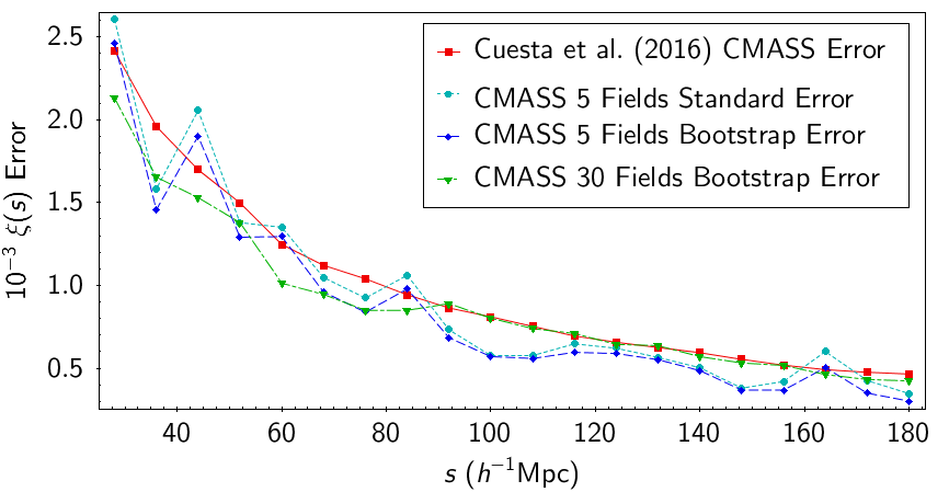


As shown in Figs. 5(a) and 5(b), we find a good agreement between the standard error and bootstrap error estimates for both samples. Fig. 5(a) shows that at our main scale of interest (in the vicinity of the Mpc bin where the BAO peak lies), our results for the 5 fields CMASS sample also appear to be in reasonable agreement with the errors presented by Cuesta et al. (2016). Furthermore, our 30 fields bootstrap uncertainties appear to be in excellent agreement with those from Cuesta et al. (2016) at scales larger than Mpc. To provide a quantitative demonstration of the level agreement between the errors from Cuesta et al. (2016) and the simple case of standard errors obtained from 5 fields, we make use of the fractional error in the error, given by (Squires, 2001). Here is the number of measurements (in our case 5), giving a fractional error in the error of . Fig. 5(c) shows the ratio of our measured standard error to the errors presented by Cuesta et al. (2016) for the CMASS sample with the error bars being the error on our measured standard error. We can see that at the Mpc bin this ratio is which is consistent with unity within the error bars, and the general agreement between the errors is an indication that the QPM mocks reproduce an accurate representation of the data. As shown in Fig. 5(d) however, in the case of the LOWZ sample the ratio between the two errors varies to a greater extent as a function of scale, with the discrepancy between the two errors being larger around the BAO scale. This indicates that the errors presented by Cuesta et al. (2016) do not appear to be underestimated in this region.
4.3 Data Fitting Results
The best-fit values of obtained from fitting the data with various models, across 20 bins, with centres in the range Mpc are summarised in Table 344 4 Note that we place the main focus of our analysis on the results corresponding to this fitting range in order to match the fitting range chosen in Cuesta et al. (2016), allowing for direct comparison of the results. As discussed in Section 3.3, when fitting the correlation functions we use the BOSS DR12 covariance matrix used in the analysis of Cuesta et al. (2016).. The pre-reconstruction best fit values of from Cuesta et al. (2016) are included in this table for comparison. Here, ‘’ refers to values obtained from fitting to the mean correlation functions of the LOWZ and CMASS samples, with errors given by the procedure described in Section 3.3. The ‘5-fields ’ values in this table are obtained by fitting to the correlation functions of each field individually resulting in 5 measurements of (these are presented in Table 4), and calculating the mean and standard error of these measurements. When fitting to correlation functions of individual fields we scale the BOSS DR12 covariance matrix by a factor of 5.
As shown in Table 3, we find that our measured ‘5-fields ’ values are in good agreement with our overall values of . This demonstrates the robustness of the implemented fitting procedure in producing an accurate measurement of the position of the BAO peak. Furthermore, when comparing the results corresponding to fits with the complete model, we find that for both CMASS and LOWZ samples, our measured values of are in agreement with the measurement presented by Cuesta et al. (2016), with the errors on being similar in size.
| This Work | Model | Significance | -ratio | 5-fields | ||
| CMASS | 14.9/15 | |||||
| 28.5/18 | ||||||
| LOWZ | 15.5/15 | |||||
| 45.5/18 | ||||||
| Cuesta et al. (2016) | Model | Significance | ||||
| CMASS | 12/15 | |||||
| LOWZ | 13/15 |
| This Work | Field | Model | Significance | ||
|---|---|---|---|---|---|
| 1 | 14.5/15 | ||||
| 21.7/18 | |||||
| 2 | 16.2/15 | ||||
| 21.1/18 | |||||
| CMASS | 3 | 12.6/15 | |||
| 12.2/18 | |||||
| 4 | 13.5/15 | ||||
| 29.7/18 | |||||
| 5 | 10.8/15 | ||||
| 12.2/18 | |||||
| 1 | 34.6/15 | ||||
| 35.3/18 | |||||
| 2 | 23.7/15 | ||||
| 33.8/18 | |||||
| LOWZ | 3 | 17.0/15 | |||
| 16.3/18 | |||||
| 4 | 22.3/15 | ||||
| 26.0/18 | |||||
| 5 | 18.2/15 | ||||
| 43.5/18 |
We find the values of measured for the individual fields in Table 4 to be in general agreement with the measurements of from Cuesta et al. 2016. In cases where there appears to be a divergence between the measurements, (for instance our result of fitting the correlation function of field 4 in the CMASS sample with the complete model appears to be away from the value of measured by Cuesta et al. 2016), the dependency seems to be due to the shape of the BAO peak (which in this case appears to be relatively flat, as seen in Fig. 3(a)). However, as the ‘5-fields ’ values are in agreement with the measurements of from the mean correlation functions, these effects seem to cancel out when we take the average over the 5 fields, even given our relatively small number of subsamples.
The performance of the two models in fitting the correlation functions (given by the goodness of fit indicator) also appear to vary largely depending on the shape of the correlation function. However, with the exception of certain fields (for instance field 3 of both CMASS and LOWZ samples), the complete model appears to perform better overall in providing good fits. It is important to note however, that the performance of a model in providing a good fit is not necessarily indicative that the correlation function has provided a representative and accurate measurement of , and one should also consider the shape and prominence of the BAO peak in the correlation function itself55 5 In Section 4.5 we discuss how the shape of the curve could also provide a measure of the degree to which we could be confident in our measurement of .. This is exemplified by field 4 in the CMASS sample where the value indicates that the complete model has provided a reasonably good fit to the data but due to the shape of the correlation function (see Fig. 3(a)), an accurate determination of the position of the peak has not been possible. Finally we find that the significance of detection of the peak in the individual fields to be generally lower than the significance of the detection of the peaks in the mean correlation functions of the two samples (as shown in Table 3). This is a further indication of the lack of prominent and well defined peaks in the correlation functions of the individual fields and as shown once again by field 4 in the CMASS sample, a low significance of detection of the peak could also hint towards the potential unreliability of the measured .
4.4 Model Comparison
Fig. 6 shows the results of fitting the mean correlation functions of the CMASS and LOWZ samples with the model, fitted with and without the nuisance parameters, and the model fitted with both and fitting terms. The important role played by the nuisance fitting terms in producing a good fit is highlighted in these plots. This is also demonstrated numerically in Table 3, with the fits without the having increased values indicating the lower quality of fits. We assess the statistic based on the corresponding -value = , which is defined as the probability of obtaining a value at least as extreme as the value obtained, given our null hypothesis : that the data is consistent with the model. In other words, the -value is the probability of obtaining the observed data, under the assumption that the model is correct, and a measure of the significance at which the model is rejected by the data is given by -value.
We note that the visual impression given in Fig. 6(a) is that the CDM model without nuisance parameters for the CMASS sample is rejected at a higher significance than by the () indicated in Table 3. Indeed, when only the diagonal terms of the covariance matrix are used in the fitting, the significance of rejection rises to () (see Table 5). Thus in this case the inclusion of the full covariance matrix causes a large reduction in .
| Full Matrix | Diagonal Elements | ||||||
|---|---|---|---|---|---|---|---|
| Sample | Model | -value | Significance | -value | Significance | ||
| CMASS | |||||||
| LOWZ | |||||||
We then take a more detailed look at how significant the nuisance parameters are in achieving a good fit for the CDM model. Given our two nested fit models, we can make use of the -ratio (see e.g. Gregory 2005) in order to determine whether the use of the more complex model results in a statistically significant improvement in fit quality. The -ratio is given by
| (14) |
Here and refer to the values obtained from fitting the model without the nuisance fitting terms, and by the complete model respectively, and are the degrees of freedom associated with each model. Once the value is obtained we can test the validity of our null hypothesis that the complex model does not provide a significantly better fit than the simple model. Similar to the analysis above, we assess the validity of the null hypothesis based on the -value associated with the resulting statistic.
Based on the values presented in Table 3, for the fitting range Mpc, we obtain values of and for the CMASS and LOWZ samples respectively. In other words our simple model is rejected in favour of the full model by the data, (given that assuming the null hypothesis is correct, i.e. that there is no significant difference between the two models, the probability of obtaining an statistic at least as extreme as the values here by chance are and for the CMASS and LOWZ samples respectively). This means that the inclusion of the nuisance parameters results in a significant improvement to the fit. This is specially true in the case of the LOWZ sample, where as seen in Fig. 6(b), the BAO peak in the correlation function appears flatter in the Mpc range, explaining the strong need for the nuisance parameters at the level of significance indicated by the test.
4.5 Significance of BAO Peak Detection
The curves based on fitting the mean correlation functions of the CMASS and LOWZ samples, with the and models are presented in Fig. 7(a). Here the complete fitting models including the fitting terms are used and , where is the minimum value using the model containing BAO. A comparison of the two models shows that we detect the BAO peak in the data at an level for the LOWZ sample and at for the CMASS sample, in agreement with the findings of Cuesta et al. (2016). Note that we measure the BAO peak detection significance at the best-fit value of given by the model containing BAO. A second test of BAO significance is also captured in Fig. 7(a). For the CMASS sample, it can be seen from the plateau height of the curve (solid blue line), that local maximum lies at a value of above the minimum, meaning that we can apparently be confident in our measured best-fit value of at . For the LOWZ sample, the maximum lies at , indicating that our best fit value of is preferred at by the data. These values are usually taken to indicate that we have obtained well-constrained measurements of in both cases. In the case of the LOWZ sample it can also be seen that the plateau is lower on the left hand side () in comparison to the plateau on the right hand side (). This is once again a consequence of the flatness of the BAO peak in the LOWZ correlation function in the scales of Mpc, as discussed in the previous section.
However, the level of scatter between field-to-field correlation functions around the BAO peak (as shown in Fig. 3), prompts us to caution that and BAO peak significances for CMASS and LOWZ may be over-optimistic. Although, it must be remembered that these significances are calculated after the fitting of nuisance parameters which will clearly remove long-wavelength artefacts that otherwise can add to the noisy impression given by individual fields in Fig. 3.
Another consideration might also involve the anomalously low recorded for our best fit to the CMASS sample with our fiducial plus nuisance parameters model, using the diagonal covariance matrix elements only, compared to using the full matrix, as shown in Table 5 (with the associated plot shown in Fig. 7(b)). In the case of using the diagonal elements, the full noBAO model is also only rejected at (), in comparison to the much higher rejection using the full covariance matrix ().
We find similar results for the LOWZ sample with a reduction from to for our full model using the full and diagonal matrices respectively. We also record a notable reduction in the level of rejection of the noBAO model by the LOWZ data, from () using the full matrix, to a good fit with () using the diagonal elements.
For models with nuisance fitting parameters, using the full covariance matrix appears to increase the significantly compared to using the diagonal terms only. This is opposite to what is seen in other cases such as the fit of the fiducial CDM model where no nuisance parameters are used (see Table 5). This may be due to having both positive and negative fit residuals in the first case and residuals mainly of one sign in the latter case, and a covariance matrix with exclusively positive elements. Given the size of this effect, we perform a further test by replacing the off-diagonal CMASS covariance matrix elements by zero, increasingly far from the diagonal (leaving a ‘band’ matrix). This is motivated by the correlation matrix in Fig. 15 showing that the covariance elements decrease systematically away from the diagonal. We found that maintained when up to the first 14 off-diagonal elements were retained and only increased to when elements 15-20 (indicated in Fig. 15 by the red outline) were included. This effect also appears to be important for assigning the significance of BAO peak detection (as shown in Table 5, reducing the detection significance from to and from to for the CMASS and LOWZ when using the complete fitting model). For the CMASS sample, we observe a similar jump in the significance of peak detection from when only the first 13 off-diagonal elements were included, to once elements 14 and higher are included. We note that here the main contribution to the increase in (and hence the peak detection significance) appears to be from the large increase in the of the noBAO model which rises by , while the of the model containing BAO only rises by 6.5. One can similarly see this in Table 5 with the large increase of in the of the noBAO+ model compared to only for the BAO+ model, as we go from fitting with the diagonal elements only to using the full matrix. The sharp nature of this increase and its marked effect on the significance of model rejection may seem somewhat anomalous, given that one would expect relatively low correlation between points Mpc apart (as shown in Fig. 15). The sensitivity of our results to the inclusion of largely separated off-diagonal covariance matrix elements, demonstrate the importance of the accuracy of covariance matrix estimation.


4.6 The Choice of Fitting Range
In order to investigate the effects of the choice of fitting range on our measured value of and the significance of the detection of the BAO peak, we perform our fitting across 7 different ranges using the model with and without the nuisance fitting terms. We summarise the results in Table 6. It can be seen that the value of and the magnitude of its error are largely insensitive to the choice of the fitting range for the CMASS sample. Slight variations in the value of are observed as the fitting range is varied in the case of the LOWZ sample, however, these values remain consistent within the uncertainties. It can be seen that the quality of the fits produced by the model without the nuisance fitting terms are consistently lower than the fits produced by the complete model across various ranges as shown by the values. The quantity that appears to be most sensitive to the choice of the fitting range is the significance of the detection of the BAO peak in the data. At the two extremes, the significance of the detection of the peak varies from to for the CMASS sample and from to for the LOWZ sample, depending on the choice of the fitting range. Vargas-Magaña et al. (2016) have also examined the effect of the choice of fitting range on the robustness of the BAO peak measurement, reporting noisier results as the lower and upper bounds of the fitting range approach the BAO scale (i.e. Mpc and Mpc respectively), particularly in the former case. This level of variation highlights the importance of providing appropriate justification for the choice of fitting range in studies performing analysis of the BAO feature.
| This Work | Range (Mpc) | Model | Significance | ||
|---|---|---|---|---|---|
| 14.9/15 | |||||
| 28.5/18 | |||||
| 11.9/13 | |||||
| 19.0/16 | |||||
| 11.0/11 | |||||
| 20.6/14 | |||||
| CMASS | 6.6/9 | ||||
| 23.2/12 | |||||
| 6.3/7 | |||||
| 24.7/10 | |||||
| 6.2/5 | |||||
| 28.3/8 | |||||
| 5.6/3 | |||||
| 29.9/6 | |||||
| 15.5/15 | |||||
| 45.5/18 | |||||
| 13.9/13 | |||||
| 49.0/16 | |||||
| 11.7/11 | |||||
| 48.5/14 | |||||
| LOWZ | 7.5/9 | ||||
| 39.0/12 | |||||
| 6.9/7 | |||||
| 43.2/10 | |||||
| 6.7/5 | |||||
| 42.3/8 | |||||
| 5.6/3 | |||||
| 31.3/6 |
4.7 Cosmological Distance Constraints
Using our measured values of and 5-fields presented in Table 3 (for the complete model), and our fiducial distances presented in Table 2, we calculate the volume-averaged distance to redshift , for the LOWZ and CMASS samples. A comparison of our results and the findings of Cuesta et al. (2016) is given in Table 7. As expected given our measurements of , we find our results to be in agreement with those from Cuesta et al. (2016) for both samples. Furthermore, it can be seen that the magnitude of the errors are comparable between the two studies in the case of which is based on the errors on (giving a and percent distance measurement for the LOWZ and CMASS samples respectively), while the ‘5-fields ’ errors are larger due to the larger errors on the 5-fields values.
| Study, Sample | 5-fields | |
|---|---|---|
| (Mpc) | (Mpc) | |
| This work, CMASS | ||
| Cuesta et al. (2016), CMASS Pre-Recon | —– | |
| This work, LOWZ | ||
| Cuesta et al. (2016), LOWZ Pre-Recon | —– |
5 Quasar BAO Analysis
In this section we extend our BAO analysis to higher redshifts by performing isotropic fitting to the combined monopole correlation functions of four quasar samples from the 2dF QSO Redshift Survey (2QZ; Smith et al. 2005), SDSS Data Release 5 (SDSS DR5; Adelman-McCarthy et al. 2007), 2dF-SDSS LRG and QSO survey (2SLAQ; Richards et al. 2005) and the 2dF Quasar Dark Energy Survey pilot (2QDESp; Chehade et al. 2016). In total, these surveys contain quasars in the redshift range. As with the galaxy samples in Section 4.2, we obtain and examine the empirical error of the combined correlation function of the QSO samples, based on the scatter in the data.
In this work, we limit our samples to the range , to allow for direct comparison and combination of our results with those from Ata et al. (2018), who performed BAO analysis on the eBOSS survey of 147,000 quasars in this redshift range. We use the published correlation function of Ata et al. (2018) and re-fit the BAO peak for using the same techniques as for our quasar sample.
5.1 2QZ+SDSS+2SLAQ+2QDESp Datasets
Here we provide a brief summary of the relevant properties of the quasar samples used in our BAO analysis. A more detailed description of these samples can be found in the referenced papers.
The 2QZ sample (Croom et al., 2004) covers a total area of deg2, containing 22,655 QSOs ( quasars deg-2) up to in the magnitude range .
The SDSS DR5 “UNIFORM” sample was constructed by Ross et al. (2009) by taking a subsample of the DR5 quasar catalogue (Schneider et al., 2007). This sample covers an area of deg2, containing 30,239 QSOs ( quasars deg-2), in the redshift range with a magnitude limit of .
The 2SLAQ sample (Croom et al., 2009) covers an area of deg2 containing QSOs ( quasars deg-2) in the redshift range and magnitude range .
The 2QDESp sample (Chehade et al., 2016) covers an area of deg2 in the southern sky, containing QSOs ( quasars deg-2) with magnitudes . The quasars in the sample have a mean redshift of and with of the objects in the sample lying in the range .
As mentioned above, in order to allow direct comparison and combination of our results with the measurements of Ata et al. (2018), we restrict our analysis to objects in the redshift range . This leads to a total number of quasars , of 15,926, 23,386, 4,988 and 7,329 for the 2QZ, SDSS, 2SLAQ and 2QDESp samples respectively. Fig. 8 shows the redshift distribution of the four QSO samples. The weighted mean of the correlation functions of these samples is taken to represent the correlation function of the combined quasar sample (henceforth referred to as the Combined QSO sample), containing 51,629 quasars with a mean redshift of and an effective volume of Gpc3. For comparison the QSO sample of Ata et al. (2018) covers an effective volume of Gpc3, while the original SDSS LRG survey analysed by Eisenstein et al. (2005) covered an effective volume of Gpc3 and the BOSS DR12 LOWZ and CMASS samples analysed by Cuesta et al. (2016) cover effective volumes of Gpc3 and Gpc3 respectively (in all cases we are quoting the effective volumes at Mpc-1).
In this section we assume the same cosmology as Ata et al. (2018) in order to facilitate direct comparison of our results, using a flat CDM cosmology with , , . Although the mean redshift of the Combined QSO sample is , for simplicity and ease of comparison with Ata et al. (2018), we quote our fiducial distance to and present our distance measurement at this redshift, with Mpc and Mpc.
5.2 eBOSS
The eBOSS quasar survey is fully described by Ata et al. (2018), in which BAO measurements were performed based on a sample of 147,000 quasars in the redshift range . With an area of deg2, the quasar sky density of the sample is 72 deg-2. Here we simply use the correlation function from their Fig. 5 along with the QPM error bars.
6 Measuring QSO correlation functions
In this section we summarise the applied methodology in our measurement of the correlation functions of the 2QDESp, 2QZ, 2SLAQ and SDSS QSO samples. We then describe our analysis of the BAO feature in our Combined QSO sample as well as the eBOSS correlation function presented by Ata et al. (2018).
We use the Landy-Szalay estimator (described in Section 3.1), along with random catalogues generated by Chehade et al. (2016), in order to measure the correlation functions of the four QSO samples. The random catalogues are larger than the data for all samples with the exception of SDSS where the random catalogue is larger than the data. To account for effects of photometric and spectroscopic incompleteness, Chehade et al. (2016) have applied appropriate normalisation to these randoms on a field to field basis.
All four correlation functions are calculated using 25 Mpc bins, following the same approach as our measurements of LOWZ and CMASS correlation functions in the previous sections. We found that the four individual correlation functions showed Poisson errors of varying sizes, where the Poisson error is given by . The 2QZ sample has the lowest errors, with the 2SLAQ, SDSS and 2QDESp samples having larger errors by factors of , and respectively, in our main fitting range. We therefore combined the four measured correlation functions by taking the weighted mean, given by , there being little difference if we combined on the basis of summing DD etc. pairs. We used the error on the weighted mean given by as an estimate of the error. We then fit the mean correlation function for following the procedure described in Section 3.3, in the fitting range Mpc. This fitting range is used when reporting our main results to match the approach in Ata et al. (2018). However, we also fit the Combined QSO in the fitting range Mpc in order to study any potential effects of this choice on the results, in a similar manner as in Section 4.6.
As obtaining an accurate estimation of the covariance matrix for the Combined QSO sample requires the generation of a large set of realistic mocks, a large task which lies beyond the scope of this work, when performing the fits, we simply make use of the error on the weighted mean described above. Shanks & Boyle (1994) have shown that the relatively low space density of quasars means that at scales up to Mpc, the covariance between correlation function points is low. Comparing the error on the weighted mean, to the standard error on the mean (as defined in Eq. 2, providing an empirical estimate of the error), we find the two measures of the uncertainty to be close in our fitting range, with the mean ratio of empirical to Poisson error being , indicating that Poisson errors are good approximations over this range. Since Poisson only applies to independent pair counts the expectation is that the covariances will be low. This view is partly supported by the measurements of Ata et al. (2018) in the eBOSS sample who found that the correlation between adjacent points was , with the covariance matrix being dominated by the diagonal elements. Although clearly our assumption that omission of off-diagonal terms has a negligible effect in our fits needs to be further tested.
7 QSO BAO Analysis: Results and Discussion
In this section we present the results of our BAO analysis in the correlation function of the Combined QSO sample as well as the eBOSS QSO correlation function of Ata et al. (2018). The correlation functions of the SDSS, 2QZ, 2QDESp and 2SLAQ QSO samples along with the weighted mean of these correlation functions is shown in Fig. 9.

7.1 Fitting the Combined QSO Sample
The results of fitting to the correlation function of the combined QSO sample with the complete model (equation 3), the model without the nuisance fitting terms, and a complete model in the range Mpc, are presented in Fig. 10(a). The values of and corresponding to the two variations of the model are presented in Table 8. In contrast to fits performed in the previous chapter, upon performing an -ratio test it can be seen that the complete model does not provide a significantly better fit in comparison to the simple model (, ). For consistency with our analysis in the previous section and that of Ata et al. (2018) however, when reporting our final results, we continue to use those corresponding to the complete model. We find that fitting the correlation function in the range Mpc does not have a significant effect on the measurements of the BAO peak position, resulting in a shift towards larger values of and a decrease on its uncertainty.


7.2 Significance of QSO BAO Peak Detection

The curves from fitting the correlation function of the Combined QSO sample, with the and models in our two different fitting ranges are presented in Fig. 11. A comparison of the curves shows that in the Mpc range, the BAO peak is detected at in the data, while in the Mpc range, the peak is detected at a higher significance of . This is in line with our finding in Section 4.6 where we demonstrated that the choice of the fitting range can have a large effect on the significance of detection of the BAO peak.
7.3 BAO Fits to eBOSS Quasar Correlation Function
In this section we perform a test of our BAO analysis techniques by fitting to the eBOSS QSO correlation function of Ata et al. (2018). Fig. 10(b) shows the eBOSS quasar DR14 correlation function of Ata et al. (2018) taken from their Fig. 5. We use the estimate with systematic weights applied (their solid line). The points are plotted in our Fig. 10(b) as rather than for consistency with our LRG fits. We fit these data using the same nuisance parameters as previously and, as in Section 7.1, we neglect the off-diagonal terms of the covariance matrix on the grounds that Ata et al. (2018) report low covariance between points (). Table 8 shows the results. We find compared to their . Thus the estimates of are similar but we report an % larger error. Our is small compared to their . Comparison against the best-fit no-BAO model (grey curve in our Fig. 10(b)) shows only a detection of the BAO peak compared to obtained by Ata et al. (2018). Again based on our findings in Section 4.5, this lower significance of detection is likely due to the fact that we are only using the error bars of Ata et al. (2018) (the square root of the diagonal elements of their covariance matrix) to perform the fitting. If so, the same behaviour as discussed in Section 4.5, is hinted at here. However, as the covariance matrix of Ata et al. (2018) is currently not available to us, we are unable to draw a comparison between this measurement and the peak detection significance obtained using the full matrix in a similar manner to Section 4.5.
With the eBOSS correlation function errors % the size of those of the Combined QSO correlation function in Fig. 10(a), the eBOSS result is expected to dominate the combination of these two. This is confirmed by our fits to the weighted mean of the two correlation functions shown in Fig. 10(c), and by the value of with a significance of peak detection against the best-fit non-BAO model of shown in Table 8.
We find the errors on the correlation function of our Combined QSO sample to be larger than those of eBOSS, and similarly, the error on was larger ( versus ). This is roughly in line with the expectation as the eBOSS sample has an larger effective volume, with errors scaling as . However, we find the same BAO peak detection significance in our fits to the eBOSS sample and our Combined QSO sample. This is probably due to the fitted amplitude () for our QSO sample being unexpectedly larger than for eBOSS, and emphasising that BAO scales can appear relatively well measured () in samples where the peak is barely detectable above noise. With this caveat, if we then weigh by the respective errors on as measured by us for our combined sample and by the error of Ata et al. (2018) for eBOSS, the result is .
7.4 BAO Distance Constraints on
| Dataset | Model | Significance | (Mpc) | ||
|---|---|---|---|---|---|
| (I) Combined QSO | 11.6/13 | ||||
| 14.1/16 | |||||
| (II) eBOSS QSO | 8.6/13 | ||||
| (III) Our fit to eBOSS QSO | 3.0/13 | ||||
| (IV) Combined QSO+eBOSS | 5.5/13 |
We present our measured value of based on our fit to the weighted mean of our Combined QSO sample and the eBOSS correlation function of Ata et al. (2018), (Table 8), as well as our measurements for the BOSS DR12 CMASS and LOWZ samples (presented in Table 7 of Section 4.7), in Fig. 12. The pre-reconstruction measurements of by Cuesta et al. (2016) based on the DR12 CMASS and LOWZ samples, as well as those from Beutler et al. (2011) for the 6dFGS sample, Ross et al. (2015) for the SDSS DR7 Main sample and Kazin et al. (2014) for the WiggleZ galaxy sample are also included for comparison. The flat CDM prediction based on the Planck 2016 cosmology (TT, TE, EE+lowP+lensing+ext parameters from Table 4 of Planck Collaboration et al. 2016) is added for comparison. The grey region represents the variation on the Planck prediction of . As these variations are dominated by the uncertainties in (see e.g. Anderson et al. 2014), this region is determined via sampling under the assumption that it follows a Gaussian distribution given by the Planck 2016 measurement and its confidence limit.


| CDM+Planck (2015) | ||
|---|---|---|
| Subset | -value | |
| (i) | ||
| (ii) |
For the LOWZ, CMASS and Combined QSO+eBOSS samples, we find a good agreement between our measurement of and the Planck 2016 prediction. As shown by the values in Table 9, regardless of using our measurements of for the LOWZ and CMASS samples or those of Cuesta et al. (2016), overall the CDM model provides a reasonably good fit to the data. Although the results appear to be over-fitted.
8 Conclusions
In this study we first obtained an independent empirical estimate of errors on the correlation functions of the BOSS DR12 LOWZ and CMASS samples. This was done by dividing each sample into subsamples, measuring the correlation functions for these fields individually and taking standard and bootstrap errors around the mean to represent the correlation function error of the entire sample. For both samples, we found general agreement between these empirical errors and those measured by Cuesta et al. (2016) from 1000 simulated DR12 QPM mocks.
Using the DR12 QPM covariance matrix of Cuesta et al. (2016), we have obtained measurements of the position of the BAO peak based on isotropic fits, both to our mean correlation functions and to the correlation functions of 5 subsamples and taking the mean of the results. Using either method, we found our results to be in agreement with those from Cuesta et al. (2016) for both samples. Similarly, our measurement of the volume averaged distance for both samples are in agreement with the result from Cuesta et al. (2016) and the predictions from Planck Collaboration et al. (2016).
We have demonstrated that the nuisance fitting parameters play a significant role in producing a good fit, when fitting the correlation functions with a fiducial CDM model. At our primary fitting range, an -ratio test shows that the simple CDM model without the nuisance parameters is a significantly worse fit to the data compared to the full model, especially in the case of the LOWZ sample where the shape of the BAO peak appears flat to one side.
By testing the effect of the choice of fitting range on our measurements we have further demonstrated that the measured position of the BAO peak and its uncertainty are largely insensitive to the choice of fitting range. However, the estimated significance of peak detection varies considerably depending on this choice by up to 30% for both CMASS and LOWZ samples.
Interestingly, we observed a significant reduction in the values when fitting the CMASS and LOWZ correlation functions using only the diagonal elements of the BOSS DR12 QPM covariance matrix. We mainly observed this effect in our fits where we included the nuisance parameters in the model. In these cases, the reduction in values resulted in notably lower rejections of our no-BAO model as well as a reduction in the BAO peak detection significances (from to for CMASS, and from to for LOWZ). This result shows how important the accuracy of the covariance matrix is to the determination of BAO peak significance, even at large Mpc separations between points.
In section 5 we extended our analysis to higher redshifts by performing fitting to the weighted mean of the correlation functions of the 2QZ, SDSS DR5, 2SLAQ and 2QDESp quasar samples. Here the BAO feature was detected at in the data. Fitting the correlation function of our Combined QSO sample resulted in a distance constraint of Mpc (assuming Mpc), a measurement to . This value is in agreement with the prediction from Planck Collaboration et al. (2016), as well as the eBOSS measurement of Mpc. The main possible disagreement with the eBOSS analysis again lies in the question of the BAO peak significance since, using effectively only the diagonal elements of their covariance matrix in our fit to the eBOSS correlation function, we found a result (with ), compared to their result (with ), obtained using the full matrix.
Whether we use our BAO peak results for CMASS and LOWZ or those of Cuesta et al. (2016), there appears to be no disagreement with the standard Planck prediction for the diagram. So once the peaks are identified, there seems little difference in the measured values of the peak positions or broadly in the errors on these positions. The main potential issue appears to be in the detection significance of the peaks which may be up to smaller than claimed in the case of CMASS LRGs and smaller for eBOSS quasars if only diagonal covariance matrix elements are used. Clearly our results emphasise the importance of accurate covariance matrices in correlation function analysis, even at the largest Mpc ‘lags’ between points. In the case of CMASS LRGs, even using our lower () estimate of BAO detection significance means that there is no doubt of a clear BAO detection, even before reconstruction. But for quasar samples, our lower () detection significance estimates mean that more data may be required to establish that the BAO peak has been unambiguously detected. It will be interesting to confirm the current quasar BAO peak detections with the full eBOSS sample and then future quasar samples from e.g. DESI.
Acknowledgements
We would like to thank Ben Chehade, Ruari Mackenzie and Paddy Alton for their valuable advice and discussions. Additional thanks goes to Antonio J. Cuesta for kindly providing the measured correlation functions as well as the BOSS DR12 covariance matrices used in the analysis of Cuesta et al. (2016). We would also like to thank David Alonso for providing public access to the CUTE code used in obtaining the correlation functions in this study. We would also like to thank the anonymous referee for their thorough review of this work and their helpful comments and suggestions.
Funding for SDSS-III has been provided by the Alfred P. Sloan Foundation, the Participating Institutions, the National Science Foundation, and the U.S. Department of Energy Office of Science. The SDSS-III web site is http://www.sdss3.org/.
Funding for the Sloan Digital Sky Survey IV has been provided by the Alfred P. Sloan Foundation, the U.S. Department of Energy Office of Science, and the Participating Institutions. SDSS acknowledges support and resources from the Center for High-Performance Computing at the University of Utah. The SDSS web site is www.sdss.org.
SDSS is managed by the Astrophysical Research Consortium for the Participating Institutions of the SDSS Collaboration including the Brazilian Participation Group, the Carnegie Institution for Science, Carnegie Mellon University, the Chilean Participation Group, the French Participation Group, Harvard-Smithsonian Center for Astrophysics, Instituto de Astrofísica de Canarias, The Johns Hopkins University, Kavli Institute for the Physics and Mathematics of the Universe (IPMU) / University of Tokyo, Lawrence Berkeley National Laboratory, Leibniz Institut für Astrophysik Potsdam (AIP), Max-Planck-Institut für Astronomie (MPIA Heidelberg), Max-Planck-Institut für Astrophysik (MPA Garching), Max-Planck-Institut für Extraterrestrische Physik (MPE), National Astronomical Observatories of China, New Mexico State University, New York University, University of Notre Dame, Observatório Nacional / MCTI, The Ohio State University, Pennsylvania State University, Shanghai Astronomical Observatory, United Kingdom Participation Group, Universidad Nacional Autónoma de México, University of Arizona, University of Colorado Boulder, University of Oxford, University of Portsmouth, University of Utah, University of Virginia, University of Washington, University of Wisconsin, Vanderbilt University, and Yale University.
References
- Adelman-McCarthy et al. (2007) Adelman-McCarthy J. K., et al., 2007, ApJS, 172, 634
- Alam et al. (2015) Alam S., et al., 2015, ApJS, 219, 12
- Alonso (2012) Alonso D., 2012, preprint, (arXiv:1210.1833)
- Anderson et al. (2012) Anderson L., et al., 2012, MNRAS, 427, 3435
- Anderson et al. (2014) Anderson L., et al., 2014, MNRAS, 441, 24
- Ata et al. (2018) Ata M., et al., 2018, MNRAS, 473, 4773
- Ballinger et al. (1996) Ballinger W. E., Peacock J. A., Heavens A. F., 1996, MNRAS, 282, 877
- Beutler et al. (2011) Beutler F., et al., 2011, MNRAS, 416, 3017
- Blake & Glazebrook (2003) Blake C., Glazebrook K., 2003, ApJ, 594, 665
- Chehade et al. (2016) Chehade B., et al., 2016, MNRAS, 459, 1179
- Croom et al. (2004) Croom S. M., Smith R. J., Boyle B. J., Shanks T., Miller L., Outram P. J., Loaring N. S., 2004, MNRAS, 349, 1397
- Croom et al. (2009) Croom S. M., et al., 2009, MNRAS, 392, 19
- Cuesta et al. (2016) Cuesta A. J., et al., 2016, MNRAS, 457, 1770
- Dawson et al. (2016) Dawson K. S., et al., 2016, AJ, 151, 44
- Delubac et al. (2015) Delubac T., et al., 2015, A&A, 574, A59
- Dolney et al. (2006) Dolney D., Jain B., Takada M., 2006, MNRAS, 366, 884
- Eisenstein & Hu (1998) Eisenstein D. J., Hu W., 1998, ApJ, 496, 605
- Eisenstein et al. (2005) Eisenstein D. J., et al., 2005, ApJ, 633, 560
- Feldman et al. (1994) Feldman H. A., Kaiser N., Peacock J. A., 1994, ApJ, 426, 23
- Glazebrook & Blake (2005) Glazebrook K., Blake C., 2005, ApJ, 631, 1
- Gregory (2005) Gregory P., 2005, Bayesian Logical Data Analysis for the Physical Sciences. Cambridge University Press, New York, NY, USA
- Kazin et al. (2014) Kazin E. A., et al., 2014, MNRAS, 441, 3524
- Landy & Szalay (1993) Landy S. D., Szalay A. S., 1993, ApJ, 412, 64
- Lewis et al. (2000) Lewis A., Challinor A., Lasenby A., 2000, ApJ, 538, 473
- Linder (2003) Linder E. V., 2003, Phys. Rev. D, 68, 083504
- Matsubara (2004) Matsubara T., 2004, The Astrophysical Journal, 615, 573
- Norberg et al. (2009) Norberg P., Baugh C. M., Gaztañaga E., Croton D. J., 2009, MNRAS, 396, 19
- Peebles (1980) Peebles P. J. E., 1980, The large-scale structure of the universe
- Peebles & Ratra (2003) Peebles P. J., Ratra B., 2003, Reviews of Modern Physics, 75, 559
- Perlmutter et al. (1999) Perlmutter S., et al., 1999, ApJ, 517, 565
- Planck Collaboration et al. (2016) Planck Collaboration et al., 2016, A&A, 594, A13
- Reid et al. (2016) Reid B., et al., 2016, MNRAS, 455, 1553
- Richards et al. (2005) Richards G. T., et al., 2005, MNRAS, 360, 839
- Riess et al. (1998) Riess A. G., et al., 1998, AJ, 116, 1009
- Ross et al. (2009) Ross N. P., et al., 2009, ApJ, 697, 1634
- Ross et al. (2015) Ross A. J., Samushia L., Howlett C., Percival W. J., Burden A., Manera M., 2015, MNRAS, 449, 835
- Ross et al. (2017) Ross A. J., et al., 2017, MNRAS, 464, 1168
- Sánchez et al. (2008) Sánchez A. G., Baugh C. M., Angulo R. E., 2008, MNRAS, 390, 1470
- Sawangwit et al. (2012) Sawangwit U., Shanks T., Croom S. M., Drinkwater M. J., Fine S., Parkinson D., Ross N. P., 2012, MNRAS, 420, 1916
- Schneider et al. (2007) Schneider D. P., et al., 2007, AJ, 134, 102
- Seo & Eisenstein (2003) Seo H.-J., Eisenstein D. J., 2003, ApJ, 598, 720
- Shanks (1985) Shanks T., 1985, Vistas in Astronomy, 28, 595
- Shanks & Boyle (1994) Shanks T., Boyle B. J., 1994, MNRAS, 271, 753
- Slosar et al. (2013) Slosar A., et al., 2013, J. Cosmology Astropart. Phys., 4, 026
- Smith et al. (2005) Smith R. J., Croom S. M., Boyle B. J., Shanks T., Miller L., Loaring N. S., 2005, MNRAS, 359, 57
- Squires (2001) Squires G. L., 2001, Practical Physics, 4th edn. Cambridge University Press, Cambridge
- Vargas-Magaña et al. (2016) Vargas-Magaña M., et al., 2016, preprint, (arXiv:1610.03506)
- White et al. (2014) White M., Tinker J. L., McBride C. K., 2014, MNRAS, 437, 2594
- Xu et al. (2012) Xu X., Padmanabhan N., Eisenstein D. J., Mehta K. T., Cuesta A. J., 2012, MNRAS, 427, 2146
Appendix A CMASS 30 Fields
Here we present a brief comparison of the errors achieved using the original 5 subsamples and an increased number of subsamples (30), to test the robustness of our estimated errors to subsample size. The position of the 30 selected fields are shown in Fig. 13 and the corresponding correlation functions in Fig. 14. Each field contains about 23,500 galaxies and has an area of , with the selected fields covering of the total sample area. We find the mean correlation function to be in a good agreement with the mean correlation function from our 5 fields as well as the CMASS correlation function from Cuesta et al. (2016), once integral constraint (as discussed in Peebles 1980) is accounted for. We estimate the bootstrap error on the CMASS correlation function based on these 30 subsamples and compare the results with our errors based on the original 5 subsamples in Fig. 5(a)


Appendix B CMASS correlation matrix
