Design of Irregular SC-LDPC Codes With Non-Uniform Degree Distributions by Linear Programing

Let $l$ and $r$ denote the variable and check node degrees of regular LDPC ensembles, respectively. The SC-LDPC ensemble considered in this paper is irregular SC-LDPC ensembles, where the degree distributions of the variable nodes at each position can be irregular while the check node degrees at each position are regular but can differ at each position. The SC-LDPC ensemble consists of $M$ variable nodes located at each of $L$ positions with $M_{c}$ check nodes located at each of $L+w-1$ positions, where $M_{c}\triangleq M\frac{l}{r}\in\mathbb{N}$. The variable nodes at position $u$ follow the edge perspective degree distribution $\lambda_{u}(x)=\sum_{d}\lambda_{u,d}x^{d-1}$ [21] while the check nodes at position $v$ have degree $r_{v}\in\mathbb{N}$. The number of edges between the positions in the graph is represented by a $(L+w-1)\times L$ connectivity matrix $\boldsymbol{T}$, where the entry $T_{v,u}$ is the number of edges between the check nodes at position $v$ and the variable nodes at position $u$. For example, the regular SC-LDPC ensemble [3] constructed by coupling regular LDPC ensembles has code parameters of $\lambda_{u}(x)=x^{l-1}$ for $1\leq u\leq L$, $r_{v}=r$ for $1\leq v\leq L+w-1$, and ${T}_{v,u}={Ml}/{w}$ for $u\leq v\leq u+w-1$.

In Fig. 1, Tanner graphs of three different SC-LDPC codes with $L=4,w=2$, and $M=2$ are shown as examples and their code parameters are represented in Table I. Note that there are multiple edges in the Tanner graphs to represent various degree distributions with a small number of nodes. First, Graph 1 represents a regular SC-LDPC code, where the degrees of all of the variable nodes are equal to $4$. In contrast, the degree distributions of the variable nodes at positions $1$ and $4$ in Graph $2$ are irregular. Graph 2 is called a SC-LDPC code with non-uniform degree distributions in that the degree distributions of the variable nodes at each position differ from each other. The objective of this paper is to find good degree distributions of the variable nodes at each position of the SC-LDPC ensemble. In addition, Graph 2 becomes Graph 3 after permitting a different number of connected edges between the positions, giving more freedom in the design of the degree distributions. Note that we assume a symmetric structure, that is, $\lambda_{u}(x)=\lambda_{L+1-u}(x),r_{v}=r_{L+w-v},{T}_{v,u}=T_{L+w-v,L+1-u}$ for all the codes in this paper.

For the given code parameters $\lambda_{u}(x)$, $r_{v}$, and ${\boldsymbol{T}}$, the detailed construction method of the SC-LDPC ensemble is described as follows. Let $[m,n]\triangleq\{m,m+1,\ldots,n\}$ for $m<n$. First, place $M$ variable nodes with degree distribution $\lambda_{u}(x)$ at position $u$ for $u\in[1,L]$. Then, there are $M/{\int_{0}^{1}\lambda_{u}(x)dx}$ variable node sockets at position $u$, where ${1}/{\int_{0}^{1}\lambda_{u}(x)dx}$ is the average variable node degree of the variable nodes at position $u$. To connect all of the sockets, the number of edges connected to the variable nodes at position $u$ should be equal to the number of sockets, that is, $M/{\int_{0}^{1}\lambda_{u}(x)dx}=\sum_{i}T_{i,u}$. Let $\pi_{u}$ be a random permutation on $[1,\sum_{i}T_{i,u}]$ for position $u$. Divide $\pi_{u}$ into $w$ disjoint subsets denoted by $\pi_{u}^{1},\ldots,\pi_{u}^{w}$ such that the size of $\pi_{u}^{t}$ becomes $T_{u+t-1,u}$ for $t\in[1,w]$. Similarly, place $M_{c}$ check nodes of degree $r_{v}$ at position $v$ for $v\in[1,L+w-1]$ in the graph. Accordingly, there are $M_{c}r_{v}$ check node sockets at position $v$ but some sockets cannot be filled if $\sum_{j}T_{v,j}<M_{c}r_{v}$. Divide the randomly selected $\sum_{j}T_{v,j}$ check node sockets among the $M_{c}r_{v}$ check node sockets at position $v$ into $w$ groups randomly such that the size of group $t$ becomes $T_{v,v-t+1}$ for $t\in[1,w]$, where $T_{v,u}=0$ for $u<0$. Then, the $j$th check node socket in group $t$ at position $u+t-1$ is connected to the $\pi_{u}^{t}(j)$th variable node socket at position $u$, where $\pi_{u}^{t}(j)$ denotes the $j$th element of $\pi_{u}^{t}$.

The total numbers of variable nodes $V$ and check nodes $C$ placed in the graph are $V=LM$ and $C=(L+w-1)M_{c}$, respectively. However, some check nodes at position $v$ for $v\in[1,w]$ or $v\in[L+1,L+w-1]$ cannot be connected to any variable nodes in the graph because the number $\sum_{j}T_{v,j}$ of edges connected to check nodes is lower than the number of sockets $M_{c}r_{v}$. To be specific, a check node socket at position $v$ for $v\in[1,w]$ or $v\in[L+1,L+w-1]$ cannot be connected to any variable node in the graph with probability $1-{\sum_{j}T_{v,j}}/(M_{c}r_{v})$. Then, the expected number of check nodes $\overline{C}$ with at least one connection to the variable nodes in the graph is given as

which is less than $C=(L+w-1)M_{c}$. Therefore, the design rate $R_{\rm SC}=1-\overline{C}/V$ of the SC-LDPC ensemble is expressed as

Generally, because the last term of (1) is much smaller than the other terms, we ignore the last term when calculating the design rate for convenience.

In this paper, the channel is assumed to be the BEC with erasure probability $\epsilon$. The DE is often used in predicting the performance in an asymptotic setting such as infinite code lengths and infinite numbers of iterations. Let $x_{u}^{(\ell)}$ and $y_{v}^{(\ell)}$ denote the average erasure probabilities of messages at iteration $\ell$ emitted from the variable nodes at position $u$ and the check nodes at position $v$, respectively. Set the initial conditions as $x_{u}^{(0)}=\epsilon$ for all $u$. Then, the evolution of $x_{u}^{(\ell)}$ can be expressed as

With the DE equations in (2), we can obtain the BP threshold which is defined as the maximum $\epsilon$ for which $x_{u}^{(\ell)}$ goes to zero for all $u$. Additionally, we define the overall number of required iterations $I_{r}$ for successful decoding as the minimum $\ell$ such that $x_{u}^{(\ell)}=0$ for all $u$ and define the average convergence speed as $L/I_{r}$ [18].

In [15], [25], the scaling law of SC-LDPC codes is derived to predict the finite-length performance of SC-LDPC codes. The scaling law of SC-LDPC ensembles depends on the scaling parameters derived by analyzing the statistical behavior of the number of degree-one check nodes in the remaining graph of the peeling decoding. In [25], a system of coupled differential equations to compute the expected number of degree-one check nodes is derived for regular SC-LDPC ensembles. Because the SC-LDPC ensemble considered in this paper has the non-uniform degree distributions, the differential equations to compute the expected number of degree-one check nodes should be modified as follows.

Consider the degree distributions of the original graph before the peeling decoder is initialized. First, consider the degree distribution of the variable nodes at position $u$. Define the type of a variable node at position $u$ using the vector ${\underline{x}}=({x}_{1},\ldots,{x}_{w})$, where ${x}_{t}$ represents the number of edges connected to the check nodes at position $u+t-1$. Although the profile of degrees of each variable node is sufficient to represent the DE equations in (2), the type of each variable node should be considered when calculating the expected graph evolution. Let $\mathbb{P}_{u}(\underline{x})$ be the probability that a variable node chosen at random from position $u$ in the original graph is of type ${\underline{x}}$. Considering the construction method of the SC-LDPC ensemble, we can see that the vector ${\underline{x}}=({x}_{1},\ldots,{x}_{w})$ for the variable nodes at position $u$ follows a multinomial distribution with probabilities ${\underline{p}}=({p}_{1},\ldots,{p}_{w})$, where ${p}_{t}={T_{u+t-1,u}}/{\sum_{i}T_{i,u}}$. Thus, the probability $\mathbb{P}_{u}(\underline{x})$ is given as

where $|{\underline{x}}|=\sum_{i}{x}_{i}$. Next, consider the check nodes at position $v$. Let $\rho_{m,v}$ be the probability that a check node chosen at random from position $v$ in the original graph is of degree $m$, which is given as

For iteration $\ell$ of the peeling decoder, let $\tau$ be the number of iterations normalized by $M$, i.e., $\tau=\ell/M$. At time $\tau$, let $R_{j,v}(\tau)$ be the number of edges connected to the check nodes of degree $j$, $j=1,\ldots,r_{v}$, at position $v$, $v\in[1,L+w-1]$. Likewise, let $U_{{\underline{x}},u}(\tau)$ be the number of edges that are connected to variable nodes of type ${\underline{x}}$ at position $u$, $u\in[1,L]$. After the initialization of the peeling decoder, the expected value of $R_{j,v}(0)$ is expressed as

In addition, the initial values of the expected value of $U_{{\underline{x}},u}(\ell)$ can be computed as

Let $\E[\Delta R_{j,v}(\tau)]=\E[R_{j,v}(\tau+1/M)-R_{j,v}(\tau)]$ and $\E[\Delta U_{{\underline{x}},u}(\tau)]=\E[U_{{\underline{x}},u}(\tau+1/M)-U_{{\underline{x}},u}(\tau)]$, where the expectation is determined given the degree distributions in the remaining graph at time $\tau$. In order to compute the expectation of $R_{j,v}(\tau)$ and $U_{{\underline{x}},u}(\tau)$ from the initial values, we solve the system of differential equations described as

The procedure used to obtain $\E[\Delta R_{j,v}(\tau)]$ and $\E[\Delta U_{{\underline{x}},u}(\tau)]$ is described as follows. Let $\phi_{m,{\underline{x}},u}(\tau)$ be the probability that a variable node of type ${\underline{x}}$ connected to a degree-one check node at position $m$ belongs to position $u$. Then, we have

where $S(m)=\{j|\min(m-(w-1),1)\leq j\leq m\}$. When a degree-one check node from position $m$ and the variable node connected to it are removed, we define $\xi_{m,v,t}(\tau)$ as the probability that $t$ edges of the removed variable node are connected to the check nodes other than the removed check node at position $v$. Then, we have

for $t\leq l_{\max}-1$, where $l_{\max}$ denotes the maximum degree of variable nodes. The average number of degree-$j$ check nodes losing one edge when $t$ edges are randomly removed from check nodes at position $v$ is given as

where $\delta_{j,v}(\tau)={R_{j,v}(\tau)}/{\sum\limits_{q=1}^{r_{v}}R_{q,v}(\tau)}$ for $j\leq r_{v}$ and $\delta_{r_{v}+1,v}(\tau)=0$. Then, we have

where ${\rm pos}(\tau)$ is the position at which a degree-one check node is removed at time $\tau$. Finally, the expectations of $\Delta R_{j,v}(\tau)$ and $\Delta U_{{\underline{x}},u}(\tau)$ are described as

where $p_{m}(\tau)={R_{1,m}(\tau)}/{\sum\limits_{v=1}^{L+w-1}R_{1,v}(\tau)}.$ Then, the expectation of the total number of degree-one check nodes $\E[R_{1}(\tau)]$ in the remaining graph at $\tau$ becomes $\sum_{v}\E[R_{1,v}(\tau)]$ and the normalized number of degree-one check nodes $r_{1}(\tau)$ is computed as $r_{1}(\tau)=\E[R_{1}(\tau)]/M$.

Before describing the proposed design methods of the SC-LDPC ensemble, we introduce a procedure called pre-computation of $\delta_{u}(z)$ and described in Algorithm 1. This procedure, firstly used in [23], is essential for the proposed design methods.

In Algorithm 1, the graph can be considered as two parts, which are the variable nodes at positions $u$ and $L-u+1$ and the remaining graph, and then the input/output message relationship is obtained. First, the input message $z$ to the remaining graph is passed from the variable nodes at positions $u$ and $L-u+1$ to the remaining graph. And then the messages in the remaining graph are updated using the DE equations (2) until all of the messages are saturated while the messages from the variable nodes at positions $u$ and $L-u+1$ to the remaining graph are fixed at $z$. Finally, let the incoming message to the variable nodes at positions $u$ and $L-u+1$ be $\delta_{u}(z)$. In other words, Algorithm 1 calculates the output message $\delta_{u}(z)$ corresponding to the input message $z$ from the perspective of the remaining graph.

Consider a message update scheduling such that the message $x_{u}$ is updated only after the other messages are saturated to their fixed values. Under this message update scheduling, $x_{u}$ is updated from $z$ to $\epsilon\lambda_{u}(\delta_{u}(z))$ because the incoming message to the variable nodes at position $u$ is $\delta_{u}(z)$. In other words, pre-computation of $\delta_{u}(z)$ gives a one-dimensional DE equation $z^{(\ell+1)}=\epsilon\lambda_{u}(\delta_{u}(z^{(\ell)}))$ for position $u$ with an initial value of $z^{(0)}=\epsilon$ under the message update scheduling described before. The one-dimensional DE makes it possible to design the SC-LDPC ensemble by the methods used to optimize uncoupled LDPC codes, such as maximizing the design rate [21] and minimizing the number of required iteration [22], [24].

First, a design method to maximize the design rate is described in Algorithm 2. Maximizing the design rate can be achieved by solving the LP problem with the objective function to minimize the average variable node degree $1/{\int_{0}^{1}\lambda_{u}(x)dx}$ under the constraint of the successful decoding $\epsilon^{\rm BP}\lambda_{u}(\delta_{u}(z_{q}))<z_{q}{\rm~for~}q\in[1,Q]$. Unlike the codes defined in Section II-A, where the number of variable nodes at each position is fixed to $M$, there are $Ml{\int_{0}^{1}\lambda_{u}(x)dx}$ variable nodes at position $u$ because $Ml$ edges heading to the variable nodes at each position are distributed to the variable nodes with the average variable node degree $1/{\int_{0}^{1}\lambda_{u}(x)dx}$. Thus, minimizing the average degree $1/{\int_{0}^{1}\lambda_{u}(x)dx}$ corresponds to maximizing the number of variable nodes $Ml{\int_{0}^{1}\lambda_{u}(x)dx}$ and the design rate.

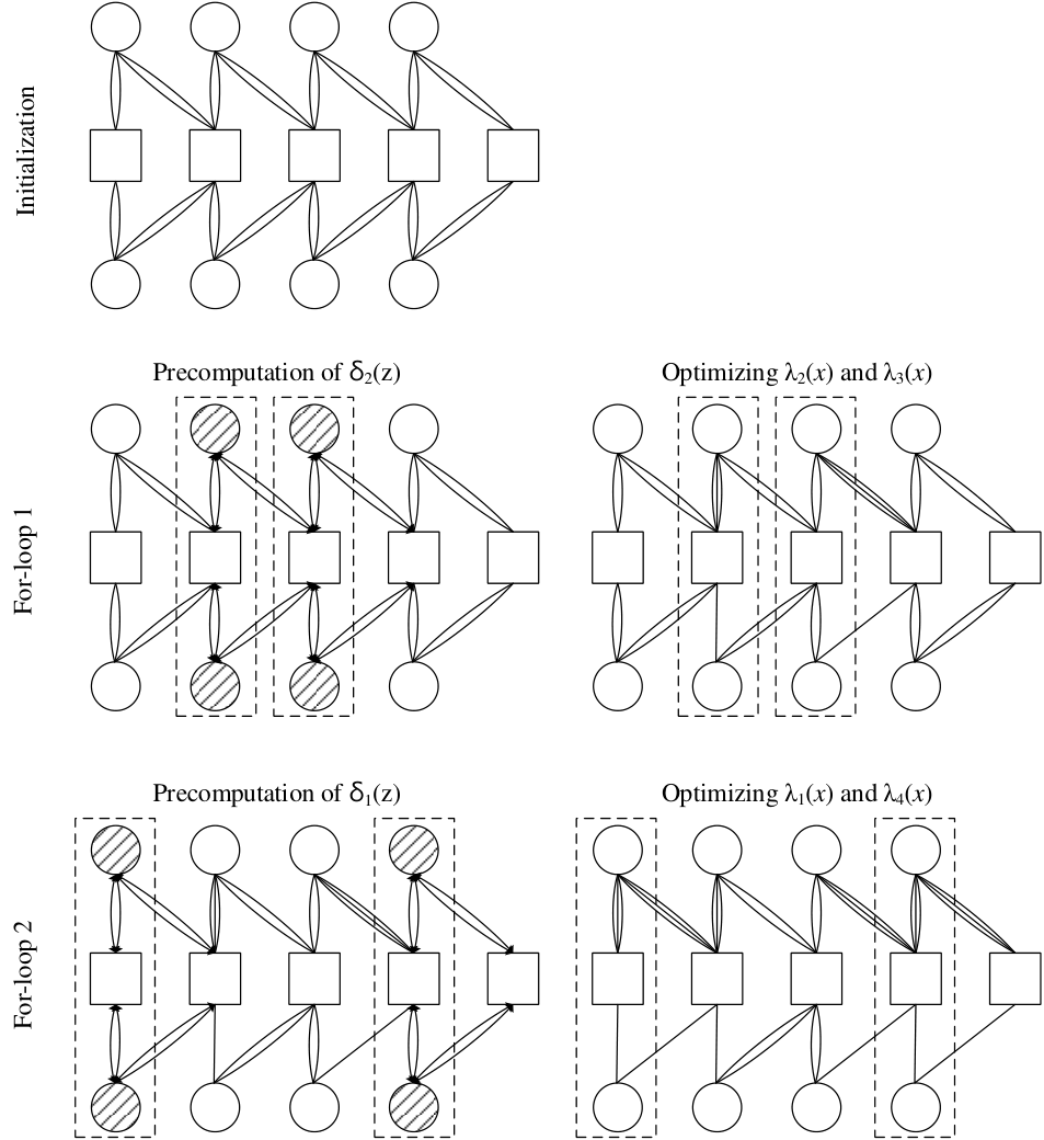
In Algorithm 2, the graph is initialized with the regular SC-LDPC ensemble. Then, the degree distribution $\lambda_{u}(x)$ is designed starting from $u=L/2\in\mathbb{N}$ to maximize the design rate and $\lambda_{L-u+1}(x)$ is also determined by the designed degree distribution because of the symmetric code structure. To design $\lambda_{L/2}(x)$, the value $\delta_{L/2}(z)$ is pre-calculated; this is used to design $\lambda_{L/2}(x)$ to maximize the design rate. The degree distribution for the next position $\lambda_{L/2-1}(x)$ is designed in the same manner after designing $\lambda_{L/2}(x)$. This local design is conducted until the number of iterations for the algorithm reaches $I_{\max}$ or $\lambda_{u}(x)$ does not change with $\rm{Iter}$. For the other algorithms to be introduced, we apply the same design procedure, in which the local design of the degree distributions is conducted for each pair of positions one at a time, as in Fig. 2.

For the input values $l=4,r=8,L=10,w=3,l_{\min}=3,l_{\max}=10,Q=1000$, and $I_{max}=10$, the design rate is increased from $0.4$ to $0.4360$ by Algorithm 2. Likewise, the design rate is increased from $0.45$ to $0.4670$ by Algorithm 2 for $L=20$. Fig. 3 shows the average variable node degree $1/{\int_{0}^{1}\lambda_{u}(x)dx}$ of each position for the SC-LDPC ensemble obtained by Algorithm 2 for $L=10$ and $20$. It shows that the degree distributions of the center positions $5,6$ for $L=10$ and $10,11$ for $L=20$ are properly designed to increase the design rate by minimizing the corresponding average variable node degrees. However, the variable node degrees of the positions far from the center positions remain nearly identical to the initial degree $l=4$. Thus, the fraction of the number of positions to be improved by Algorithm 2 becomes smaller as $L$ becomes larger. To achieve an improvement in all positions for large $L$, a different objective function for the LP problem is required instead of maximizing the design rate.

Another objective function described in Algorithm 3 is minimizing the number of required iterations. Consider a non-increasing iterative function $f(x)$. Given an initial value $a$, the iterative process is represented by $x^{(0)}=a$ and $x^{(\ell)}=f(x^{(\ell-1)})$. The number of required iterations $I(b)$ for the target value $b$, $b<a$, is defined as the minimum $\ell$ such that $x^{(\ell)}\leq b$. In [22], the number of required iterations $I(b)$ is approximated as

where $x_{0}=b,x_{n}=a,x_{i}=b+i\frac{a-b}{n}$, and $\Delta x_{i}=\frac{x_{i+1}-x_{i-1}}{2}$.

In the case of the one-dimensional DE $z^{(\ell+1)}=\epsilon\lambda_{u}(\delta_{u}(z^{(\ell)}))$ of the SC-LDPC ensemble, the iterative function is given as $f(x)=\epsilon\lambda_{u}(\delta_{u}(x))$. Thus, the number of required iterations from the initial value $z_{Q}=\epsilon$ to the target value $z_{1}=\epsilon/Q$ is approximated as

where $\Delta z_{q}=1/Q$. Thus, the design method that minimizes the number of iterations can be summarized as Algorithm 3, where the objective function is to minimize the equation (3). In Algorithm 3, there is the additional constraint ${1}/{\int_{0}^{1}\lambda^{*}(x)dx}=l$, which implies that the average variable node degree should be equal to the variable node degree $l$ of the initial regular SC-LDPC ensemble to maintain the design rate. As an example, some part of coefficients of $\lambda_{u}(x)$ obtained by Algorithm 3 with $l=4,r=8,L=20,w=3,l_{\min}=3,l_{\max}=10,Q=1000$, and $I_{max}=10$ are shown in Table II. Note that, to maintain the advantages of the regular SC-LDPC codes whose minimum variable node degree is larger than $2$ [26], we generally initialize the algorithm from the regular SC-LDPC ensemble with $l=4$ and the minimum degree constraint as $l_{\min}=3$. Instead, Algorithm 3 is not initialized from the regular SC-LDPC ensemble with $l=3$ because a non-zero fraction of degree-two variable nodes is unavoidably required to introduce a fraction of variable nodes with degree larger than $3$.

In order to investigate the change of the overall number of required iterations in the DE equations (2) at each local design, the evolution of the average convergence speed is shown in Fig. 4 as the for-loop in Algorithm 3 proceeds. It shows that the average convergence speed increases steadily as the local design of each position proceeds. In addition, we note an increase in the BP threshold at for-loop 6, where the BP threshold corresponds to the erasure probability that the average convergence speed becomes zero.

To observe the change in the SC-LDPC ensemble according to the local design of Algorithms 2 and 3 graphically, the expected graph evolution can be used. With the differential equations in Section II-C, Fig. 5 shows the evolutions of ${r}_{1}(\tau)$ at $\epsilon=0.48$ for the SC-LDPC ensembles obtained by the algorithms as the for-loop in the algorithms proceeds. The evolution of $r_{1}(\tau)$ at the initialization corresponds to $r_{1}(\tau)$ for the regular SC-LDPC ensemble that is analyzed in [25]. According to the analysis in [25], $r_{1}(\tau)$ remains constant at the local minimum for a certain interval of $\tau$, referred to as the critical phase. On the basis of the critical phase, the evolution of $r_{1}(\tau)$ is divided into three phases: The initial phase, the critical phase, and the third phase. Most of the variable nodes located in the boundary positions have already been recovered in the initial phase. Then, in the critical phase, two decoding waves emerge and travel along the inner positions while recovering the variable nodes through which the decoding waves pass. If the local performance of each position is defined as the number of degree-one check nodes when the decoding waves pass through the position, the steady value of $r_{1}(\tau)$ in the critical phase implies that the local performances of the inner positions are all the same. Moreover, it can be said that the BP threshold of the SC-LDPC ensemble is determined by the local performance of the inner positions. Finally, in the third phase, the decoding waves meet around the center and the variable nodes located at the center positions are recovered, which corresponds to the increase in the $r_{1}(\tau)$ value.

Fig. 5(a) shows the evolution of $r_{1}(\tau)$ as the for-loop in Algorithm 2 proceeds. After performing for-loop 2 in Algorithm 2, the degree distributions of the center positions from $9$ to $12$ are locally designed to decrease their average variable node degree. However, the value of $r_{1}(\tau)$ is decreased in the third phase at the expense of lowering the average variable node degrees of the center positions as in Fig. 5(a). In addition, it is observed that the minimum value of $r_{1}(\tau)$ in the third phase is nearly identical to the value of $r_{1}(\tau)$ in the critical phase due to the constraint in Algorithm 2 that the BP threshold should be maintained. If the minimum value of $r_{1}(\tau)$ in the third phase becomes smaller than the value of the critical phase, the BP threshold will be degraded. In other words, because the value of $r_{1}(\tau)$ in the third phase is larger than the critical phase value for the initial regular SC-LDPC ensemble, there is a room for improvement in the design rate for the center positions. However, an improvement in the design rate of the inner positions cannot be achieved while maintaining the BP threshold. Accordingly, the average variable node degree of the positions except the center positions does not change, as indicated in Fig. 3, and the evolution of $r_{1}(\tau)$ is unchanged from for-loops $2$ to $10$.

Compared to Algorithm 2, Fig. 5(b) shows the evolution of $r_{1}(\tau)$ as the for-loop in Algorithm 3 proceeds. After for-loop 2, where the local design has been performed from center positions $9$–$12$, $r_{1}(\tau)$ in the right part of the critical phase increases. This means that the local design improves the local performance of the center positions and accordingly the length of the critical phase is shortened and the overall number of required iterations is decreased. Likewise, from for-loops 2 to 4, the length of the critical phase is steadily shortened. After for-loop 6, the critical phase observed in the initial regular SC-LDPC ensemble disappears and only a single local minimum point remains. The local minimum value is greater than the value of $r_{1}(\tau)$ in the critical phase, which means that the BP threshold is increased. Further, in for-loop 8, the critical phase observed in the initialization completely disappears, which implies that the BP threshold is increased significantly. In other words, the BP threshold is increased in for-loop 6 because the local performances of positions $7$–$14$ have already been improved. Conversely, the BP threshold does not increase up to for-loop $4$ because the local performances of positions $1$–$6$ and $15$–$20$, which are not yet designed at this point, become a bottleneck despite the fact that the local performances of positions $7$–$14$ are improved by the local design. On the other hand, the BP threshold is increased when the bottleneck positions $5$ and $16$ are designed in for-loop $6$. In summary, the BP threshold can be increased if the degree distributions of all positions are properly designed by Algorithm 3. In Table III, the BP thresholds of the regular SC-LDPC ensemble and the SC-LDPC ensembles obtained by Algorithm 3 are shown.

It is important to remark that the degree distributions obtained by Algorithm 3 are not the global optimum that minimizes the overall number of required iterations in the DE equations (2) because of the two facts. First, the local design is performed instead of the global design. Second, the one-dimensional DE assumes different decoding scheduling from the conventional parallel scheduling as mentioned in Section III-A. Therefore, minimizing the number of required iterations in the one-dimensional DE equation does not guarantee minimization of the overall number of required iterations in parallel scheduling. However, we numerically observe that these two kinds of numbers of required iterations are generally proportional. Fig. 6 shows the correlation between the numbers of required iterations in the one-dimensional DE equation $z^{(\ell+1)}=\epsilon\lambda_{u}(\delta_{u}(z^{(\ell)}))$ and in DE equations (2) at for-loops 6 and 8 in Algorithm 3. Each point in Fig. 6 is the numbers of required iterations measured at $\epsilon=\epsilon^{\rm BP}-0.01$ for a randomly generated degree distribution. According to Fig. 6, it can be seen that both numbers of required iterations are generally proportional and thus the objective function of Algorithm 3 is proper for reducing the overall number of required iterations.

References

- [1] S. Kudekar, T. J. Richardson, and R. L. Urbanke, “Spatially coupled ensembles universally achieve capacity under belief propagation,” IEEE Trans. Inf. Theory, vol. 59, no. 12, pp. 7761–7813, Dec. 2013.
- [2] M. Lentmaier, A. Sridharan, D. J. Costello, Jr., and K. Sh. Zigangirov, “Iterative decoding threshold analysis for LDPC convolutional codes,” IEEE Trans. Inf. Theory, vol. 56, no. 10, pp. 5274–5289, Oct. 2010.
- [3] S. Kudekar, T. J. Richardson, and R. L. Urbanke, “Threshold saturation via spatial coupling: why convolutional LDPC ensembles perform so well over the BEC,” IEEE Trans. Inf. Theory, vol. 57, no. 2, pp. 803–834, Feb. 2011.
- [4] S. Kudekar, C. Measson, T. J. Richardson, and R. L. Urbanke, “Threshold saturation on BMS channels via spatial coupling,” in Proc. Int. Symp. Turbo Codes Iterative Inf. Process. (ISTC), Brest, France, Sep. 2010, pp. 309–313.
- [5] A. Yedla, Y.-Y. Jian, P. S. Nguyen, and H. D. Pfister, “A simple proof of threshold saturation for coupled scalar recursions,” in Proc. 7th Int. Symp. Turbo Codes Iterative Inf. Process. (ISTC), Gothenburg, Sweden, Aug. 2012, pp. 51–55.
- [6] ——, “A simple proof of Maxwell saturation for coupled scalar recursions,” IEEE Trans. Inf. Theory, vol. 60, no.11, pp. 6943–6965, Nov. 2014.
- [7] J. Thorpe, “Low-density parity-check (LDPC) codes constructed from protographs,” Jet Propulsion Lab., Pasadena, CA, USA, INP Progress Report 42–154, 2003.
- [8] D. Divsalar, H. Jin, and R. McEliece, “Coding theorems for turbo-like codes,” in Proc. 36th Allerton Conf. Commun. Control Comput., Monticello, IL, USA, 1998, pp. 201–210.
- [9] D. Divsalar, S. Dolinar, C. Jones, and K. Andrews, “Capacity approaching protograph codes,” IEEE J. Sel. Areas Commun., vol. 27, no. 6, pp. 876–888, Aug. 2009.
- [10] D. J. C. MacKay, “Good error-correcting codes based on very sparse matrices,” IEEE Trans. Inf. Theory, vol. 45, no. 2, pp. 399–431, Mar. 1999.
- [11] D. G. M. Mitchell, M. Lentmaier, and D. J. Costello, Jr., “New Families of LDPC block codes formed by terminating irregular protograph-based LDPC convolutional codes,” in Proc. IEEE Int. Symp. Inf. Theory (ISIT), Austin, Texas, USA, June 2010, pp. 824–828.
- [12] D. G. M. Mitchell, M. Lentmaier, and D. J. Costello, Jr., “Spatially coupled LDPC codes constructed from protographs,” IEEE Trans. Inf. Theory, vol. 61, no. 9, pp. 4866–4889, Sep. 2015.
- [13] K. Kasai and K. Sakaniwa, “Spatially-coupled MacKay-Neal codes and Hsu-Anastasopoulos codes,” in Proc. IEEE Int. Symp. Inf. Theory (ISIT), St. Petersburg, Russia, 2011, pp. 747–751.
- [14] N. Obata, Y.-Y. Jian, K. Kasai, and H. D. Pfister, “Spatially-coupled multi-edge type LDPC codes with bounded degrees that achieve capacity on the BEC under BP decoding,” in Proc. IEEE Int. Symp. Inf. Theory (ISIT), Istanbul, Turkey, 2013, pp. 2433–2437.
- [15] M. Stinner and P. M. Olmos, “On the waterfall performance of finite-length SC-LDPC codes constructed from protographs,” IEEE J. Sel. Areas Commun., vol. 34, no. 2, pp. 345–361, Feb. 2016.
- [16] S. Johnson and G. Lechner, “Spatially coupled repeat-accumulate codes,” IEEE Commun. Lett., vol. 17, no. 2, pp. 373–376, Feb. 2013.
- [17] W. Nitzold, G. P. Fettweis, and M. Lentmaier, “Spatially-coupled nearly regular LDPC code ensembles for rate-flexible code design,” in Proc. IEEE ICC, Sydney, NSW, Australia, Jun. 2014, pp. 2027–2032.
- [18] V. Aref, L. Schmalen, and S. ten Brink, “On the convergence speed of spatially coupled LDPC ensembles,” in Proc. 51st Annu. Allerton Conf. Commun., Control, Comput. (Allerton), Monticello, IL, USA, Oct. 2013, pp. 342–349.
- [19] L. Schmalen, V. Aref, J. Cho, D. Suikat, D. Rosener, and A. Leven, ”Spatially coupled soft-decision error correction for future lightwave systems,” J. Lightwave Technology, vol. 33, No. 5, pp. 1109–1116, Mar. 2015.
- [20] Y. Koganei, M. Yofune, C. Li, T. Hoshida, and Y. Amezawa “SC-LDPC code with nonuniform degree distribution optimized by using genetic algorithm,” IEEE Commun. Lett, vol. 20, no. 5, pp. 874–877, May 2016.
- [21] T. J. Richardson and R. Urbanke, Modern Coding Theory. Cambridge, U.K.: Cambridege Univ. Press, 2008.
- [22] V. Jamali, Y. Karimian, J. Huber, and M. A. Attari, “On the design of fast convergent LDPC codes for the BEC: An optimization approach,” IEEE Trans. Commun., vol. 63, no. 2, pp. 351–363, Feb, 2015.
- [23] M. R. Sanatkar and H. D. Pfister, “Increasing the rate of spatially-coupled codes via optimized irregular termination,” in Proc. Int. Symp. Turbo Codes Iterative Inf. Process. (ISTC), Sep. 2016, pp. 31–35.
- [24] B. Smith, M. Ardakani, W. Yu, and F. R. Kschischang, “Design of irregular LDPC codes with optimized performance-complexity tradeoff,” IEEE Trans. Commun., vol. 58, no. 2, pp. 489–499, Feb. 2010.
- [25] P. M. Olmos and R. Urbanke, “A scaling law to predict the finite-length performance of spatially coupled LDPC codes,” IEEE Trans. Inf. Theory, vol. 61, no. 6, pp. 3164–3184, Jun. 2015.
- [26] D. J. Costello, Jr., L. Dolecek, T. E. Fuja, J. Kliewer, D. G. M. Mitchell, and R. Smarandache, “Spatially coupled sparse codes on graphs: Theory and practice,” IEEE Commun. Mag., vol. 52, no. 7, pp. 168–176, Jul. 2014.
- [27] X.-Y. Hu, E. Eleftheriou, and D. Arnold, “Regular and irregular progressive edge-growth Tanner graphs,” IEEE Trans. Inf. Theory, vol. 51, no. 1, pp. 386–398, Jan. 2005.