Continuous Level Monte Carlo and Sample-Adaptive Model Hierarchies

Suppose one is interested in estimating the expected value $\mathbb{E}[\mathcal{Q}]$ of some (inaccessible) quantity of interest $\mathcal{Q}$, for simplicity assumed to be scalar. In uncertainty quantification (UQ), $\mathcal{Q}$ is typically a functional of the solution of some random partial differential equation (PDE), where the randomness can lie anywhere, e.g. within the coefficients, the source, the boundary conditions or the shape of the domain.

In general, the solution of a PDE can not be calculated exactly and it has to be approximated numerically, up to some desirable resolution level $L$. Let us call $Q_{L}$ such an approximation and assume that $Q_{L}\to\mathcal{Q}$ almost surely (a.s.) for $L\to+\infty$. Then, for any desired tolerance $\varepsilon>0$, there exists a fine enough resolution $L$, such that $|\mathbb{E}[\mathcal{Q}-Q_{L}]|\leq\varepsilon$, and we can focus on finding good algorithms to estimate $\mathbb{E}[Q_{L}]$ to the same accuracy. There are two main issues here.

1. 1.

   If the underlying probability distribution is continuous and high-dimensional, which is common in UQ applications, it can be extremely expensive to approximate the expected value with standard quadrature methods.

2. 2.

   If the resolution $L$ required to compute the PDE solution with sufficient accuracy is high, then computing just one sample of $Q_{L}$ will be expensive and the number of samples that can be computed on level $L$ in a reasonable time is limited.

A standard remedy for Issue 1 is the use of Monte Carlo (MC) methods [19]. Indeed, the rate of converge of MC estimators is independent of the dimension of the integral and it is extremely easy to implement: given $N$ independent samples $\big(Q_{L}^{(k)}\big)_{k=1}^{N}$ of $Q_{L}$, distributed according to the underlying probability distribution, the expected value can be estimated as

$$\mathbb{E}[Q_{L}]\approx\frac{1}{N}\sum_{k=1}^{N}Q_{L}^{(k)}.$$

(1)

Whilst the right-hand-side in (1) is an unbiased estimator of $\mathbb{E}[Q_{L}]$, unfortunately it converges very slow, especially when $L$ is large, since $\mathcal{O}(\varepsilon^{-2})$ samples are required to reduce the sampling error to a given accuracy $\varepsilon$, i.e. $|\mathbb{E}[\mathcal{Q}-Q_{L}]|\leq\varepsilon$. As every sample requires an expensive PDE solve, the computational cost quickly becomes infeasible for small $\varepsilon$.

An acceleration technique suggested for (1) is the multilevel Monte Carlo (MLMC) method [13, 9]. It exploits a hierarchy of approximations $Q_{0},Q_{1},\dots,Q_{L}$ of $\mathcal{Q}$ at different resolutions, starting with a coarse and cheap approximation $Q_{0}$, and going up to the fine and expensive approximation $Q_{L}$. In contrast to the standard MC estimator in (1), which directly estimates $\mathbb{E}[Q_{L}]$ by sampling $Q_{L}$, MLMC combines samples from the sequence of approximations $(Q_{\ell})_{\ell=0}^{L}$ to produce an overall cheaper estimator. To this purpose, the approximations are combined into the telescoping sum

$$\mathbb{E}[Q_{L}-Q_{0}]=\sum_{\ell=1}^{L}\mathbb{E}[Q_{\ell}-Q_{\ell-1}],$$

(2)

and then each term in the sum on the right-hand-side is estimated with Monte Carlo:

$$\mathbb{E}[Q_{\ell}-Q_{\ell-1}]\approx\frac{1}{N_{\ell}}\sum_{k=1}^{N_{\ell}}\left(Q_{\ell}^{(k)}-Q_{\ell-1}^{(k)}\right).$$

(3)

To obtain an estimator for $\mathbb{E}[Q_{L}]$ it suffices to add a Monte Carlo estimator for $\mathbb{E}[Q_{0}]$.

Crucially, the consecutive approximations $Q_{\ell-1}^{(k)}$ and $Q_{\ell}^{(k)}$ in the difference $Q_{\ell}^{(k)}-Q_{\ell-1}^{(k)}$ come from the same sample $k$. This means that they are strongly positively correlated, and the variance of the difference is heavily reduced:

$$\mathbb{V}[Q_{\ell}-Q_{\ell-1}]=\mathbb{V}[Q_{\ell-1}]+\mathbb{V}[Q_{\ell}]-2\textnormal{Cov}(Q_{\ell-1},Q_{\ell})\ll\mathbb{V}[Q_{\ell-1}]+\mathbb{V}[Q_{\ell}].$$

(4)

As $Q_{\ell}\to\mathcal{Q}$ a.s. for $\ell\to+\infty$, we also have $Q_{\ell}-Q_{\ell-1}\to 0$, so that the covariance, and in turn the variance reduction, increases as $\ell\to+\infty$. As a consequence, the required number of samples $N_{\ell}$ at level $\ell$ can be chosen to decrease monotonically with increasing $\ell$, so that only very few expensive samples on level $L$ are needed. The majority of samples and therefore the computational cost will be shifted to the coarser levels.

This reduction in computational complexity can be quantified rigorously, at least asymptotically as the tolerance $\varepsilon\to 0$. The complexity theorems in [9, 4] show that the overall computational cost for the MLMC algorithm can be up to a factor $\mathcal{O}(\varepsilon^{2})$ smaller than the cost of the MC estimator in (1). We will return to this and give more details in Section 2.4.

In this section, we introduce the continuous level Monte Carlo (CLMC) idea. As we have seen above, MLMC exploits a discrete sequence of approximations $(Q_{\ell})_{\ell=0}^{L}$ of $\mathcal{Q}$. We now extend this to a continuous family of approximations $(Q(\ell))_{\ell\geq 0}$ of $\mathcal{Q}$. In other words, $(Q(\ell))_{\ell\geq 0}$ is a stochastic process of approximations over the continuous level of resolution $\ell$.

Let $L$ be assumed to be a random variable with finite expectation denoting the (random) finest level of resolution, independent from the stochastic process $(Q(\ell))_{\ell\geq 0}$. Also, let $L_{\max}\in[0,\infty]$ be a deterministic constant that we introduce for reasons that will become clearer later. We can write down the following formula:

$$\mathbb{E}[Q(L\wedge L_{\max})-Q(0)]=\mathbb{E}\left[\int_{0}^{L\wedge L_{\max}}\frac{\text{d}Q(\ell)}{\text{d}\ell}\,\text{d}\ell\right]\,.$$

(5)

For the formula in (5) to be well-posed, we need to assume that $Q\in W^{1,1}(0,L_{\max})$ as a function of $\ell$, where $W^{1,1}(0,L_{\max})$ is a Sobolev space containing functions over $\ell\in(0,L_{\max})$ such that the functions and their weak first derivatives have finite $L^{1}$ norm. Note that for simplicity we are choosing 0 as coarsest level, but this can of course be generalised.

If we assume $L$ to be a deterministic variable, the expectation in (5) can be pulled inside the integral and the derivative, so that equation (5) reduces to the Fundamental Theorem of Calculus, which guarantees the identity. However, more generally, equation (5) can be recovered as a particular case of Dynkin’s Formula [17], where $L$ is interpreted as a finite stopping time.

Let us assume $L$ to be a random variable independent of the whole stochastic process $(Q(\ell))_{\ell\geq 0}$. We can then define the continuous level Monte Carlo (CLMC) estimator

$$\widehat{Q}^{\text{CLMC}}_{L_{\max}}:=\frac{1}{N}\sum_{k=1}^{N}\int_{0}^{L_{\max}}\frac{1}{\mathbb{P}(L\geq\ell)}\left(\frac{\text{d}Q}{\text{d}\ell}\right)^{(k)}(\ell)\,\mathbbm{1}_{[0,L^{(k)}]}(\ell)\,\text{d}\ell,$$

(6)

where the superscript $(k)$ denotes the $k$-th realisation of the respective random variable and $N$ is the total number of samples. For simplicity of presentation, the estimator $\widehat{Q}^{\text{CLMC}}_{L_{\max}}$ is defined as an estimator for $\mathbb{E}[Q(L_{\max})-Q(0)]$, as we see in Proposition 2.1. As in standard MLMC, it suffices to add an unbiased estimator for $\mathbb{E}[Q(0)]$ to obtain an estimator for $\mathbb{E}[Q(L_{\max})]$.

A reader familiar with the MLMC literature might be puzzled by the estimator in (6), where we use the same number of samples $N$ for each level $\ell$. However, note that, for each sample $k$, the integrand in (6) will only be non-zero up to the random realisation $L^{(k)}$ of $L$, and therefore in practice we do not need to evaluate $Q(\ell)$ beyond level $L^{(k)}$.

We are now ready to show that the CLMC estimator is unbiased.

In particular, this implies the following important corollary.

Corollary 2.2 shows that there is a version of the estimator (6) that is unbiased with respect to the expectation of the difference of the real quantity of interest $\mathcal{Q}$ and $Q(0)$, and one can see the connection with the unbiased MLMC estimator introduced in [18].

In the next subsection, we will prove a complexity theorem for the CLMC estimator (6). We will pick $L$ to be distributed as an exponential random variable to facilitate calculations and mimic the exponential decay in the assumptions on the convergence of the quantity of interest. Also, we will provide sufficient and necessary conditions for the Theorem to hold in the case $L_{\max}=+\infty$, i.e. when the CLMC estimator is unbiased with respect to $\mathcal{Q}-Q(0)$. A practical algorithm will then be described in Section 3.

The fundamental theoretical result about the MLMC method is the complexity theorem, firstly proved in [9] and generalised in [4]. In this section, we state an analogous complexity theorem for the CLMC estimator (6). A full proof is given in Appendix A.

First, let us define the mean-squared-error (MSE) of the CLMC estimator $\widehat{Q}^{\text{CLMC}}_{L_{\max}}$ in (6) by

$$\text{MSE}:=\mathbb{E}\left[\big(\widehat{Q}^{\text{CLMC}}_{L_{\max}}-\mathbb{E}[\mathcal{Q}-Q(0)]\big)^{2}\right]$$

(7)

and denote by $\mathcal{C}^{\textnormal{CLMC}}_{L_{\max}}$ its expected computational cost. Then, we have the following result.

Note that the predicted computational cost in Theorem 2.3 is the same as in MLMC (asymptotically).

Corollary 2.4 provides sufficient and necessary conditions for the CLMC estimator with $L_{\max}=+\infty$ (which is unbiased with respect to $\mathcal{Q}-Q(0)$) to have a finite expected complexity cost. Intuitively, since $L_{\max}=+\infty$, the finest level at which computations are needed is $\max_{k=1}^{N}L^{(k)}$, which tends to infinity as $N$ grows. Therefore, the estimator (6) will have finite expected cost only if the actual variance reduction rate is bigger than the actual cost growth rate. The rates $\beta$ and $\gamma$ in Theorem 2.3 are only upper bounds. By analogy, we believe this constraint also applies to the unbiased estimator introduced by Rhee & Glynn [18]. However, the paper [18] is mainly concerned with timestepping methods for SDEs, where the condition $\gamma<\beta$ is usually satisfied.

Note that, if $L_{\max}=+\infty$, even in the case $\beta>\gamma$, there is a non-zero probability that the finest level $L^{(k)}$ for some sample $(k)$ is drawn larger than the maximal refinement achievable on the particular machine that is used, but we can exactly quantify the probability for this to happen. Indeed, if $\bar{L}$ is the maximum refinement level achievable by the machine, the probability that at least one sample is greater or equal than $\bar{L}$ is given by

$$N\mathbb{P}(L\geq\bar{L})=N\exp(-r\bar{L}).$$

We will see that for problems of interests this probability is very small. In the rare event that $L^{(k)}>\bar{L}$ for some sample $k$, one could simply approximate $Q^{(k)}(\ell)=Q^{(k)}(\bar{L})$ for $\ell\in[\bar{L},L^{(k)}]$. If $\bar{L}$ is sufficiently large, this would introduce a negligible bias error to any practical values of $\varepsilon$.

Let us assume that we have estimates of the parameters $\alpha,\beta,\gamma$ in Theorem 2.3. In practice, these can be obtained (on the fly) from sample averages and sample variances of $Q(\ell)$ and $\text{d}Q(\ell)/\text{d}\ell$, as in standard MLMC. Then, given a desired tolerance $\varepsilon>0$, Theorem 2.3 provides suitable choices for the number of samples $N$ and for the rate $r$ of the exponential distribution of $L$ to achieve the optimal complexity in (8).

For any sample $k$, suppose that $(Q_{j}^{(k)})_{j\geq 1}$ denotes a countable sequence of approximations of $Q^{(k)}$ at levels $(\ell_{j}^{(k)})_{j\geq 1}$. Then, to define a continuous family $Q^{(k)}(\ell)$ of $Q^{(k)}$, we use linear interpolation such that

$$\left(\frac{\text{d}Q}{\text{d}\ell}\right)^{(k)}(\ell):=\frac{Q_{j}^{(k)}-Q_{j-1}^{(k)}}{\ell^{(k)}_{j}-\ell^{(k)}_{j-1}}\quad\quad\textnormal{for }\ell\in(\ell_{j-1}^{(k)},\ell_{j}^{(k)})\,.$$

Also, for each sample $k$, let us define the index $J^{(k)}$ corresponding to the first value of $\ell_{j}^{(k)}$ that is bigger than $L^{(k)}\wedge L_{\max}$, that is

$$J^{(k)}:=\min\{j\geq 1:\ \ell_{j}^{(k)}-(L^{(k)}\wedge L_{\max})\geq 0\}.$$

Hence, we can write down the CLMC estimator (6) as

	$\displaystyle\widehat{Q}^{\textnormal{CLMC}}_{L_{\max}}$	$\displaystyle=\frac{1}{N}\sum_{k=1}^{N}\int_{0}^{L^{(k)}\wedge L_{\max}}\frac{1}{P(L\geq\ell)}\left(\frac{\text{d}Q}{\text{d}\ell}\right)^{(k)}(\ell)\,\text{d}\ell$
		$\displaystyle=\frac{1}{N}\sum_{k=1}^{N}\sum_{j=1}^{J^{(k)}}w_{j}^{(k)}\left(Q_{j}^{(k)}-Q_{j-1}^{(k)}\right)\,,$		(9)

where we define

$$\tilde{\ell}_{j}^{(k)}:=\ell_{j}^{(k)}\wedge(L^{(k)}\wedge L_{\max})\,,$$

(10)

and the integrals in the weights $w_{j}^{(k)}$ can be computed explicitly as

$$w_{j}^{(k)}:=\frac{1}{\ell^{(k)}_{j}-\ell^{(k)}_{j-1}}\int_{\ell_{j-1}^{(k)}}^{\tilde{\ell}_{j}^{(k)}}\frac{1}{P(L\geq\ell)}\,\text{d}\ell=\frac{\exp\big(r\tilde{\ell}_{j}^{(k)}\big)-\exp\big(r\ell_{j-1}^{(k)}\big)}{r\big(\ell^{(k)}_{j}-\ell^{(k)}_{j-1}\big)}\,,$$

(11)

for all $j=1,\ldots,J^{(k)}$ . Algorithm 1 provides the key instructions to implement the CLMC estimator in (9).
Algorithm 1 CLMC algorithm – Key steps Input : $\varepsilon$: tolerance; $r$: exponential rate; $N$: total number of samples; $L_{\max}$: maximum reachable level - potentially infinite if $\gamma<\beta$. Output : $\widehat{Q}^{\textnormal{CLMC}}_{L_{\max}}$: CLMC estimator. 1:  Initialise $\hat{Q}\leftarrow 0$; 2:  for $k=1,2,\dots,N$ do 3:   Sample $L^{(k)}\sim\textnormal{Exponential}(r)$; 4:   Evaluate and store quantity of interests $Q\leftarrow(Q_{j}^{(k)})_{j=1}^{J^{(k)}}$ at levels $\ell\leftarrow(\ell_{j}^{(k)})_{j=1}^{J^{(k)}}$; 5:   Calculate array $w$ of weights in (11); 6:   Update $\widehat{Q}^{\textnormal{CLMC}}_{L_{\max}}\leftarrow\widehat{Q}^{\textnormal{CLMC}}_{L_{\max}}+w^{T}*\textnormal{diff}(Q)$, where $\textnormal{diff}(Q)$ is the array of the differences between consecutive elements of $Q$; 7:  end for 8:  Set $\widehat{Q}^{\textnormal{CLMC}}_{L_{\max}}\leftarrow\widehat{Q}^{\textnormal{CLMC}}_{L_{\max}}/N$.

Note that it is easy to work out an unbiased estimator for the variance of $\widehat{Q}^{\textnormal{CLMC}}_{L_{\max}}$ in (9), which is needed to estimate the total number of samples $N$. Let us define

$$Y^{(k)}:=\sum_{j=1}^{J^{(k)}}w_{j}^{(k)}\left(Q_{j}^{(k)}-Q_{j-1}^{(k)}\right)\,.$$

Then (9) simply reduces to a standard Monte Carlo estimator with i.i.d. samples $Y^{(k)}$ and we can estimate

$$\mathbb{V}\left[\widehat{Q}^{\textnormal{CLMC}}_{L_{\max}}\right]\approx\frac{1}{N(N-1)}\sum_{k=1}^{N}\left(\,\left(Y^{(k)}\right)^{2}-\left(\frac{1}{N}\sum_{i=1}^{N}Y^{(i)}\right)^{2}\,\right)\,.$$

It is interesting to see what happens in the case of uniform refinements, where all samples $Q^{(k)}$, for $k=1,\ldots,N$, are evaluated at the same deterministic points $\ell_{j}^{(k)}=\ell_{j}$, for $j\geq 1$, and then interpolated. Without loss of generality, we assume that $\ell_{j}=j$, as in standard MLMC.

In this case, the set of possible levels reduces to integers. Therefore, although a continuous probability distribution for $L$ is still a valid choice, it is more natural to pick a discrete distribution over the levels, where $\mathbb{P}(L\geq j)$ is constant over the interval $(j-1,j)$. In that case, the practical CLMC estimator in (9) reduces to

$$\widehat{Q}^{\textnormal{CLMC}}_{L_{\max}}=\frac{1}{N}\sum_{k=1}^{N}\sum_{j=1}^{J^{(k)}}\frac{1}{\mathbb{P}(L\geq j)}\left(Q_{j}^{(k)}-Q_{j-1}^{(k)}\right)\,.$$

A natural choice would be a geometric distribution on $L$.

To see the relationship with the standard MLMC estimator more clearly, let us define

$$N(\ell):=N\mathbb{P}(L\geq\ell)\,.$$

Then, $(N(\ell))_{\ell\geq 0}\subset[0,\infty)$ corresponds to a continuous density of samples, analogous to the sequence of sample sizes at discrete levels in MLMC. Moreover, the probability that $L$ is at least $\ell$ corresponds to the normalised density of samples that gets at least to level $\ell$. Therefore, by plugging this relation in the equation above, we get

$$\widehat{Q}^{\textnormal{CLMC}}_{L_{\max}}=\sum_{k=1}^{N}\sum_{j=1}^{J^{(k)}}\frac{1}{N(\ell)}\left(Q_{j}^{(k)}-Q_{j-1}^{(k)}\right)\,,$$

which exactly corresponds to the Rhee & Glynn estimator in [18].

We consider a toy-model describing steady state, single phase, incompressible flow in a permeable medium (e.g. rock), given by the linear, scalar elliptic partial differential equation

$$-\nabla\cdot k({\bf x})\nabla u({\bf x})=f({\bf x})\quad\forall{\bf x}\in D\subset\mathbb{R}^{d},$$

(15)

subject to suitable boundary conditions. Physically $u({\bf x})$ is the fluid pressure, $f({\bf x})$ the fluid source term and $k({\bf x})$ the scalar permeability field. In practical applications (e.g. in oil reservoir simulation), the permeability field $k({\bf x})$ or the source term $f({\bf x})$ are not known everywhere, therefore a typical approach is to model each as a random field. Let the sample space be denoted by $\Omega$, then the random permeability and source field $k({\bf x},\omega)$ and $f({\bf x},\omega)$ belong to $D\times\Omega$ with a certain distribution (inferred from data). Therefore the solution to (15), the unknown pressure field, is also a random field i.e. $u({\bf x},\omega)\in D\times\Omega$. For simplicity, we shall restrict ourselves to homogeneous Dirichlet conditions $u(\omega,\cdot)\equiv 0$ on the domain boundary $\partial D$.

For a fixed $\omega\in\Omega$ we can recast (15) as a standard variational problem, i.e. find $u({\bf x},\omega)\in V:=H^{1}_{0}(D)=\{v\in H^{1}(D):v=0\;\mbox{on}\;\partial D\}$, such that

$$\underbrace{\int_{D}k({\bf x},\omega)\nabla u\cdot\nabla v\;d{\bf x}}_{=:\;a(\omega;u,v)}\;=\;\underbrace{\int_{D}f({\bf x},\omega)v\;d{\bf x}}_{=:b(\omega;v)}\;\,,\qquad\forall v\in V\,.$$

(16)

Here, $D$ is assumed to be a bounded Lipschitz domain and $V=H^{1}_{0}(D)$ is the usual Sobolev space of weakly differentiable functions on $D$. Then, $a(\omega;\cdot,\cdot)$ is a symmetric, bounded and positive-definite bilinear form on $V\times V$, and as such defines an inner product and a norm on $V$,the so-called energy norm $\|u\|_{a}:=\sqrt{a(u,u)}$. If $f$ is sufficiently smooth, then the functional $b(\omega;\cdot)$ is bounded on $V$.

To approximate the pressure solution $u({\bf x},\omega)$, we construct a (sample-wise adapted) finite element (FE) space $V_{h}(\omega)\subset V$ of piecewise linear Lagrange polynomials on a grid $\mathcal{T}_{h}(\omega)$ that vanish on the boundary of $D$. The FE solution $u_{h}({\bf x},\omega)\in V_{h}(\omega)$ satisfies

$$a(\omega;u_{h},v_{h})=b(\omega;v_{h})\,,\qquad\forall v_{h}\in V_{h}(\omega),$$

(17)

resulting in a (large) linear system of equations of dimension $M_{h}(\omega):=\dim(V_{h}(\omega))$. From this, we are interested in approximating statistics (e.g. the expected value) of a quantity of interest $\mathcal{Q}$, defined to be (for simplicity) a linear functional of $u_{h}({\bf x},\omega)$.

As motivated at the beginning of this section, we are going to build our approximate solutions, sample-by-sample using adaptive finite element methods. But instead of using the number of refinement steps as the level parameter and applying MLMC, we will use a sample-wise error estimate as the level parameter and apply our new CLMC framework.

For any $\omega\in\Omega$, starting with an initial grid $\mathcal{T}^{(0)}(\omega)$, chosen to be the same for each sample, we use an $h$-adaptive refinement strategy to construct a sequence of grids $\mathcal{T}^{(k)}(\omega)$ for $k=0,\ldots,K$. In our case, the adaptive procedure is driven by a local, goal-orientated error indicator $e_{\tau}^{(k)}(\omega)$, for each $\tau\in\mathcal{T}^{(k)}(\omega)$. This gives the relative contribution from each element to the error in the quantity of interest $\mathcal{Q}(u(\omega))$, so that

$$|\mathcal{Q}(u(\omega))-\mathcal{Q}(u^{(k)}(\omega))|\leq e^{(k)}(\omega)=\left(\sum_{\tau\in\mathcal{T}^{(k)}(\omega)}e_{\tau}^{(k)}(\omega)\right)^{1/2}\,.$$

(18)

In addition to solving (17) (the so-called primal problem), goal-oriented error estimators typically also require an approximate FE solution $w_{h}(\omega,{\bf x})$ of the dual problem

$$a(\omega;v_{h},w_{h})=\mathcal{Q}(v_{h})\quad\forall v_{h}\in V_{h}.$$

(19)

There are many different choices of goal-oriented error estimators, see for example [11]. For one particular choice, described in detail in [11], the error estimator $e_{\tau}^{(k)}(\omega)$ in each element $\tau\in\mathcal{T}^{(k)}$ is computed by bounding the product of the energy norms of the errors in the primal and dual FE solutions $u_{h}(\omega,{\bf x})$ and $w_{h}(\omega,{\bf x})$ of (17) and (19), respectively. Up to a sample-dependent constant, these bounds are simply the sum of the element residuals and of the jumps/discontinuities in inter-element fluxes for each of the two problems. Full details can be found in [11], but we will also provide some more details in Appendix B.

The FE grid $\mathcal{T}^{(k+1)}(\omega)$ is generated by refining the $\theta^{(k)}$ percent of elements of $\mathcal{T}^{(k)}(\omega)$ that contribute most to the error in $\mathcal{Q}$ as defined by (18). This is typically followed by some additional refinements that ensure that the FE space $V^{(k+1)}(\omega)$ is conforming, i.e. that there are no hanging nodes in $\mathcal{T}^{(k+1)}(\omega)$. In our numerical experiments below, we increase $\theta^{(k)}$ as $k$ increases and use a so-called red/green refinement strategy that ensures conformity.

Finally, we now define our sample-wise continuous level at refinement step $k$ to be

$$\ell_{k}(\omega)=-\log\left(\frac{e^{(k)}(\omega)}{e^{(0)}(\omega)}\right)$$

(20)

The level gives a sample-wise measure of the error in $Q_{k}(\omega)$, the quantity of interest computed on $\mathcal{T}^{(k+1)}(\omega)$, relative to the error on the coarsest grid. We note that with this choice, computations on $\mathcal{T}^{(0)}$ are naturally providing values $Q_{0}(\omega)$ at level $\ell_{0}(\omega)=0$. However, the main reason for defining the error in this way is due to the explicit error estimator that are being used being only known up to an unknown constant (dependent on $\omega$).

All the numerical experiments are calculated using the high performance FE library DUNE [2] and its discretisation module dune-pdelab. Simulations are carried out on a computer consisting of four, 8-core Intel Xeon E5-4627v2 Ivybridge processors, each running at 1.2 GHz, giving a total of 32 available cores. The solutions for each sample are computed on a single processor and independent samples are equally distributed across all available cores. Individual solutions of the forward and dual problems are obtained using the sparse direct solver UMFPACK [5]. Each adaptive step uses the red/green refinement strategy, as implemented in dune-grid [1], refining $\theta^{(k)}$ percent of elements from $\mathcal{T}^{(k)}$ to $\mathcal{T}^{(k+1)}$.

In our numerical test, we consider $D:=[0,1]^{2}$. The coarse grid $\mathcal{T}^{(0)}$ for all samples is taken as a uniform $32\times 32$ triangular mesh on $D$. In our test we consider (15) with random permeability field $k$ and random source term $f$. The permeability field $k({\bf x},\omega)$ is characterised by a log-normal random field, where $\log k({\bf x},\omega)$ has a mean of zero and a two-point exponential covariance function

$$C({\bf x},{\bf y}):=\exp\left(-3\,\|{\bf x}-{\bf y}\|_{1}\right)\quad{\bf x},{\bf y}\in D,$$

(21)

with $\|\cdot\|_{p}$ denoting the $\ell_{p}$-norm in $\mathbb{R}^{2}$. The field is parameterised with a (truncated) Karhunen-Loève (KL) expansion

$$k({\bf x},\omega)=\exp\left(\sum_{i=1}^{R}\sqrt{\mu_{i}}\phi_{i}({\bf x})\xi_{i}\right).$$

(22)

where $\{\mu_{i}\}_{i\in\mathbb{N}}$ are the eigenvalues, $\{\phi_{i}({\bf x})\}_{i\in\mathbb{N}}$ the corresponding $L_{2}$-normalised eigenfunctions of the covariance operator with kernel function $C({\bf x},{\bf y})$ and $\xi_{i}\sim\mathcal{N}(0,1)$. For more details on how this expansion is constructed see for example [4]. In the calculations which follow we take $R=36$. For the random source term, we take

$$f({\bf x},\omega)=1000\,a\;\exp\left(-20\|{\bf x}-{\bf y}_{f}\|^{2}_{2}\right)$$

(23)

where $a$ and the components of ${\bf y}_{f}$ are all sampled from $\mathcal{U}(0,1)$.

As the quantity of interest, we consider the average pressure near ${\bf y}_{Q}:=[0.25,0.25]^{T}$, defined by the linear functional

$$\mathcal{Q}(u):=C_{1}\int_{D}\exp\left(-\frac{\|{\bf x}-{\bf y}_{Q}\|_{2}^{2}}{\lambda_{Q}}\right)u({\bf x},\omega)d{\bf x},$$

(24)

with $\lambda_{Q}=0.0005$ and $C_{1}=\left(\int_{D}\exp(-\|{\bf x}-{\bf y}_{Q}\|_{2}^{2}/\lambda_{Q})d{\bf x}\right)^{-1}\approx 0.00157$.

We now test our CLMC algorithm (Algorithm 1) by comparing uniform refinements and adaptive refinements with a variable $\theta^{(k)}$ (percentage of elements refined per step). In particular, we choose

$$\theta^{(k)}=\min(100\%,\delta^{k}\theta_{0})$$

(25)

as the percentage of elements refined in $\mathcal{T}^{(k)}$, with $\theta_{0}=1\%$ and $\delta=3$. We note that this choice is heuristic, motivated by a series of test runs. For the problem at hand, the idea of starting with small $\theta^{(0)}$ and increasing the percentage with the number of adaptive steps makes sense. Initially the error in $\mathcal{Q}$ is dominate by the fact that the grid is not well adapted to the particular random sample $\omega\in\Omega$. This includes the random field, the location of the localised source and the quantity of interest itself. Once the adaptive strategy has focused in on all those localised regions, the error in $\mathcal{Q}$ is governed by the global lack of singularity in the coefficient [3, 20] and thus distributed fairly uniformly across the whole domain. So from that point onwards, refining all elements uniformly leads to the most effective error reduction.

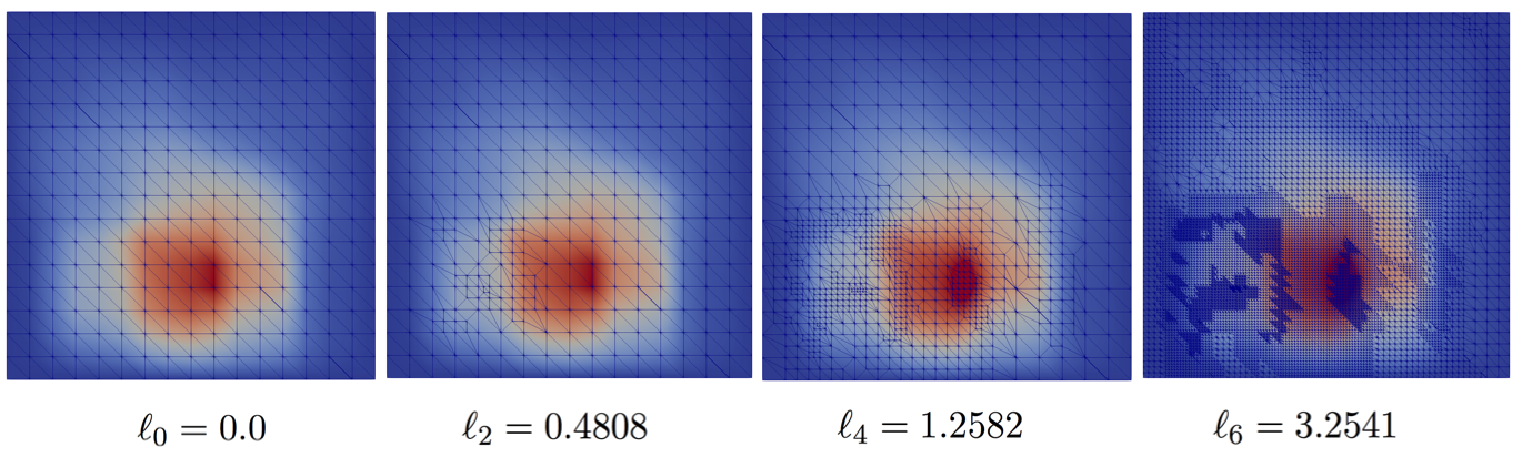
Before running a complete simulation we first consider a single sample $\omega\in\Omega$. Figure 1 shows the random permeability field $k({\bf x},\omega)$, pressure solution $u_{h}({\bf x},\omega)$, and the influence function $w_{h}({\bf x},\omega)$ (i.e. the solution of the dual problem (19)) for this sample after $6$ adaptive steps. Snapshots of the grids, built using the goal-oriented error estimator, are shown in Figure 2 at steps $0$, $2$, $4$ and $6$. Visually, we see that the adaptive scheme is working correctly, refining near ${\bf y}_{Q}=[0.25,0.25]^{T}$, the point around which the pressure is averaged in the functional $\mathcal{Q}$ in (24), whilst also adapting around the localised source. At the latter levels the refinement also starts to pick up local variations in the permeability field in regions that influence the pressure at the point of interest.

For the uniform and adaptive strategy, we first run an initial batch of $6400$ samples up to $L_{\max}=5$, in order to estimate the parameters $\beta$ and $\gamma$. In a real simulation, it would not be necessary to estimate these parameters accurately and so significantly fewer samples could be used. With uniform refinements, our estimates are $\beta_{u}=2.28$ and $\gamma_{u}=1.0$, whereas for adaptive refinements we get $\beta_{a}=2.22$ and $\gamma_{a}=0.78$. Note that, in both cases, $\beta>\gamma$, therefore by taking $L_{\max}=+\infty$ in the CLMC setting we obtain unbiased estimators with respect to $\mathbb{E}[\mathcal{Q}-Q(0)]$. In these initial runs we can already see the expected computational gains of adaptive grid refinement. We note that the rates $\beta$ for $\mathbb{V}[dQ/d\ell]$ are much the same in each case, whilst $\gamma$, the rate of growth of the expected cost per sample, is clearly smaller for the adaptive strategy. Figure 3 gives a plot of the continuous level $\ell$, representing the estimate of the relative finite element error, against the natural log of the cost for all samples, which shows the better rate for the adaptive scheme.

We then run the CLMC algorithm with a maximum of $N=10^{6}$ samples for each case. The exponential parameter rate $r$ is taken to be the same for each case, so that any computational gains can be attributed to the adaptive strategy, rather than a difference in $r$. The value is chosen so that $r=\frac{1}{2}(r_{u}+r_{a})=\frac{1}{4}(\beta_{u}+\gamma_{u}+\beta_{a}+\gamma_{a})=1.57$, and we consider the unbiased estimator with $L_{\max}=+\infty$.

References

- [1] P. Bastian, M. Blatt, A. Dedner, C. Engwer, R. Klöfkorn, M. Ohlberger and O. Sander “A generic grid interface for parallel and adaptive scientific computing. Part I: Abstract framework” In Computing 82.2-3 SPRINGER, 2008, pp. 103–119
- [2] P. Bastian, F. Heimann and S. Marnach “Generic implementation of finite element methods in the distributed and unified numerics environment (DUNE)” In Kybernetika 46 UTIA, 2010, pp. 294–315
- [3] J. Charrier, R. Scheichl and A.. Teckentrup “Finite element error analysis of elliptic PDEs with random coefficients and its application to multilevel Monte Carlo methods” In SIAM J. Numer. Anal. 51.1 SIAM, 2013, pp. 322–352
- [4] K Cliffe, Mike Giles, Robert Scheichl and Aretha Teckentrup “Multilevel Monte Carlo methods and applications to elliptic PDEs with random coefficients” In Comput. Visual. Sci. 14.1 Springer, 2011, pp. 3–15
- [5] Timothy Davis “Algorithm 832: UMFPACK V4. 3—an unsymmetric-pattern multifrontal method” In ACM Transactions on Mathematical Software (TOMS) 30.2 ACM, 2004, pp. 196–199
- [6] Tim Dodwell, Chris Ketelsen, Robert Scheichl and Aretha Teckentrup “A hierarchical multilevel Markov chain Monte Carlo algorithm with applications to uncertainty quantification in subsurface flow” In SIAM/ASA J. Uncertain. Quant. 3.1 SIAM, 2015, pp. 1075–1108
- [7] Martin Eigel, Christian Merdon and Johannes Neumann “An adaptive multilevel Monte Carlo method with stochastic bounds for quantities of interest with uncertain data” In SIAM/ASA J. Uncertain. Quant. 4.1 SIAM, 2016, pp. 1219–1245
- [8] Daniel Elfverson, Fredrik Hellman and Axel Målqvist “A multilevel Monte Carlo method for computing failure probabilities” In SIAM/ASA J. Uncertain. Quant. 4.1 SIAM, 2016, pp. 312–330
- [9] M.. Giles “Multilevel Monte Carlo path simulation” In Oper. Res. 56 INFORMS, 2008, pp. 607–617
- [10] Michael Giles “Multilevel Monte Carlo methods” In Acta Numerica 24 Cambridge University Press, 2015, pp. 259–328
- [11] T. Grätsch and K.. Bathe “A posteriori error estimation techniques in practical finite element analysis” In Comput. Struct 83 ELSEVIER, 2005, pp. 235–265
- [12] Abdul Haji-Ali, Fabio Nobile and Raúl Tempone “Multi-index Monte Carlo: When sparsity meets sampling” In Numer. Math. 132.4, 2015, pp. 767–806
- [13] Stefan Heinrich “Monte Carlo complexity of global solution of integral equations” In J. Complexity 14.2, 1998, pp. 151–175
- [14] Håkon Hoel, Erik Von, Anders Szepessy and Raúl Tempone “Adaptive multilevel Monte Carlo simulation” In Numerical Analysis of Multiscale Computations Springer, 2012, pp. 217–234
- [15] R. Kornhuber and E. Youett “Adaptive multilevel Monte Carlo methods for stochastic variational inequalities”, 2017
- [16] D. McLeish “A general method for debiasing a Monte Carlo estimator” In Monte Carlo Methods Appl. 17.4, 2011, pp. 301–315
- [17] B. Øksendal “Stochastic Differential Equations, An Introduction with Applicatins” Berlin Heidelberg: Springer, 2000
- [18] Chang-Han Rhee and Peter Glynn “Unbiased estimation with square root convergence for SDE models” In Oper. Res. 63.5 INFORMS, 2015, pp. 1026–1043
- [19] C.. Robert and G. Casella “Monte Carlo Statistical Methods” NY: Springer, 2004
- [20] Aretha Teckentrup, Robert Scheichl, Michael Giles and Elisabeth Ullmann “Further analysis of multilevel Monte Carlo methods for elliptic PDEs with random coefficients” In Numer. Math. 125.3 Springer, 2013, pp. 569–600
- [21] M. Vihola “Unbiased estimators and multilevel Monte Carlo” published online December 19, 2017 In Oper. Res. INFORMS, 2017