Near-infrared scattering as a dust diagnostic

We use spherically symmetric one dimensional cloud model and a three-dimensional ellipsoid model. In one-dimensional spherical cloud model the density distribution is set according to Bonnor-Ebert model ($\xi=4.5$, $M_{\odot}=25$) (Bonnor, 1956; Sipilä et al., 2015). The model optical depth $\tau$ is varied by a direct multiplication of the cloud densities. The model is divided into 50 shells such that the innermost 20 shells contain approximately 40 $\%$ of the mass.

The three-dimensional elliptical cloud model is a prolate ellipsoid with an axis ratio of 3:1, that is discretised onto a Cartesian grid of 68³ cells. The density profile is defined as

where X, Y, and Z are the Cartesian coordinates of the point $i$ and $k$ = $4\times\ln(2)/L_{\rm ax}^{2}$, where $L_{\rm ax}$ is the length of the axis.

We assume that the surface brightness consists of scattered radiation and of background radiation seen through the cloud. In particular, we assume that there is no notable thermal emission. The assumption follows the arguments provided by Steinacker et al. (2010); integrating the infrared emission model of Draine & Li (2007), we would expect 10 times more emission in the 5.8 $\mu$m band than in the 4.5 $\mu$m band. In observations, including our data on the Taurus filament (see Appendix A), the intensity of the 4.5 $\mu$m band is observed to be lower than the intensity of the 5.8 $\mu$m band and thus the contribution of emission is not significant. The observed surface brightness excess relative to the background sky is

where $I_{sca}(\lambda)$ is the intensity of the scattered light, $I_{bg}(\lambda)e^{-\tau}$ is the intensity of the background radiation coming through an optical depth of $\tau$, and $I_{bg}(\lambda)$ is the intensity of the background seen around the cloud. Thus we compare the surface brightness of the cloud against the background intensity. In this paper, we do not consider the complication of part of the $I_{bg}(\lambda)$ originating in regions between the cloud and the observer.

In our simulations, dust properties are defined by the absorption and scattering efficiencies $Q_{\rm sca}$, $Q_{\rm abs}$, and the asymmetry parameter of the Henyey-Greenstein scattering function $g$ from Weingartner & Draine (2001). Furthermore, we assume a simple powerlaw size distribution, $n(a)\propto a^{-\gamma}$, where $a$ is the grain size, with a constant minimum grain size 1.0 nm, and a maximum grain size $A_{\rm max}$ and powerlaw exponent $\gamma$ which can be varied compared to the reference case with $A_{\rm max}=0.25$ $\mu$m and $\gamma=3.5$.

In order to ensure comparability between the models, we normalise the extinction of the J band of both silicate and carbon grains. As a default, we assume that the fraction of the J band optical depth produced by silicate grains is $r_{\rm Si}$=0.5. To examine the sensitivity to differences in the dust properties, we also test cases with $r_{\rm Si}$=0.3 and $r_{\rm Si}$=0.7. Furthermore, because we assume that emission is negligible, we have removed the polycyclic aromatic hydrocarbons (PAHs) from all dust models. To study the effect of increased or decreased scattering efficiency, we scale the albedo, $\alpha$, of the grains by $\pm 10\%$, and in order to study the effect of asymmetry, the value of the asymmetry parameter $g$ is changed by $\pm 10\%$.

We use the radiative transfer code CRT (Juvela & Padoan, 2003; Juvela, 2005) to compute surface brightness maps for the J, H, K, and 3.6 $\mu$m bands for each combination of $A_{\rm max}$ and $\gamma$, for each band.

The Markov chain Monte Carlo (MCMC) method is used to draw samples from a probability distribution without having to know explicit shape of the distribution. This is achieved by a random walk. Based on observations (real or synthetic) and model-predicted surface brightness values, we use the MCMC method to sample the probability distributions of the dust parameters.

In the MCMC procedure, one takes a random step in the parameter space and compares the probabilities in the new and old position. If the difference between the probability of the new and old parameter combination is larger than $\ln(R)$, where $R$ is a random number between 0 and 1, the new parameter combination is accepted, otherwise one stays at the old parameters. The current parameter values are saved before repeating the procedure. With enough steps, the saved parameter values trace the probability distributions of the dust parameters.

The radiative transfer computations are performed only for a fixed grid of parameter values, thus, we use linear interpolation to estimate the intensities of scattered light at any value of $A_{\rm max}$ and $\gamma$. The MCMC routine will go trough the probability distribution step-by-step, by taking the interpolated intensity values corresponding to a single value of $A_{\rm max}$ and $\gamma$ at a time. The probability $p$ is

where $I_{\rm obs,\textit{i}}$ are the observed background-subtracted intensities, $I_{\rm BG,\textit{i}}$ are the unattenuated background intensities, $\tau_{i}$ are the optical depths, $\sigma_{i}$ are the assumed observation uncertainties, $I_{\rm sca,\textit{i}}$ are the scattered intensities, and $i$ runs over the bands. Representing the scaling of the ISRF, we use a fourth parameter $K_{\rm ISRF}$ to multiply the $I_{\rm sca,\textit{i}}$ values.

The $\chi^{2}$ values are

where $I_{\rm obs}$ are the ’observed’ (input) intensities, $I_{\rm mod}$ are the corresponding intensities predicted by our model, $\sigma_{\rm i}$ are the uncertainties, and $N$ is the number of bands.

The models are illuminated either by an isotropic radiation field corresponding to a reference interstellar radiation field (ISRF)(Mathis et al., 1983), or by an anisotropic radiation field derived from the DIRBE all-sky maps (see Malinen et al. (2013) for details).

We use flat prior distributions, $0.28-2.5$ $\mu$m for $A_{\rm max}$, $2.0-5.0$ for $\gamma$, and $0.3-3.0$ for $K_{\rm ISRF}$. For $\tau_{\rm J}$, we use a value of 6.0 or 2.0 (corresponding to our reference observations, see Sect. 2.4). The optical depths of the other bands are determined by the extinction curve of the dust model. The radiative transfer calculations were carried out with a fixed external radiation field, but as the scattered light depends on this linearly, the result can be scaled to any value of ISRF. We use the same $K_{\rm ISRF}$ value for all bands.

In the fitting, we assume a 10$\%$ uncertainty for the NIR bands. For the 3.6 $\mu$m band the uncertainty is 25$\%$, to take into account the typically higher uncertainties in the background estimation (see appendix A). We also examine a case with 20$\%$ uncertainty for all four bands. We refer to these two cases as $\sigma_{\rm NIR}=10\%$ and $\sigma_{\rm NIR}=20\%$, respectively.

Shown in Fig. 1 is a summary of the work flow from dust parameters to probability distributions.

Our study is based mainly on simulated data. However, as an example of real observations, we analyse surface brightness measurements of a filament in Taurus, TMC-1N. The filament was examined by Malinen et al. (2012); Malinen et al. (2013), using the Wide Field CAMera (WFCAM) instrument of the United Kingdom InfraRed Telescope (UKIRT). The observations consist of data in the J, H, and K bands. In addition, we use data from the Spitzer InfraRed Array Camera (IRAC) (Fazio et al., 2004). A short overview of the observation is provided in appendix A. For a more detailed description of the observations and data reduction see Malinen et al. (2012); Malinen et al. (2013).

The two chosen positions A and B of the Taurus filament are shown in Fig. 24. The surface brightness and optical depth values are listed in Table 1.

Shown in Fig. 2 are the cumulative sums of the absorption and scattering efficiencies of graphite and silicate grains as a function of grain size. For each grain size the absorption and scattering efficiency is defined as

where $a$ is the grain size, $n(a)$ is the number density of grains of size $a$, and $Q(\lambda)$ is the absorption or scattering efficiency of the grains of size $a$ at wavelength $\lambda$. Light scattering from grains smaller than $\sim 0.1$ $\mu$m is insignificant, however, the absorption caused by small grains ($a<0.01\mu$m) can reach $\sim 25\%$ with large values of $\gamma$.

The extinction efficiency, albedo, and asymmetry parameter for pure silicate and graphite grains and for our three models with $r_{\rm Si}$=0.5, $r_{\rm Si}$=0.3, $r_{\rm Si}$=0.7 are shown in Fig. 3. The $Q_{\rm ext}$ is almost constant at NIR wavelengths, however, the albedoes and asymmetry parameters vary between $\sim$0.5-0.8 and $\sim$0.3-0.6, respectively.

In Fig. 4, we show the values of $g$, $Q_{\rm abs}$, and $Q_{\rm sca}$ and the resulting albedo, $\alpha$, and extinction efficiency, $Q_{\rm ext}$, for different combinations of $A_{\rm max}$ and $\gamma$, and assume $r_{\rm Si}$=0.5. As expected, the extinction decreases and the scattering efficiency relative to absorption increases, when moving from J to K band. Furthermore, the maxima of the scattering efficiency $Q_{\rm sca}$ shift from $A_{\rm max}\sim 1.5$ $\mu$m to $A_{\rm max}\sim 2.25$ $\mu$m. For both J and K band, the scattering efficiency decreases with increasing $\gamma$ values.

The differences of the asymmetry parameters indicate that the relative brightness between the J and K bands depends strongly on the location of the cloud with respect to the source of illumination. For example, if an optically thin cloud is seen towards the galactic centre, the J band should be bright relative to the K band, if the cloud is seen towards the anti-centre, the K band should be brighter. The effect is caused by the smaller value of the asymmetry parameter of the K band, resulting in stronger back scattering for all dust species with sizes smaller than $\sim$ 1.2 $\mu$m. However, in dense clouds the optical depth of the cloud will have a stronger effect on the relative brightness between the bands. Higher optical depth reduces both the amount of scattered light (relative to dust mass) and the difference between the attenuated and unattenuated background radiation.

In this section we present the results of synthetic observations produced by radiative transfer calculations with one dimensional models, assuming $r_{\rm Si}$=0.5 and using the reference radiation field described in Sect. 2.3.

Figure 5 shows the surface brightness and optical depth profiles computed trough the centre of the model cloud for a dust model with $A_{\rm max}=1$ $\mu$m and $\gamma=3.5$. The density of the cloud is set so that the average optical depth of the J band computed over the central $r/10$ region is $\tau_{\rm J}=2.0$ or 6.0, where $r$ is the radius of the model. The Monte Carlo noise in the computed surface brightness and optical depth values is less than $\sim$1$\%$, significantly less than the typical uncertainties in observations.

For the $\tau_{J}=6$ case, the J band surface brightness at the center of the cloud is $\sim 30\%$ lower than on the outer edge, because of the high optical depth and the resulting saturation of the surface brightness. The K band intensity is $\sim 20\%$ lower in the center. The 3.6 $\mu$m band is starting to saturate and traces more closely the density profile of the cloud. For the $\tau_{J}=2$ case, only the J band is showing saturation. In Fig. 6, we show the intensity of the J band (left), and the intensity ratios between K and J band (centre) and, 3.6 $\mu$m and J band (right) as a function of $\gamma$ and $A_{\rm max}$. As in Fig. 4, because of the small number of large grains, values of $\gamma>4.5$ produce significantly less intensity, regardless of the value of $A_{\rm max}$. Given that the J band optical depth is fixed, the J band intensity reaches maximum at $A_{\rm max}$ $\sim$ 1.1 $\mu$m and $\gamma\sim 2.22$. Compared to MRN, the distribution contains more large grains as the slope of the size distribution is not as steep.

The spectral energy distributions with average $\tau_{J}=2$ and $\tau_{J}=6$ are shown in Fig. 7, calculated with $A_{\rm max}=1.0$ $\mu$m and $\gamma=3.5$. The optical depth of the J band is varied between $1.4-2.4$ and between $4.85-7.85$, respectively. The J band begins to saturate when the optical-depth approaches $\sim 2$, as can be seen from the panel on the left. With higher optical depth, right panel, the intensity of J, H, and K channels decreases when the optical depth increases, but the intensity of the 3.6 $\mu$m channel increases.

The surface brightnesses of the J and K bands and the ratio between J and K bands as a function of optical depth of the J band are shown in Fig. 8. The curves correspond to different $A_{\rm max}$ and $\gamma$ values. We show curves for a fixed values of $\gamma=3.5$, $A_{\rm max}$ varying from 0.1 to 1.8 $\mu$m, and for a fixed value of $A_{\rm max}=1.0$ $\mu$m, $\gamma$ varying from 2.0 to 4.5.

When $A_{\rm max}$ is constant, the peak intensity is reached at $\tau_{\rm J}\sim 3.8$, for the J band, and $\tau_{\rm J}\sim 5.0$, for the K band, regardless of the value of $\gamma$. Comparing the ratios between the K and J band intensities, it is possible to discern the value of $\gamma$ only if $\tau_{\rm J}<6$ or $\gamma>4$.

With a constant $\gamma$, the peak intensity of the J band shifts towards higher optical depth when $A_{\rm max}$ increases, whereas the peak intensity of K band shifts towards lower optical depth when $A_{\rm max}$ increases. It is possible to discern the value of $A_{\rm max}$ from the ratio of K and J band intensities in almost all cases, except if $A_{\rm max}<0.2$ and the optical depth is low, $\tau_{\rm J}<2$.

To determine the accuracy to which dust parameters can be deduced from observed intensities, we apply the MCMC procedure to synthetic observations of one dimensional and three dimensional clouds where the true dust and ISRF parameters are precisely known. In rough correspondence to the Taurus observations discussed in Sect. 2.4, the one dimensional synthetic observations are created using randomly generated values values $\tau_{\rm J}$ = 6.04, $K_{\rm ISRF}$ = 1.53, $A_{\rm max}$ = $1.11\mu$m and $\gamma$ = 3.49.

In Fig. 9, we show the cross sections of the $\chi^{2}$ distribution using the synthetic observations. The white star marks the location of the minimum at $A_{\rm max}=1.09,\gamma=3.53,K_{\rm ISRF}=1.58$, and $\tau=6.36$. The small difference to the input parameters is caused by the use of discretised parameter grids and the shallow $\chi^{2}$ valley running almost parallel to the $\tau_{\rm J}$ axis. Each parameter grid has 50 points, for $A_{\rm max}$ from 0.25 to 2.5 $\mu$m, for $\gamma$ from 2.5 to 5.0, for $K_{\rm ISRF}$ from 0.3 to 3.0, and for $\tau$ from 4.8 to 7.4.

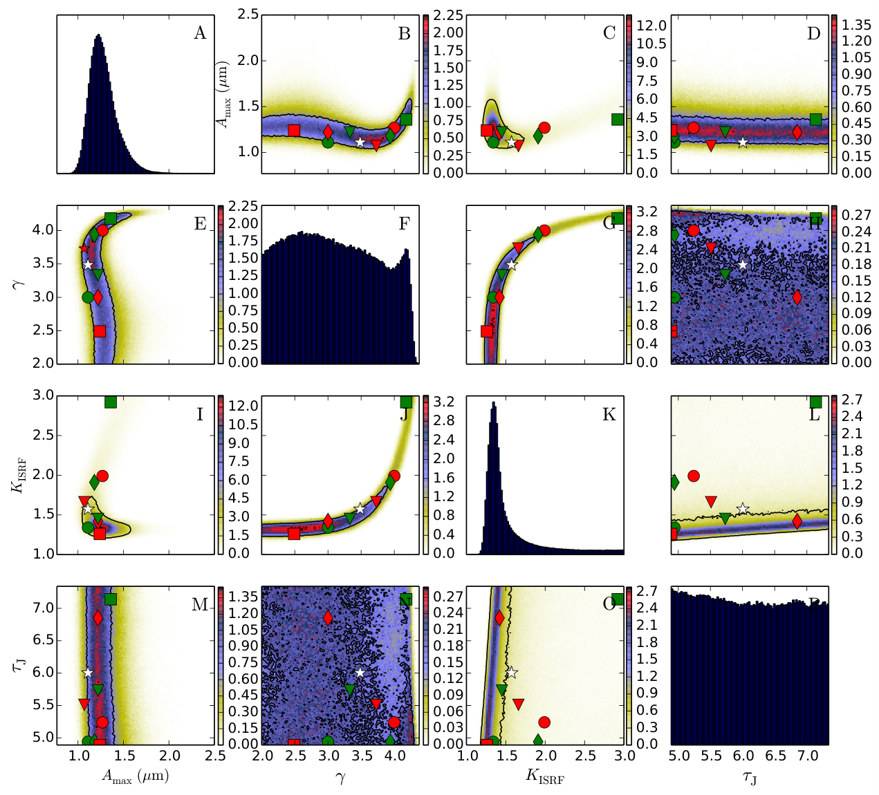
Figure 10 shows the marginalised probability distributions of a one dimensional model cloud with $\tau_{J}=6$. An isotropic radiation field is used in the scattering computations. The distributions are normalised and we only compare the relative probabilities of the different parameter combinations. Figure 10 indicates a strong dependence between $\gamma$ and $K_{\rm ISRF}$. The dependence between parameters is also seen in the ($\gamma$, $\tau$) projection as a strong cut-off at high $\gamma$. Thus, to be able to determine either the $\gamma$ or $K_{\rm ISRF}$, the values of the other parameters must already be known with good precision. The four-dimensional parameter space is not easily represented with two-dimensional correlation plots. The maximum of the marginalised probability and the projected location of the minimum in the four-dimensional $\chi^{2}$ are both shown.

The assumed error estimates of the intensity values have little effect on the results, apart from the broadening of the distributions. Small variations in the intensities of individual channels do affect the location of the $\chi^{2}$ minimum as can be seen from the locations of the green and red symbols in Fig. 10. Even a moderate change of $\pm$ 10 $\%$ in the intensity of one channel can change the recovered $\chi^{2}$ minimum values of $\gamma$ and $K_{\rm ISRF}$ by up to $\sim$60%. In the fit a change of optical depth can be compensated by a change of the radiation field intensity. For further computations we use a constant value of $\tau_{\rm J}=6$, or $\tau_{\rm J}=2$, since it is possible to derive a reasonable estimate for the optical depth using other methods, for example with observations of background stars (Lombardi & Alves, 2001).

Using an anisotropic radiation field in the scattering computations (Fig. 25), produces well constrained distributions for both $\gamma$ and $K_{\rm ISRF}$ parameters, but the $A_{\rm max}$ distribution is considerably broader and shifted to higher parameter values.

The analysis of surface brightness data depends on not only the line-of-sight optical depth but also on the cloud morphology. We derive synthetic observations from a three dimensional prolate ellipsoidal model cloud (see Sect. 2.1). The dust parameters were set to $A_{\rm max}=1.18$, $\gamma=3.67$, and $K_{\rm ISRF}=1.2$ and an anisotropic radiation field corresponding to the Taurus case (see Malinen et al. (2013)) is used in the scattering computations. The optical depth along the line of sight is set to $\tau_{\rm J}=6.0$.

For the analysis of these synthetic observations, one needs the relation between dust parameters and the surface brightness. This can be derived with radiative transfer modelling but it further depends on assumptions of the cloud shape. We compare two cases where the relationship is derived with radiative transfer modelling where one views a three dimensional prolate ellipsoidal cloud either along its major axis or its minor axis, see Fig. 12. In the following we refer to these as the major axis and minor axis radiative transfer models, respectively. In these radiative transfer calculations the model cloud has an axis ratio of 3 and the line-of-sight optical depth is in both cases set to $\tau_{\rm J}=6$. When the radiative transfer model is used to calculate surface brightness along its minor axis, it suffers from more extinction in the direction perpendicular to the line-of-sight (where the full optical depth through the cloud is $\tau_{\rm J=18}$). This affects the radiation field inside the radiative transfer model and thus also leads to a different mapping between the dust parameters and the predicted surface brightness. This is expected to bias the estimates derived for the dust parameters. In the scattering computations we use the anisotropic radiation field. The synthetic observations correspond to the case where the radiative transfer model is viewed along its minor axis. The results with $\sigma_{\rm NIR}=10\%$ are shown in Fig. 11, which shows that the assumptions of the radiative transfer models have a clear effect on the estimated dust parameters.

The one-dimensional probability distributions (the minor axis case) of both $\gamma$ and $K_{\rm ISRF}$ are not concentrated around the parameter values that were used to derive the synthetic observations. The maximum of the two-dimensional probability distribution of $\gamma$ and $K_{\rm ISRF}$ are centred around $\gamma=4.1$, $K_{\rm ISRF}=1.0$. However, the maxima of the one dimensional $A_{\rm max}$ distribution and the $\chi^{2}$ minimum are well matched with the input parameter values but the mode of the marginalised probability distributions significantly differs from the location of the $\chi^{2}$ minimum. In the major axis case, the probability of larger grains is increased significantly as the $A_{\rm max}$ distribution is shifted to $A_{\rm max}>1.5\mu$m and the peak of the $\gamma$ distribution is shifted from $\gamma\sim 4.3$ to $\gamma\sim 4.1$. On the other hand, the strength of the radiation field has decreased by $\sim 30\%$.

Increasing the uncertainty of the surface brightness observations, $\sigma_{\rm NIR}=20\%$, only broadens the resulting probability distributions. Similarly, changes of the asymmetry parameter $g$ do not produce noticeable changes compared to Fig. 11.

If $K_{\rm ISRF}$ is fixed to a constant value (Fig. 13), the marginalised probability distributions and the $\chi^{2}$ minimum match the used parameter values with much higher precision.

Shown in Fig. 14 are the results when the albedo is changed by $\pm$10%, in the scattering simulations, however, for the parameter estimation we use the unmodified albedo. Changes in the albedo have a clear effect to the parameter distributions. Increasing the albedo of the grains shifts the peak of the $A_{\rm max}$ distribution from $A_{\rm max}\sim 1.0$ $\mu$m to $A_{\rm max}\sim 1.5$ $\mu$m, and decreases the probability of $\gamma<3.5$. Thus, the maximum grain size is increased but the relative amount of large grains is decreased. On the other hand, with higher albedo, the strength of the required radiation field decreases from $K_{\rm ISRF}\sim 1.3$ to $K_{\rm ISRF}\sim 0.7$.

In this section, we analyse the NIR observations of the Taurus filament described in Appendix A. We use the minor axis cloud model described in Sect. 3.3. For the optical depth of the J band we use values of $\tau_{J}=6.0$ and $\tau_{J}=2.0$. The surface brightness and optical depth values derived for both cases are shown in Table 1. Unless otherwise specified, we use the $r_{\rm Si}$=0.5 ratio.

Based on our simulations, strong correlations between the dust parameters are evident as changes in one parameter affect the other parameters. The $K_{\rm ISRF}$ and $\tau_{\rm J}$ can not be constrained simultaneously, as changes in the optical depth can be compensated by changes in the strength of the radiation field. Similarly, increasing the $K_{\rm ISRF}$ will be shift the $\gamma$ distribution to lower values, as in many of our simulations both parameters tend to have long tails. On the other hand, the colour of the NIR-MIR spectra is affected by changes in the $A_{\rm max}$ and $\gamma$. Furthermore, assumptions of the morphology of the cloud can change the estimated dust parameters significantly.

To categorise the parameter distributions, we use relative uncertainty

where $x$ is the dust parameter, $Q_{1}$ and $Q_{3}$ are values of the first and third quartile, $Q_{2}$ is the median, and the factor 1.349 is the scaling between the interquartile range $Q_{3}-Q_{1}$ and the standard deviation in case of a normal distribution.

For the probability distributions that are derived using the synthetic observations, we define the difference between the median of the distribution and the correct value of the dust parameter

In the computations with the synthetic observations, the probability distributions of $A_{\rm max}$ and $K_{\rm ISRF}$ have a clear peak near the correct values used to derive the observations. For the model shown in red in Fig. 10, the $\Delta(A_{\rm max})=13\%$ and $r(A_{\rm max})=25\%$ and the $\Delta(K_{\rm ISRF})=-1.7\%$ and $r(K_{\rm ISRF})=61\%$. However, the $\gamma$ distribution of the model does not have a clear peak around the true value, however, the resulting $\Delta(\gamma)=-0.5\%$ and $r(\gamma)=24\%$. The difference between assuming a major axis or minor axis radiative transfer model can change the estimated amount of large grains, by changing the $A_{\rm max}$ by up to $\sim 30\%$ and $\gamma$ by up to $\sim 10\%$ and affect the estimated $K_{\rm ISRF}$ by up to $\sim 30\%$.

Small variations in the optical properties of the dust grains are reflected to the derived dust parameters. If the albedo of the grains is increased by $10\%$ in the scattering simulations the probability of larger grain sizes increases as seen in Fig. 14. The peak of the $A_{\rm max}$ distribution shifts from $A_{\rm max}\sim 1$ $\mu$m up to $A_{\rm max}\sim 1.5$ $\mu$m, and the probability of grain sizes in excess of 2 $\mu$m increases. However, the increase in albedo in the simulations also increases the probability of $\gamma>3.5$ and decreases the strength of the required radiation field. Thus, although the maximum grain size increases, the relative amount of large grains is decreased. Similarly the $\Delta(A_{\rm max})=27\%$ and $r(A_{\rm max})=26\%$, whereas for the $\gamma$ distribution the $\Delta(\gamma)=5.2\%$ and $r(\gamma)=18\%$ and for the $K_{\rm ISRF}$ distribution the $\Delta(K_{\rm ISRF})=5.8\%$ and $r(K_{\rm ISRF})=71\%$. Decreasing the albedo by $10\%$ results in deviations between the correct values and the median values of $\Delta(A_{\rm max})=1.4\%$, $\Delta(\gamma)=-0.8\%$, and $\Delta(K_{\rm ISRF})=14\%$ and the relative uncertainties are $r(A_{\rm max})=23\%$, $r(\gamma)=28\%$, and $r(K_{\rm ISRF})=38\%$.

The changes in the shape of the $A_{\rm max}$ and $\gamma$ distributions are related to the way radiation is scattered by the grains. A higher albedo decreases the absorption efficiency of the dust grains resulting in a spectra that is bluer compared to the reference spectra, thus, larger grain sizes are needed. However, because of the increased scattering efficiency, the amount of large grains is smaller. Shown in Fig. 20 are the spectra computed from three different dust models by varying either the $A_{\rm max}$ or $\gamma$ parameter. Changes in the $A_{\rm max}$ have stronger effect on the resulting intensities compared to changes in $\gamma$.

An error of 10% in the intensity of a single band (see Fig. 10) affects the derived value of $A_{\rm max}$ by $<10\%$, but, the derived value of $K_{\rm ISRF}$ can change by up to 60%. Uncertainty in the observed H or K band intensity affects the derived parameter values more than changes in J or 3.6 $\mu$m bands.

Many of our MCMC computations show a high probability for grain sizes in clear excess of 2 $\mu$m, but the estimated size distribution can also be changed by using different type of grains. We have used a simple model with bare silicate and carbon grains, thus, in order to increase the surface brightness of scattered light at longer wavelengths the maximum grain size has to be increased. However, the scattering properties of the dust grains can be changed by including ice mantles, coagulation, or by changing the surface composition (e.g. hydrogen rich carbon mantles) of the grains, thus increasing the scattering efficiency without increasing the grain sizes (Ysard et al., 2016; Jones et al., 2016).

Coagulation and formation of ice mantles will change the size distribution, decreasing the amount of small grains. As seen in 2, the small grains can cause significant amount of absorption, and thus, reduce the amount of photons available for scattering. We have run separate computations, where we have removed all grains smaller than 20 nm from the dust model. The results of the simulations, using the synthetic observations of the minor axis case (see Fig. 11) and assuming $\tau_{\rm J}=6$, are shown in Fig. 21. Compared to the minor axis case (red lines), removing small grains from the model that is used to fit the synthetic observations (purple lines) does have an effect on the resulting marginalised probability distributions but it is not large. The peak of the $\gamma$ distribution is shifted to a higher value of $\gamma=4.5$ and the $K_{\rm ISRF}$ distribution has a upper limit of $K_{\rm ISRF}=2$.

The changes in $A_{\rm max}$ and $\gamma$ affect the fraction of mass in large grains (Fig. 22)

where $m(a>0.25\mu\rm m)$ is the mass of grains larger than 0.25 $\mu$m and $m$ is the total mass. In all cases, the mass fraction in large grains increases sharply when the value of $\gamma$ decreases. In the case of lower optical depth, the $f_{\rm BG}$ is higher compared to the $\tau_{\rm J}=6$ case. However, based on the MCMC results, the probability that a diffuse line-of-sight would have more large grains than a optically thicker line-of-sight is $p(f_{\rm BG}(\tau_{\rm J}=6)>f_{\rm BG}(\tau_{\rm J}=2))=25\%$. The result is not statistically meaningful, thus, the evidence for a high amount of large grains towards the $\tau_{\rm J}=2$ line-of-sight is not very strong.

In many of our computations, the estimated $K_{ISRF}$ has a clear peak around $\sim 1.1$, but $K_{\rm ISRF}$ could also be significantly higher. However, if the radiation field and optical depth can be constrained, for example setting a constant value for $K_{\rm ISRF}$ and $\tau_{\rm J}$ (Fig. 13) results in well constrained parameter distributions for both $A_{\rm max}$ and $\gamma$ with $\Delta(A_{\rm max})=3.4\%$, $r(A_{\rm max})=20\%$ and $\Delta(\gamma)=0.2\%$, $r(\gamma)=3.2\%$. Assuming a prior 20% uncertainty in $K_{\rm ISRF}$ and $\tau_{\rm J}$, results in $A_{\rm max}$ and $\gamma$ distributions that are broader ($\Delta(A_{\rm max})=4.2\%$, $r(A_{\rm max})=18\%$ and $\Delta(\gamma)=7.9\%$, $r(\gamma)=17\%$, respectively).

The analysis of the computations where the synthetic observations are used shows that on average the $r(A_{\rm max},\gamma)\sim 25\%$, whereas the $r(K_{\rm ISRF})$ is $\sim 45\%$ on average. However, the $r(K_{\rm ISRF})$ can reach values as high as $\sim 70\%$.

As seen in the synthetic observations, the optical depth of the cloud is not well constrained by studying only the scattered light. This is related to the saturation of the surface brightness, and the degeneracy between radiation field intensity and dust opacity as changes in opacity can be negated with changes in the strength of the radiation field. When possible, analysis should include external constraints on the opacity or the radiation field that can be obtained from dust emission or directly from extinction measurements.

If the radiation field strength and the optical depth of the cloud can be constrained, the surface brightness ratio between J and K bands can be used to place useful constraints on the dust properties. However, for diffuse regions, the location of the cloud with respect to the source of illumination should be taken into account since differences of the asymmetry parameter can change the relative brightness between the J and K bands, however, the effect of the asymmetry parameter also depends on the optical depth of the cloud.

We have assumed that the background in Eq. 2 is truly a background and there is no emission from between the cloud and the observer. Emission originating between the cloud and the observer causes error in the assumed transmitted radiation $I_{\rm bg}e^{-\tau}$ and thus also in the deduced colour of the scattered component. A more detailed radiative transfer study is needed to explore the effects arising from the surrounding medium. In our simulations we have used smooth spherical and ellipsoidal cloud models but have not considered effects of small-scale density inhomogeneities that could affect the way radiation penetrates the cloud. Furthermore, we have used a constant scaling for the strength of the radiation field $K_{\rm ISRF}$, thus we have not considered possible changes in the shape of the background spectra.

The $K_{\rm ISRF}$ distribution tends to have a long tail towards higher values, while the powerlaw exponent of the grain size distribution $\gamma$ has a tail towards lower values. The tails are probably caused by the chosen prior distributions of the parameters. Allowing the $K_{\rm ISRF}$ to have values larger than 3.0, would likely allow the $\gamma$ distribution to reach even smaller values.

The position of the $\chi^{2}$ minimum does not usually coincide exactly the maximum of the marginalised probability. The three dimensional function $\chi^{2}(A_{\rm max},\gamma,K_{\rm ISRF})$ is complex, and the minimum is shallow. Furthermore, the values of the $\chi^{2}$ function are computed from simulations that have noise, thus the actual location of the computed $\chi^{2}$ minimum can be affected by noise.

The marginalised probability distributions are projections of a three dimensional distribution. Thus it is possible that the $\chi^{2}$ minimum of the three dimensional distribution does not match with the maximum of the projected two dimensional probability. Furthermore, using higher error estimates for the surface brightness data can have a significant effect on the location of the $\chi^{2}$ minima. The instability of the $\chi^{2}$ minima, seems analogous with the color temperature and spectral index, $T_{\rm C}$-$\beta_{\rm spec}$, plane. As discussed by Juvela & Ysard (2012), even a slight change in the weighting of the frequency points or in the noise can significantly shift the location of the global minimum. High uncertainties make the $\chi^{2}$ minima shallow and, together with noise, contribute to ambiguity in the actual location of the $\chi^{2}$ minima.

As an example we have analysed observations of a filament in the Taurus molecular cloud, TMC-1N. Our cloud model is an ellipsoid with a $3:1$ ratio between the major and minor axes, illuminated by an anisotropic radiation field derived from the DIRBE observations and viewed along one of the minor axes. The optical depth of the model cloud along the line-of-sight is set to $\tau_{\rm J}=6$ or $\tau_{\rm J}=2$. Based on our analysis for the TMC-1N $\tau_{J}=6$ position, a maximum grain size of $A_{\rm max}\sim 1.2$ $\mu$m and $\gamma>4$ are most probable, with an average relative uncertainty of $r(A_{\rm max})=36\%$, $r(\gamma)=22\%$, and $r(K_{\rm ISRF})=38\%$. However, there is a considerable possibility of grains larger than $A_{\rm max}>2.0$ $\mu$m. The mass weighted average grain size is $\langle a_{\rm m}\rangle=0.113$, which is higher than $\langle a_{\rm m}\rangle=0.089$ of the MRN distribution. The anisotropic radiation field derived from the DIRBE observations is sufficient to reproduce the observed surface brightness values.

Shown in Fig. 23, is a cut of the marginalised probability distribution around the $\chi^{2}$ minimum for the TMC-1N $\tau_{J}=6$ position with $r_{\rm Si}$=0.5 and assuming $\sigma_{\rm NIR}=10\%$, see Fig. 15. In all of the panels, the $\chi^{2}$ minimum matches with the maximum of the marginalised probability.

If one assumes larger observational uncertainties $\sigma_{\rm NIR}=20\%$, the resulting parameter distributions are smoother and broader, with an average relative uncertainty of $r(A_{\rm max})=26\%$, $r(\gamma)=24\%$, and $r(K_{\rm ISRF})=30\%$. However, the increased $\sigma_{\rm NIR}$, of both TMC-1N $\tau_{J}=6$ and $\tau_{J}=2$ positions, can also change the interpretation of the dust properties. For example, with a lower $\sigma_{\rm NIR}$, the $A_{\rm max}$ distributions of Fig. 15 shows a clear peak around $\sim 1$ $\mu$m, and a tail towards higher parameter values and a $r=37\%$. Adopting a higher $\sigma_{\rm NIR}$ shifts the peak of $A_{\rm max}$ distribution to higher value, $\sim 1.5$ $\mu$m, causes a significant increase for $A_{\rm max}>1.5$ $\mu$m, and decreases $r(A_{\rm max})$ to $25\%$. With lower uncertainties the $\gamma$ distribution has a plateau or a bump around 3.5 and the $r(\gamma)=22\%$, whereas with higher $\sigma_{\rm NIR}$ the distribution is smoother and the $r(\gamma)=24\%$.

The 3.6 $\mu$m band will place more constraints on the probability distributions, significantly increasing the probability of $A_{\rm max}>1.5\mu$m with $r(A_{\rm max})=30\%$, $r(\gamma)=25\%$, and $r(K_{\rm ISRF})=56\%$ However, caution should be taken with the 3.6 $\mu$m band. To derive reliable estimates for the dust parameters the fraction of emission in the observed surface brightness should be know to a reasonable accuracy.

With lower optical depth, case $\tau_{\rm J}=2.0$, the parameter distributions are significantly narrower with average $r(A_{\rm max},\gamma,K_{\rm ISRF})<10\%$. The $\gamma$ values are smaller than $\sim 3.8$ and the values of $A_{\rm max}$ are concentrated to values larger than 2 $\mu$m. However, the opposite would be expected, since for a more diffuse line-of-sight, the dust grains are thought to be less evolved, and thus, smaller values of $A_{\rm max}$ and larger values of $\gamma$ would be expected. Increasing the $\sigma_{\rm NIR}$ pushes the $\gamma$ distribution to lower value $\gamma\sim 2.4$. The change in the $\gamma$ distribution is likely related to the shape of the $\chi^{2}$ space and changes in the assumed error estimates can also strongly affect the way the priori affect the posterior probability distributions.

The $K_{\rm ISRF}$ distribution is slightly lower in the case $\tau_{\rm J}=2.0$, although the radiation field there should be less attenuated. A region with lower optical depth could be used to constrain the strength of the radiation field. For case $\tau_{\rm J}=2.0$, the intensity of the 3.6 $\mu$m band is low, which introduces additional uncertainty to the derived dust parameters.