跳到论文正文
W Papers独立论文阅读器 arXiv:1802.07382 论文正文 计算阅读时间 · 0%
引用这篇论文根据当前论文元数据生成,正式投稿前建议核对。


License: arXiv.org perpetual non-exclusive license
arXiv:1802.07382v3 [cs.LG] 23 Dec 2021

Generic Coreset for Scalable Learning of Monotonic Kernels: Logistic Regression, Sigmoid and more

Elad Tolochinsky Affiliation: University of Haifa, Israel Email: eladt26@gmail.com    Ibrahim Jubran Affiliation: University of Haifa, Israel Email: ibrahim.jub@gmail.com    Dan Feldman Affiliation: University of Haifa, Israel Email: dannyf.post@gmail.com
Abstract

Coreset (or core-set) is a small weighted subset QQ of an input set PP with respect to a given monotonic function f:ℝ→ℝf:\mathbb{R}\to\mathbb{R} that provably approximates its fitting loss ∑p∈Pf⁡(p⋅x)\sum_{p\in P}f(p\cdot x) to any given x∈ℝdx\in\mathbb{R}^{d}. Using QQ we can obtain approximation of x∗x^{*} that minimizes this loss, by running existing optimization algorithms on QQ. In this work we provide: (i) A lower bound which proves that there are sets with no coresets smaller than n=|P|n=|P| for general monotonic loss functions. (ii) A proof that, under a natural assumption that holds e.g. for logistic regression and the sigmoid activation functions, a small coreset exists for any input PP. (iii) A generic coreset construction algorithm that computes such a small coreset QQ in O⁡(n​d+n​log⁡n)O(nd+n\log n) time, and (iv) Experimental results with open-source code which demonstrate that our coresets are effective and are much smaller in practice than predicted in theory.

1 Introduction

Traditional algorithms in computer science and machine learning are usually tailored to handle off-line finite datasets that are stored in memory. However, many modern systems do not use this computational model. For example, GPS data from millions of smartphones, high definition images, YouTube videos, Twitter tweets, or audio signals from smart homes arrive in a streaming fashion. The era of Internet of Things (IoT) provides us with wearable devices and mini-computers that collect data sets that are being gathered by ubiquitous information-sensing mobile devices and wireless sensor networks [19, 31, 14].

Challenges. Using such devices and networks pose a series of challenges:
(i) Limited memory. In such systems, the input is an infinite stream of batches that may grow in practice to petabytes of raw data, and cannot be stored in memory. Hence, only one-pass over the data and small memory are allowed.
(ii) Parallel computations. To leverage the power of multithreading and multiple processing units (as in GPUs), we are required to design variants of our algorithms which can run in parallel.
(iii) Distributed computations. If the dataset is distributed among many machines, e.g. on a “cloud", there is an additional problem of non-shared memory, which may be replaced by expensive and slow communication between the machines.

Weak or no theoretical guarantees. Due to the modern computation models above, learning trivial properties of the data may become non trivial, as stated in [14]. These problems are especially common in machine learning applications, where the common optimization problems and models may be, already in the off-line settings NP-hard. The result is neglecting, in some sense, decades of theoretical computer science research, and replacing it by fast heuristics and ad-hoc rules, which are easy to implement under the above constrains, and provide reasonable results. Those heuristics, however, have no theoretical guarantees, either as of running time or of global optimality.

1.1 Coresets

Coresets suggest a natural solution or at least a very generic approach to address the above challenges without re-inventing computer science. Coresets have some promising theoretical guarantees, while still leveraging the success of existing heuristics. Instead of designing, from scratch, a new algorithm to solve the problem at hand, the idea is to provably summarize the data into a small representative subset, and to prove that applying existing algorithms, both heuristics and provable methods, on this small summarizations, will yield an output which approximates the result of running the same algorithms on the original (full) data.

In this paper we focus on coresets for monotonic continuous functions, that is: we assume that we are given a set PP of nn points in ℝd\mathbb{R}^{d}, and a non-decreasing monotonic functions f:ℝ→ℝ>0f:\mathbb{R}\to\mathbb{R}_{>0}. For a given error parameter ε∈(0,1)\varepsilon\in(0,1), we wish to compute an ε\varepsilon-coreset Q⊆PQ\subseteq P, with a weight function u:Q→[0,∞)u:Q\to[0,\infty) that provably approximates the fitting cost of PP for every x∈ℝdx\in\mathbb{R}^{d}, up to a multiplicative factor of 1±ε1\pm\varepsilon, i.e., (1−ε)​∑p∈Pf⁡(p⋅x)≤∑p∈Qw⁡(p)​f​(p⋅x)≤(1+ε)​∑p∈Pf⁡(p⋅x)(1-\varepsilon)\sum_{p\in P}f(p\cdot x)\leq\sum_{p\in Q}w(p)f(p\cdot x)\leq(1+\varepsilon)\sum_{p\in P}f(p\cdot x). Although it seems rather theoretic, many real world problems can be formulated using such functions, including the Sigmoid, Logistic regression, SVM, Linear classifiers, and Gaussian Mixture Models; see examples in [10].

Coresets and machine learning. We can use the notion of coresets as described above for improving the performance of machine learning algorithms. Most machine learning algorithms essentially solve an optimization problem over some set of training data. By constructing a coreset for this training data, we can: (i) greatly reduce the time it takes to train a model, simply by training it on the (small) coreset, and (ii) allow support for streaming, parallel, and distributed data. Although the coreset provides guarantees for the approximation of the MSE of the training data, it can be shown that for some problems, a coreset can also provide guarantee for the approximations of the generalizations error. For example, when using Bayesian inference, it was shown in [20] that a model which is based on coreset for the log likelihood function, has a marginal likelihood which is guaranteed to approximate the true marginal likelihood. The same can be shown for maximum likelihood estimation. The popular measure for the goodness of fit of an estimator is the the log-likelihood ratio: ln⁡Λ⁡(θ^)=ℒ⁡(θ^)−supθ∈Θℒ⁡(θ)\ln\Lambda(\hat{\theta})=\mathcal{L}(\hat{\theta})-\sup_{\theta\in\Theta}\mathcal{L}(\theta). The log-likelihood ratio of a model which is based on a coreset, uniformly approximates the log-likelihood ratio of the full model. Furthermore, coresets have been shown to practically improve the generalization error for machine learning algorithms [20, 11, 28]

1.2 Our contribution

(i) We provide an impossibility bound that proves that, for non-decreasing monotonic loss function, there are no small coresets in general. We do this by providing an example of an input set of points PP, for which no coreset of size smaller than |P||P| exists; see Section 3.

(ii) Following the bound above, we can either give up on the generic coreset paradigm, or add natural assumptions and modifications to the targeted functions ff. In this paper we choose the second option; We add a regularization term to the loss function, which, in most cases, is added anyway to avoid overfitting [30, 2]. In fact, in some cases, this new term is crucial as some functions are minimized only for xx approaching infinity if this term is omitted. For example, the regularization term we add to the sigmoid function is ‖x‖22/k\left\lVert x\right\rVert_{2}^{2}/k, where k>0k>0 defines the trade-off between minimizing the function and the complexity of the set of parameters. While minimizing such functions may still be NP-hard [32], we prove that a small coreset QQ exists for any input set PP, for the sigmoid and logistic regression functions; see Section 5. However, the proof holds for a wider family of functions.

(iii) We provide a generic algorithm that computes the coreset QQ above in O⁡(n​d+n​log⁡n)O(nd+n\log n) time. Unlike most existing works, our algorithm can construct a coreset for the sigmoid and logistic regression functions, as well as a wider set of functions; see Algorithm 1.

(iv) Open source code for our algorithms is given [5], along with extensive experimental results on both synthetic and real-world public datasets; see Section 6.

1.3 Related Work

In [17], Har-Peled shows how to construct a coreset of one dimensional points sets (d=1)(d=1) for sums of single variable real valued functions. In the scope of machine learning most of the research involves clustering techniques [15, 16, 13] and regressions [3, 8, 39]. Several coresets were constructed for unsupervised learning problems including coresets for Gaussian mixture models [11], and SVM [33, 18]. Other works handle general families of supervised learning problems [34, 25].

The work by [20] introduces lower bounds on the total sensitivity of the logistic regression problem that is used in this paper. It also introduces an upper bound for the total sensitivity and coreset size based on kk-clustering coresets. However the bounds hold only for input set PP from very specific distributions (roughly, when PP is well separated into kk clusters).

In [28], a lower bound of Ω⁡(n/log⁡n)\Omega\left(n/\log n\right) points, on the size of a coreset for a two dimensional logistic regression was introduced. To find a coreset, the authors have introduced a measure of the data μ\mu, which depends on the log-ratio between the positive and negative labeled points, and have shown that for data sets in which μ\mu is sufficiently small a coreset of size O⁡(p​o​l​y​(log⁡n))O(poly(\log n)) exist. Instead of imposing assumptions on the above input-related measure, in this work we add a regularization term to the loss function which, as we show, makes the coreset construction task feasible. There does not seem to be a direct relation between our work and the measure μ\mu used in [28].

The main tool of this work uses the unified framework presented in [12], which was recently improved in [4]. We also use the reduction from ℒ∞\mathcal{L}_{\infty} coresets that approximates maxp∈P⁡f⁡(p⋅x)\max_{p\in P}f(p\cdot x) to our ℒ1\mathcal{L}_{1} coreset (sum of loss) which was introduced in [37].

1.4 Paper Organization

Section 2 describes preliminary results which we utilize in our coreset construction algorithm. In Section 3 we give examples of input sets which have no non-trivial coreset (i.e., smaller than the input size), for general monotonic functions. In Section 4 we introduce our main coreset construction algorithm. We then prove the correctness of this algorithm for the sigmoid and logistic regression activation functions. In Section 6 we provide our experimental results along with a discussion.

2 Preliminaries

In what follows we first describe the coreset construction framework of [12]. The framework is based on a non-uniform sampling of the input, according to some importance distribution over the input points. This distribution assigns higher values to points of higher influence on the optimization problem at hand. Now, in order to keep the sample unbiased, the sampled points are reweighted reciprocal to their sampling probability. To quantify the influence of a single point on the optimization problem, Feldman and Langberg suggested in [23] a term called sensitivity, which we define later in this section. Using the sensitivity, a sampling-based coreset can be constructed, whose size depends on the total sensitivity over the input points, a complexity measure of the family of models, called the VC-dimension, and an error parameter ε∈(0,1)\varepsilon\in(0,1) that controls the trade-off between coreset size and approximation accuracy. Bounding the VC-dimension of the loss functions handled in this paper is straightforward; see formal details in Section D at the supplementary material. Hence, the majority of the paper is devoted to bound the sensitivity of each point.

We now formally define the sensitivity of every input point, with respect to a given problem at hand.

Definition 1 (Sensitivity [12, 23]).

Let (P,w,X,c)(P,w,X,c) be a tuple called query space, where PP is a finite set of elements, w:P→[0,∞)w:P\to[0,\infty) is a weight function, XX is a set called queries (models), and c:P×X→[0,∞)c:P\times X\to[0,\infty) is a loss function. The sensitivity of a point 𝐩∈P\boldsymbol{p}\in P with respect to (P,w,X,c)(P,w,X,c) is defined as

s⁡(p):=sP,w,X,c​(𝒑)=sup𝒙∈Xw⁡(𝒑)​c​(𝒑,𝒙)∑𝒑′∈Pw⁡(𝒑′)​c​(𝒑′,𝒙),s(p):=s_{P,w,X,c}\left(\boldsymbol{p}\right)=\sup_{\boldsymbol{x}\in X}\frac{w\left(\boldsymbol{p}\right)c\left(\boldsymbol{p},\boldsymbol{x}\right)}{\sum_{\boldsymbol{p^{\prime}}\in P}w\left(\boldsymbol{p^{\prime}}\right)c\left(\boldsymbol{p^{\prime}},\boldsymbol{x}\right)},

where the supremum is over every 𝐱∈X\mathbf{x}\in X such that the denominator is positive . The total sensitivity of the query space is denoted by t⁡(P):=t⁡(P,w,X,c)=∑𝐩∈Ps⁡(𝐩)t(P):=t(P,w,X,c)=\sum_{\boldsymbol{p}\in P}s(\boldsymbol{p}).

One of the contributions of [12] is to establish a connection to the theory of range spaces and the well known VC-dimension. Informally, the (VC) dimension of a given problem is a measure of its combinatorial complexity [1]. For completeness, a formal definition is given in the supplementary material; see Section D.

Feldman and Langberg also show how to compute, without further assumptions, a small weighted set (Q,u)(Q,u), where Q⊆PQ\subseteq P, that will approximate the total cost C⁡(P,w,𝒙)C\left(P,w,\boldsymbol{x}\right) of the input (P,w)(P,w), for every query 𝒙∈X\boldsymbol{x}\in X, up to a multiplicative factor of 1±ε1\pm\varepsilon. Such a set, which we call a coreset, is defined as follows.

Definition 2 (ε\varepsilon-coreset).

Let (P,w,X,c)\left(P,w,X,c\right) be a query space (see Definition 1), and ε∈(0,1)\varepsilon\in(0,1) be an error parameter. An ε\varepsilon-coreset for (P,w,X,c)\left(P,w,X,c\right) is a weighted set (Q,u)\left(Q,u\right) such that for every 𝐱∈X\boldsymbol{x}\in X,

|∑𝒑∈Pw⁡(𝒑)​c​(𝒑,𝒙)−∑𝒒∈Qu⁡(𝒒)​c​(𝒒,𝒙)|≤ε⋅∑𝒑∈Pw⁡(𝒑)​c​(𝒑,𝒙).\left|\sum_{\boldsymbol{p}\in P}w\left(\boldsymbol{p}\right)c\left(\boldsymbol{p},\boldsymbol{x}\right)-\sum_{\boldsymbol{q}\in Q}u\left(\boldsymbol{q}\right)c\left(\boldsymbol{q},\boldsymbol{x}\right)\right|\leq\varepsilon\cdot\sum_{\boldsymbol{p}\in P}w(\boldsymbol{p})c(\boldsymbol{p},\boldsymbol{x}).

In [12], a lower bound is given for the required coreset size, as a function of the total sensitivity t⁡(P)t(P). This bound was later made tighter in [4]. The following theorem describes the random sampling scheme for coreset construction using the sensitivity framework, and describes the required sample (coreset) size.

Theorem 3 (coreset construction [4, 12]).

Let (P,w,X,c)\left(P,w,X,c\right) be a query space of VC-dimension dd and total sensitivity tt. Let ε,δ∈(0,1)\varepsilon,\delta\in(0,1). Let QQ be a random sample of |Q|≥10​tε2​(d​log⁡t+log⁡(1δ))\left|Q\right|\geq\frac{10t}{\varepsilon^{2}}\left(d\log t+\log\left(\frac{1}{\delta}\right)\right) i.i.d points from PP, such that every 𝐩∈P\boldsymbol{p}\in P is sampled with probability 1t⋅sP,w,X,c​(𝐩)\frac{1}{t}\cdot s_{P,w,X,c}\left(\boldsymbol{p}\right). Let u⁡(𝐩)=t⋅w⁡(𝐩)sP,w,X,c​(𝐩)​|Q|u\left(\boldsymbol{p}\right)=\frac{t\cdot w\left(\boldsymbol{p}\right)}{s_{P,w,X,c}\left(\boldsymbol{p}\right)\left|Q\right|} for every 𝐩∈Q\boldsymbol{p}\in Q. Then, with probability at least 1−δ1-\delta, (Q,u)\left(Q,u\right) is an ε\varepsilon-coreset of (P,w,X,c)\left(P,w,X,c\right).

3 Lower Bounds

In what follows, we consider query spaces (P,w,ℝd,c)(P,w,\mathbb{R}^{d},c), where c⁡(𝒙,𝒑)=f⁡(𝒙⋅𝒑)c(\boldsymbol{x},\boldsymbol{p})=f(\boldsymbol{x}\cdot\boldsymbol{p}) for some non-decreasing monotonic function ff. We prove that not all such query spaces admit a non-trivial coreset, by providing an example of an input sets PP for which every coreset must be of size |P||P|.

No coreset.

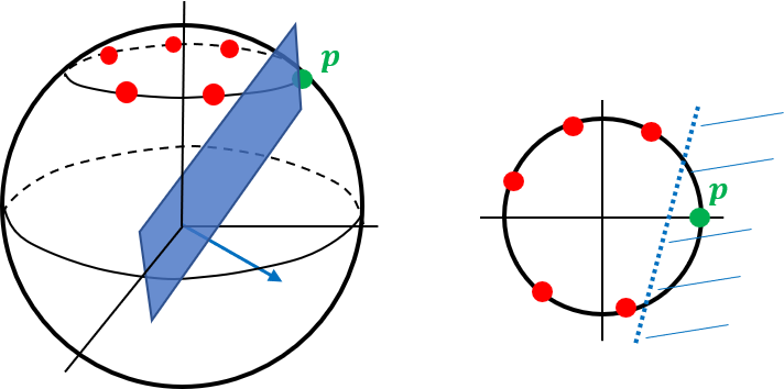
Consider a 2-dimensional circle C⊆ℝ3C\subseteq\mathbb{R}^{3} in 33-dimensional space, which is the intersection of the unit sphere and a non-affine plane (does not pass through the origin) that is parallel to the X​YXY plane. For every point 𝒑∈P\boldsymbol{p}\in P, let π𝒑\pi_{\boldsymbol{p}} be a plane in ℝ3\mathbb{R}^{3} that passes through the origin which isolates 𝒑\boldsymbol{p} from the rest of the set, and let 𝒙𝒑\boldsymbol{x_{p}} be a vector orthogonal to π𝒑\pi_{\boldsymbol{p}}, such that 𝒑⋅𝒙𝒑>0\boldsymbol{p}\cdot\boldsymbol{x_{p}}>0; see Fig 1. Such a plane exists since the points are on a 2D circle that is not centered around the origin.

Now, for intuition, consider the logistic regression cost function: c⁡(𝒙,𝒑)=log⁡(1+e𝒑⋅𝒙)c(\boldsymbol{x},\boldsymbol{p})=\log(1+e^{\boldsymbol{p}\cdot\boldsymbol{x}}). Let 𝒑∈P\boldsymbol{p}\in P and let 𝒙𝒑\boldsymbol{x_{p}} be the query vector orthogonal to the plane π𝒑\pi_{\boldsymbol{p}} which separates 𝒑\boldsymbol{p} from the rest of the set. Since 𝒑\boldsymbol{p} is the only point on the positive side of 𝒙𝒑\boldsymbol{x_{p}}, it holds that 𝒑⋅𝒙𝒑>0\boldsymbol{p}\cdot\boldsymbol{x_{p}}>0 whereas for every other point 𝒑′\boldsymbol{p^{\prime}}, 𝒑′⋅𝒙𝒑<0\boldsymbol{p^{\prime}}\cdot\boldsymbol{x_{p}}<0. Moreover as ‖𝒙𝒑‖\left\lVert\boldsymbol{x_{p}}\right\rVert grows, 𝒑⋅𝒙𝒑\boldsymbol{p}\cdot\boldsymbol{x_{p}} goes to ∞\infty and 𝒑′⋅𝒙𝒑\boldsymbol{p^{\prime}}\cdot\boldsymbol{x_{p}} grows to −∞-\infty. Thus the cost c⁡(𝒙𝒑,𝒑)=log⁡(1+e𝒑⋅𝒙𝒑)c(\boldsymbol{x_{p}},\boldsymbol{p})=\log(1+e^{\boldsymbol{p}\cdot\boldsymbol{x_{p}}}) of 𝒑\boldsymbol{p}, goes to ∞\infty and the cost of every other point goes to 00. Therefore, 𝒑\boldsymbol{p} has a sensitivity of 11. In this case, intuitively, every coreset must include 𝒑\boldsymbol{p} or else it cannot provide a good approximation to the cost of the original (full) set. Since this argument holds for every 𝒑∈P\boldsymbol{p}\in P, any coreset for PP must include all points in PP. Thus, no non-trivial coreset exists in this case. Putting, it differently, the above discussion shows that if the sensitivity of every point in PP is 11 then the size of every coreset is Ω⁡(n)\Omega(n); see Lemma 11 in the supplementary material for a formal statement.
Refer to caption
Figure 1: (Left): A set of points PP in ℝ3\mathbb{R}^{3} (red and green points), a plane π𝒑\pi_{\boldsymbol{p}} separating pp from P∖{p}P\setminus\left\{p\right\} and the vector 𝒙𝒑\boldsymbol{x_{p}} orthogonal to π𝒑\pi_{\boldsymbol{p}}. (Right): A top-down view of the data on the left. The dotted line ℓ\ell is the intersection of π𝒑\pi_{\boldsymbol{p}} and the plane containing PP. All the points to the right (left) of ℓ\ell are projected onto the positive (negative) side of 𝒙𝒑\boldsymbol{x_{p}}.

Note that the above holds true not only for logistic regression but for any function ff that satisfies limx→∞f⁡(−x)f⁡(x)=0\lim_{x\rightarrow\infty}\frac{f\left(-x\right)}{f\left(x\right)}=0. This is formally stated in the following theorem. A formal proof is given in Section A of the supplementary material.

Theorem 4.

Let f:ℝ→(0,∞)f:\mathbb{R}\rightarrow\left(0,\infty\right) be a non-decreasing monotonic function that satisfies limx→∞f⁡(−x)f⁡(x)=0\lim_{x\rightarrow\infty}\frac{f\left(-x\right)}{f\left(x\right)}=0, and let c⁡(𝐱,𝐩)=f⁡(𝐱⋅𝐩)c\left(\boldsymbol{x},\boldsymbol{p}\right)=f\left(\boldsymbol{x}\cdot\boldsymbol{p}\right) for every 𝐱,𝐩∈ℝd\boldsymbol{x},\boldsymbol{p}\in\mathbb{R}^{d}. Let ε∈(0,1)\varepsilon\in\left(0,1\right), n≥1n\geq 1 be an integer, and w:ℝd→(0,∞)w:\mathbb{R}^{d}\rightarrow\left(0,\infty\right). There is a set P⊂ℝdP\subset\mathbb{R}^{d} of |P|=n|P|=n points such that if (Q,u)(Q,u) is an ε\varepsilon-coreset of (P,w,ℝd,c)\left(P,w,\mathbb{R}^{d},c\right) then Q=PQ=P.

Adding assumptions. The above counter-example and formal claim motivate the necessity of adding assumptions on the loss function, as described in the following section. Mainly, a regularization term needs to be added. This term is usually added anyway, both in theory and in practice, to reduce the complexity of the model and avoid overfitting.

4 Coresets For Monotonic Bounded Functions

From the previous section, we conclude that an additional constraint must be imposed on the problem at hand in order to construct a small coreset. To better understand the required constraint, recall the reason for the lower bound from the example at Section 3; the (problematic) points with sensitivity 1 were the points which had very large values of 𝒙⋅𝒑\boldsymbol{x}\cdot\boldsymbol{p}. This can happen when ‖𝒙‖\left\lVert\boldsymbol{x}\right\rVert is very large or when ‖𝒑‖\left\lVert\boldsymbol{p}\right\rVert is large. For the moment, assume that ‖𝒑‖\left\lVert\boldsymbol{p}\right\rVert is small (we will later see how ‖𝒑‖\left\lVert\boldsymbol{p}\right\rVert affects the size of the coreset). The standard technique for preventing the parameters from growing too large is to add a regularization term, which is widely used in many real world problems [30, 22]. As it happens to be, adding a regularization term also advances us towards our goal of constructing a coreset, as was also noted e.g., in [29, 35]. To see this, consider a regularized variant of the loss function: c⁡(𝒙,𝒑)=f⁡(𝒙⋅𝒑)+‖𝒙‖kc(\boldsymbol{x},\boldsymbol{p})=f\left(\boldsymbol{x}\cdot\boldsymbol{p}\right)+\frac{\left\lVert\boldsymbol{x}\right\rVert}{k}. Since ff is bounded, when ‖𝒙‖\left\lVert\boldsymbol{x}\right\rVert grows to infinity the value of the regularization dominates the loss. Thus, in this case, all points have approximately the same loss, and are all equally unimportant. In other words, the sensitivity of those points can not be 11.

The common case for the value of the regularization parameter kk is k=n1−κk=n^{1-\kappa} for κ∈(0,1)\kappa\in(0,1); see e.g., in [7, 26]. In practice, we observed that the values of kk have only a small effect on the coresets approximation accuracy; see Section 6.

4.1 ℒ∞\mathcal{L}_{\infty} coresets

We now address the common case, in which for some 𝒙∈X\boldsymbol{x}\in X and every two points, 𝒑1\boldsymbol{p}_{1}, 𝒑2∈P\boldsymbol{p}_{2}\in P the values of 𝒑1⋅𝒙\boldsymbol{p}_{1}\cdot\boldsymbol{x} and 𝒑2⋅𝒙\boldsymbol{p}_{2}\cdot\boldsymbol{x} do not greatly differ. To do so, we will reduce our problem to the problem of constructing an ℒ∞\mathcal{L}_{\infty} coreset, which is defined as follows.

Definition 5.

(ℒ∞\mathcal{L}_{\infty} coreset[37]) Let (P,w,X,c) be a query space and ε>0\varepsilon>0. An ε−ℒ∞\varepsilon-\mathcal{L}_{\infty} coreset is a subset Q⊆PQ\subseteq P such that max𝐩∈P⁡c⁡(𝐩,𝐱)≤(1+ε)​max𝐪∈Q⁡c⁡(𝐪,𝐱)\max_{\boldsymbol{p}\in P}c(\boldsymbol{p},\boldsymbol{x})\leq(1+\varepsilon)\max_{\boldsymbol{q}\in Q}c(\boldsymbol{q},\boldsymbol{x}) for every 𝐱∈X\boldsymbol{x}\in X.

We will now focus on constructing an ℒ∞\mathcal{L}_{\infty} coreset. We will then show how to leverage this ℒ∞\mathcal{L}_{\infty} coreset to obtain a coreset as defined in Definition 2.

Consider a monotonic non-decreasing function f:ℝ→(0,M]f:\mathbb{R}\to(0,M], a query 𝒙∈X\boldsymbol{x}\in X and a point 𝒑∈P\boldsymbol{p}\in P such that 𝒑⋅𝒙>0\boldsymbol{p}\cdot\boldsymbol{x}>0. Since ff is a monotonic function, f⁡(0)≤f⁡(𝒑⋅𝒙)f(0)\leq f(\boldsymbol{p}\cdot\boldsymbol{x}). Hence,

max𝒑′∈P⁡f⁡(𝒑′⋅𝒙)≤M=Mf⁡(0)​f​(0)≤Mf⁡(0)​f​(𝒑⋅𝒙),\max_{\boldsymbol{p}^{\prime}\in P}f(\boldsymbol{p}^{\prime}\cdot\boldsymbol{x})\leq M=\frac{M}{f(0)}f(0)\leq\frac{M}{f(0)}f(\boldsymbol{p}\cdot\boldsymbol{x}),

Therefore, for a query 𝒙\boldsymbol{x}, if a point 𝒑\boldsymbol{p} falls on the positive side of the line defined by 𝒙\boldsymbol{x} we can say this point is an ℒ∞\mathcal{L}_{\infty} coreset. But what if the point falls on the negative side of the line? Since ff is monotonic, we know that if 𝒑⋅𝒙<0\boldsymbol{p}\cdot\boldsymbol{x}<0 then, f(𝒑⋅𝒙)<f(−𝒑⋅𝒙)f(\boldsymbol{p}\cdot\boldsymbol{x})<f(-\boldsymbol{p}\cdot\boldsymbol{x}), but if ff is sufficiently “well behaved” then as long as the distance between −𝒑⋅𝒙-\boldsymbol{p}\cdot\boldsymbol{x} and 𝒑⋅𝒙\boldsymbol{p}\cdot\boldsymbol{x} is not too large, then the distance between f(−𝒑⋅𝒙)f(-\boldsymbol{p}\cdot\boldsymbol{x}) and f⁡(𝒑⋅𝒙)f(\boldsymbol{p}\cdot\boldsymbol{x}) is also bounded. Specifically, we can assume there is a constant b>0b>0 such that

f(−𝒑⋅𝒙)<b⋅f(𝒑⋅𝒙)f(-\boldsymbol{p}\cdot\boldsymbol{x})<b\cdot f(\boldsymbol{p}\cdot\boldsymbol{x})

which implies that even if 𝒑\boldsymbol{p} falls on the negative side of the line, then 𝒑\boldsymbol{p} is an ℒ∞\mathcal{L}_{\infty} coreset.

Assumptions and conclusions made so far. Before we conclude the results of this section, we must conduct the assumptions and conclusions we have made so far. We have assumed that the distance between −𝒑⋅𝒙-\boldsymbol{p}\cdot\boldsymbol{x} and 𝒑⋅𝒙\boldsymbol{p}\cdot\boldsymbol{x} is not too large. We can bound the distance as follows:

|−𝒑⋅𝒙−(𝒑⋅𝒙)|=|2𝒑⋅𝒙|≤2‖𝒙‖‖𝒑‖.|-\boldsymbol{p}\cdot\boldsymbol{x}-(\boldsymbol{p}\cdot\boldsymbol{x})|=|2\boldsymbol{p}\cdot\boldsymbol{x}|\leq 2\left\lVert\boldsymbol{x}\right\rVert\left\lVert\boldsymbol{p}\right\rVert.

From the discussion in the beginning of the section, adding regularization will guarantee that ‖𝒙‖\left\lVert\boldsymbol{x}\right\rVert can not grow arbitrarily large. As for the ‖𝒑‖\left\lVert\boldsymbol{p}\right\rVert term, we expect the coreset to be somehow affected by this term in order to ensure the above property. Indeed, this is one of the main terms which affect the sensitivity of the input points. Hence, the final coreset will be more likely to choose points with larger norm.

We conclude that every point 𝒑∈P\boldsymbol{p}\in P is an ε−ℒ∞\varepsilon-\mathcal{L}_{\infty} coreset for sufficiently large ε\varepsilon that depends on properties of the function (M,f⁡(0)M,f(0) and bb) and on ‖𝒑‖\left\lVert\boldsymbol{p}\right\rVert. This is formally stated in the following lemma.

Lemma 6 (ℒ∞\mathcal{L}_{\infty} coresets).

Let P⊂ℝdP\subset\mathbb{R}^{d} be a finite set, M,k>0M,k>0 be constants, f:ℝ→(0,M]f:\mathbb{R}\rightarrow(0,M] be non-decreasing function and g:[0,∞)→[0,∞)g:[0,\infty)\rightarrow[0,\infty) be a function. For every 𝐱∈ℝd\boldsymbol{x}\in\mathbb{R}^{d} and 𝐩∈P\boldsymbol{p}\in P define ck​(𝐩,𝐱)=f⁡(𝐩⋅𝐱)+g⁡(‖𝐱‖)kc_{k}\left(\boldsymbol{p,x}\right)=f\left(\boldsymbol{p}\cdot\boldsymbol{x}\right)+\frac{g\left(\left\|\boldsymbol{x}\right\|\right)}{k}. Put 𝐩∈P\boldsymbol{p}\in P and suppose there is b𝐩>0b_{\boldsymbol{p}}>0 such that for every z>0z>0, f⁡(‖𝐩‖​z)+g⁡(z)k≤b𝐩​(f⁡(−‖𝐩‖​z)+g⁡(z)k)f\left(\left\|\boldsymbol{p}\right\|z\right)+\frac{g\left(z\right)}{k}\leq b_{\boldsymbol{p}}\left(f\left(-\left\|\boldsymbol{p}\right\|z\right)+\frac{g\left(z\right)}{k}\right). Then {𝐩}\left\{\boldsymbol{p}\right\} is an ε−ℒ∞\varepsilon-\mathcal{L}_{\infty} coreset with ε=Mf⁡(0)​(b𝐩+1)−1\varepsilon=\frac{M}{f\left(0\right)}\left(b_{\boldsymbol{p}}+1\right)-1.

1:  Input: A set P={p1,⋯,pn}P=\left\{p_{1},\cdots,p_{n}\right\} of points in ℝd\mathbb{R}^{d},    a real valued regularization term k>0k>0, and    an integer m≥1m\geq 1.
2:  Output: A pair (Q,u)(Q,u) where |Q|=m|Q|=m and u:Q→[0,∞)u:Q\to[0,\infty); see Theorems 9-10.
3:  Sort the points in P={𝒑1,⋯,𝒑n}P=\left\{\boldsymbol{p}_{1},\cdots,\boldsymbol{p}_{n}\right\} by their length, i.e., ‖𝒑1‖≤⋯≤‖𝒑n‖\left\lVert\boldsymbol{p}_{1}\right\rVert\leq\cdots\leq\left\lVert\boldsymbol{p}_{n}\right\rVert.
4:  s⁡(𝒑i):=c⋅k​‖𝒑i‖+2i\displaystyle s(\boldsymbol{p}_{i}):=\frac{c\cdot\sqrt{k}\left\lVert\boldsymbol{p}_{i}\right\rVert+2}{i} for every i∈[n]i\in[n] {cc is a sufficiently large constant.}
5:  Set t←∑i=1ns⁡(𝒑i)t\leftarrow\sum_{i=1}^{n}s(\boldsymbol{p}_{i})
6:  Pick an i.i.d random sample Q⊆PQ\subseteq P of |Q|≥min⁡{m,n}|Q|\geq\min\left\{m,n\right\} from PP, where every 𝒑∈P\boldsymbol{p}\in P is chosen with probability s⁡(𝒑)/ts(\boldsymbol{p})/t.
7:  u⁡(𝒑):=1|Q|​Prob​(𝒑)\displaystyle u\left(\boldsymbol{p}\right):=\frac{1}{\left|Q\right|\mathrm{Prob}\left(\boldsymbol{p}\right)} for every 𝒑∈Q\boldsymbol{p}\in Q
8:  return​(Q,u)\textbf{return}\left(Q,u\right)
Algorithm 1 Monotonic-Coreset(P,k,mP,k,m)

4.2 From ℒ∞\mathcal{L}_{\infty} coresets to coresets

We now describe how to leverage an ℒ∞\mathcal{L}_{\infty} coreset to bound the sensitivity of every input point.

Intuition behind Algorithm 1. Let QQ be an ε−ℒ∞\varepsilon-\mathcal{L}_{\infty} coreset of PP. Intuitively, since the points in QQ provide a (1+ε)(1+\varepsilon)-approximation to the maximal cost, we would require a random sampling scheme to choose these points with relatively high probability (compared to points in P∖QP\setminus Q). Let Q2Q_{2} be an ε−ℒ∞\varepsilon-\mathcal{L}_{\infty} coreset of P∖QP\setminus Q. Using the same reasoning, we would require the probability of sampling points in Q2Q_{2} to be greater then the probability of sampling a point in P∖Q∖Q2P\setminus Q\setminus Q_{2}, but less than the probability of sampling a point in QQ. Using this logic, we can continue to construct ℒ∞\mathcal{L}_{\infty} coresets and remove them from the set of remaining points. The probability of every point 𝒑∈P\boldsymbol{p}\in P should intuitively be proportional to 1i\frac{1}{i}, where ii is the index of the ℒ∞\mathcal{L}_{\infty} coreset which contains 𝒑\boldsymbol{p}. Phrasing this differently: for every 𝒑\boldsymbol{p}, the sensitivity of 𝒑\boldsymbol{p} is proportional to 1i\frac{1}{i}. In [37] it was proven that by repeatedly constructing ℒ∞\mathcal{L}_{\infty} coresets as described above, one can bound the total sensitivity and construct a coreset. Fig. 2 illustrates the above reduction.

The following lemma gives the formal statement for the algorithm described above. The lemma is based on Lemma 3.1 in [37].

Lemma 7.

Let c:ℝd×ℝd→(0,∞)c:\mathbb{R}^{d}\times\mathbb{R}^{d}\to(0,\infty). Suppose that for some ε∈(0,1)\varepsilon\in(0,1) there is a non-decreasing function Δε​(n)\Delta_{\varepsilon}(n) so that for any P′⊆ℝdP^{\prime}\subseteq\mathbb{R}^{d} of size nn there is an ε−ℒ∞\varepsilon-\mathcal{L}_{\infty} coreset of size at most Δε​(n)\Delta_{\varepsilon}(n) for (P′,𝟏,ℝd,c)(P^{\prime},\mathbf{1},\mathbb{R}^{d},c). Then, for any P⊆ℝdP\subseteq\mathbb{R}^{d} of size nn we can compute an upper bound s⁡(p)s(p) on the sensitivity sP,𝟏,ℝd,c​(p)s_{P,\mathbf{1},\mathbb{R}^{d},c}(p) for each p∈Pp\in P, so that ∑p∈PsP,𝟏,ℝd,c​(p)≤(1+ε)​Δε​(n)​ln⁡n\sum_{p\in P}s_{P,\mathbf{1},\mathbb{R}^{d},c}(p)\leq(1+\varepsilon)\Delta_{\varepsilon}(n)\ln{n}.

Refer to caption
Figure 2: From left to right - (i): Construct an ℒ∞\mathcal{L}_{\infty} coreset Q1Q_{1} from PP. (ii): Remove Q1Q_{1} from PP and construct an ℒ∞\mathcal{L}_{\infty} coreset Q2Q_{2} for P∖Q1P\setminus Q_{1}. (iii): Continue to do so until the sets Q1,Q2,⋯Q_{1},Q_{2},\cdots cover the entire set PP. (iv): Sample a subset of PP, such that every point 𝒑∈P\boldsymbol{p}\in P is sampled with probability proportional to 1i\frac{1}{i}, where 𝒑∈Qi\boldsymbol{p}\in Q_{i}. The resulting set, after a re-weighting reciprocal to its sampling probability, is a coreset.

A minor pitfall. The algorithm described above, assumes that all of the ℒ∞\mathcal{L}_{\infty} coresets have the same approximation constant ε\varepsilon. However, this assumption does not hold in our case since the approximation constants of the ℒ∞\mathcal{L}_{\infty} coresets we have constructed in the previous section depend on ‖𝒑‖\left\lVert\boldsymbol{p}\right\rVert. Fortunately, we can still use the same general idea as before: in every iteration of the algorithm we have multiple choices to construct an ℒ∞\mathcal{L}_{\infty} coreset, we must choose the correct order of construction so the total sensitivity will be the smallest. To understand this optimal order, we need to understand how the sensitivity of a point s⁡(𝒑)s(\boldsymbol{p}) depends on the approximation constant ε\varepsilon. As was shown in [37], s⁡(𝒑)s(\boldsymbol{p}) linearly depends on ε\varepsilon, or in our case ‖𝒑‖\left\lVert\boldsymbol{p}\right\rVert, and on 1/i1/i where is ii is the index of the point in some ordering. Thus for every point 𝒑\boldsymbol{p}, s⁡(𝒑)s(\boldsymbol{p}) is proportional to ‖𝒑‖/i\left\lVert\boldsymbol{p}\right\rVert/i. To minimize the total sensitivity we will prefer first to choose the points with smaller norms, so that the sensitivity of the points with the larger norms will be divided by a greater constant ii. Algorithm 1 gives a suggested implementation for the algorithm from the discussion above and the following theorem formally states the results.

Theorem 8.

Let M,k>0M,k>0 be constants, P⊆ℝdP\subseteq\mathbb{R}^{d} be a set of points, f:ℝ→(0,M]f:\mathbb{R}\to(0,M] be a monotonic non-decreasing function, and ck​(𝐩′,𝐱)=f⁡(𝐩′⋅𝐱)+g⁡(‖x‖)kc_{k}\left(\boldsymbol{p^{\prime},x}\right)=f\left(\boldsymbol{p^{\prime}}\cdot\boldsymbol{x}\right)+\frac{g(\left\lVert x\right\rVert)}{k} for every 𝐱∈ℝd\boldsymbol{x}\in\mathbb{R}^{d} and 𝐩′∈P\boldsymbol{p^{\prime}}\in P. Suppose there is b:P→(0,∞)b:P\to(0,\infty) such that for every 𝐩∈P\boldsymbol{p}\in P and every z>0z>0 we have f⁡(‖𝐩‖​z)+g⁡(z)k≤b⁡(𝐩)​(f⁡(−‖𝐩‖​z)+g⁡(z)k)f\left(\left\lVert\boldsymbol{p}\right\rVert z\right)+\frac{g\left(z\right)}{k}\leq b({\boldsymbol{p}})\left(f\left(-\left\lVert\boldsymbol{p}\right\rVert z\right)+\frac{g\left(z\right)}{k}\right). Let bmax∈arg​max𝐩∈P⁡b​(𝐩)b_{\max}\in\argmax_{\boldsymbol{p}\in P}b({\boldsymbol{p})}, t=(1+Mf⁡(0)​bmax)​ln⁡nt=(1+\frac{M}{f(0)}b_{\max})\ln n, and ε,δ∈(0,1)\varepsilon,\delta\in(0,1). Lastly, let dV​Cd_{VC} be the VC-dimension of (P,𝟏,ℝd,ck)(P,\mathbf{1},\mathbb{R}^{d},c_{k}). Then, there is a weighted set (Q,u)(Q,u), where Q⊆PQ\subseteq P and |Q|∈O⁡(tε2​(dV​C​log⁡t+log⁡1δ))|Q|\in O\left(\frac{t}{\varepsilon^{2}}\left(d_{VC}\log t+\log\frac{1}{\delta}\right)\right), such that with probability at least 1−δ1-\delta, (Q,u)(Q,u) is an ε\varepsilon-coreset for the query space (P,𝟏,ℝd,ck)(P,\mathbf{1},\mathbb{R}^{d},c_{k}).

Discussion behind Theorem 8. The above theorem suggests a sufficient condition for the existence of a coreset, in the case of a monotonic non-decreasing function ff, to which a regularization term is added. The proof of this theorem is constructive; it combines the above condition with Lemma 7 in order to bound the sensitivity of every input point 𝒑∈P\boldsymbol{p}\in P and also gives an upper bound to the total sensitivity; see Section B.2 of the supplementary material. As an example, the following section constructs a coreset for the sigmoid and logistic regression activation functions by proving that the above condition is indeed met. However, the above theorem is not limited to those activation functions, and can be utilized for many other functions. Given this sensitivity upper bound, the coreset construction algorithm is straightforward: it simply samples the input set PP based on the sensitivity distribution, and assigns appropriate weights to the sampled points. The only thing left to determine is the sample size required in order to achieve some predefined approximation error ε\varepsilon. A suggested implementation for the sigmoid and logistic regression functions is given in Algorithm 1.

5 Example Applications - Coresets for Sigmoid and Logistic Regression

In this section, we leverage the framework derived in the previous section in order to construct, as an example, a coreset for the sigmoid and logistic regression activations; see Theorems 9 and 10 respectively. The full proofs are placed in Section C.2 of the supplementary material.

Overview of Theorems 9-10. The following theorems construct a coreset for sums of sigmoid functions and for the logistic regression log-likelihood, for normalized input sets. To do so, we: (i) prove that the sufficient condition from Lemma 6 and Theorem 8 in the previous section is met for both the sigmoid and the logistic regression functions; see Lemma 21 and Lemma 22 respectively. (ii) Based on the sufficient condition, we give an upper bound for the sensitivity of every input point as well as bound the total sensitivity; see Lemma 23 and Lemma 25 respectively. (ii) Lastly, we combine the above with the coreset construction framework from Theorem 3 to obtain a provable sampling algorithm for coreset construction, as formally stated in Theorems 9-10. An important ingredient in this construction was an upper bound for the VC-dimension of the relevant query spaces. An upper bound of O⁡(d2)O(d^{2}) for both functions is given in Section D.

Theorem 9.

Let PP be a set of nn points in the unit ball of ℝd\mathbb{R}^{d}, ε,δ∈(0,1)\varepsilon,\delta\in(0,1), k>0k>0 be a sufficiently large constant, and let t=(1+k)​log⁡nt=(1+k)\log n. For every p,x∈ℝdp,x\in\mathbb{R}^{d}, let csigmoid,k​(𝐩,𝐱)=11+e−𝐩⋅𝐱+‖𝐱‖2kc_{\mathrm{sigmoid},k}\left(\boldsymbol{p},\boldsymbol{x}\right)=\frac{1}{1+e^{-\boldsymbol{p}\cdot\boldsymbol{x}}}+\frac{\left\|\boldsymbol{x}\right\|^{2}}{k}. Finally, let (Q,u)(Q,u) be the output of a call to Monotonic-Coreset​(P,k,m)\textsc{Monotonic-Coreset}(P,k,m), where m∈Ω⁡(tε2​(d2​ln⁡t+ln⁡1δ))m\in\Omega\left(\frac{t}{\varepsilon^{2}}\left(d^{2}\ln{t}+\ln{\frac{1}{\delta}}\right)\right); see Algorithm 1. Then, with probability at least 1−δ1-\delta, (Q,u)(Q,u) is an ε\varepsilon-coreset for (P,𝟏,ℝd,csigmoid,k)(P,\mathbf{1},\mathbb{R}^{d},c_{\mathrm{sigmoid},k}). Moreover, |Q|∈O⁡(m)|Q|\in O(m), and (Q,u)(Q,u) can be computed in O⁡(n​d+n​log⁡n)O(nd+n\log n) time.

Theorem 10.

Let PP be a set of nn points in the unit ball of ℝd\mathbb{R}^{d}, ε,δ∈(0,1)\varepsilon,\delta\in(0,1), R,k>0R,k>0 where kk is a sufficiently large constant, and t=R​log⁡n​(1+R​k)t=R\log n(1+Rk). For every 𝐩∈ℝd\boldsymbol{p}\in\mathbb{R}^{d},𝐱∈B⁡(𝟎,R)\boldsymbol{x}\in B(\boldsymbol{0},R) let clogistic,k​(𝐩,𝐱)=log⁡(1+e𝐩⋅𝐱)+‖𝐱‖2kc_{\mathrm{logistic},k}(\boldsymbol{p},\boldsymbol{x})=\log\left(1+e^{\boldsymbol{p}\cdot\boldsymbol{x}}\right)+\frac{\left\lVert\boldsymbol{x}\right\rVert^{2}}{k}. Finally, let (Q,u)(Q,u) be the output of a call to Monotonic-Coreset​(P,k,m)\textsc{Monotonic-Coreset}(P,k,m) where m∈Ω⁡(tε2​(d2​ln⁡t+ln⁡1δ))m\in\Omega\left(\frac{t}{\varepsilon^{2}}\left(d^{2}\ln{t}+\ln{\frac{1}{\delta}}\right)\right); see Algorithm 1. Then, with probability at least 1−δ1-\delta, (Q,u)(Q,u) is an ε\varepsilon-coreset for (P,𝟏,ℝd,clogistic,k)(P,\mathbf{1},\mathbb{R}^{d},c_{\mathrm{logistic},k}). Moreover, |Q|∈O⁡(m)|Q|\in O(m) and (Q,u)(Q,u) can be computed in O⁡(n​d+n​log⁡n)O(nd+n\log n) time.

Supporting other activation functions. The above theorems give two example activation functions that our framework supports. However, the framework is not limited to those activations only. To support other functions, one must prove the sufficient condition to obtain the sensitivity upper bound, which can be then simply plugged into Algorithm 1 to obtain the desired coreset.

6 Experiments

We implemented Algorithm 1 and, in this section, we evaluate its empirical results both on synthetic and real-world datasets. Rather than competing with existing solvers, our coreset is simply a pre-processing step which reduces the input size. To this end, we apply existing solvers as a black box on our small coreset. The results show that a coreset of size only 1%1\% of the original data can represent the full data with an error ε\varepsilon smaller than 0.0010.001. Open-source code can be found in [5].

Competing methods. Our main competing method is a random sampling scheme. As implied by the theoretical analysis, “important” points, i.e., with high sensitivity, are sampled with high probability in our coreset construction algorithm. However, such points are sampled with probability roughly 1/n1/n using the naive uniform sampling. Hence, we expect the coreset would yield results much better than a uniform sampling scheme. With that said, we chose real-world databases with relatively uniform data, in order to demonstrate the effectiveness of our coreset even in such cases. Even in this case, the improvement over uniform sampling is consistent and usually significant.

Datasets used. We used the following datasets:
(i) Synthetic dataset. This data contains a set of n=20,010n=20,010 points in ℝ2\mathbb{R}^{2}. 20,00020,000 of the points were generated by sampling a two dimensional normal distribution with mean μ1=(10,000,10,000)\mu_{1}=(10,000,10,000) and covariance matrix Σ1=(0.0025000.0025)\Sigma_{1}=\left(\begin{smallmatrix}0.0025&0\\ 0&0.0025\end{smallmatrix}\right) and 1010 points were generated by sampling a two dimensional normal distribution with mean μ2=(−9998,−9998)\mu_{2}=(-9998,-9998) and covariance matrix Σ2=(0.0025000.0025)\Sigma_{2}=\left(\begin{smallmatrix}0.0025&0\\ 0&0.0025\end{smallmatrix}\right).
(ii) Bank marketing dataset [27]. It contains n=20,000n=20,000 numerical valued records in d=10d=10 dimensional space with. The data was generated for direct marketing campaigns of a Portuguese banking institution. Each record represents a marketing call to a client, that aims to convince him/her to buy a product (bank term deposit). A binary label (yes or no) was added to each record. We used the numerical values of the records to predict if a subscription was made.
(iii) Wine Quality dataset [6, 38, 9, 21]. It contains n=6497n=6497 numerical valued records in d=12d=12 dimensional space.

Experiments. We conducted the following experiments:
(i) Sigmoid Activation. For a given size mm we computed a coreset of size mm using Algorithm 1. We used the datasets above to produce coresets of size 5​ln⁡(n)≤m≤20​ln⁡(n)5\ln(n)\leq m\leq 20\ln(n), where nn is the size of the full data, then we normalized the data and found the optimal solution to the problem with values of k=100,500,1000,5000k=100,500,1000,5000 using the BFGS algorithm. We repeated the experiment with a uniform sample of size mm. For each optimal solution that we have found, we computed the sum of sigmoids and denoted these "approximated solutions" by C1C_{1} and C2C_{2} for our algorithm and uniform sampling respectively. The "ground truth" CkC^{k} was computed using BFGS on the entire dataset. The empirical error is then defined to be Et=|CtCk−1|E_{t}=\left|\frac{C_{t}}{C^{k}}-1\right| for t=1,2t=1,2. For every size mm we computed E1E_{1} and E2E_{2} 100100 times and calculated the mean of the results.
(ii) Logistic Regression. Similarly, we produced coresets and uniform samples of size 5​ln⁡(n)≤m≤40​ln⁡(n)5\ln(n)\leq m\leq 40\ln(n) and maximized the regularized log-likelihood using the BFGS algorithm. For every sample size we calculated the negative test log-likelihood. Every experiment was repeated 20 times and the results were averaged. All the results are presented in Fig. 3.

(a) Bank Marketing dataset, k=100k=100
(b) Synthetic dataset, k=500k=500
(c) Wine dataset, k=1000k=1000
(d) Bank Marketing dataset, k=10,R=6k=10,R=6
(e) Wine dataset, k=500,R=4k=500,R=4
Figure 3: Experimental results. Fig. 3(a)-3(c): The error of maximizing sum of sigmoids using coreset and uniform sampling. Fig. 3(d)-3(e): Negative test log-likelihood. Lower is better in all figures.

Discussion. As seen in Fig. 3, our coreset outperforms the random sampling scheme as of accuracy, and is more stable (which can be seen in the standard deviation). For small sample sizes, the coreset provides a very small approximation error in practice, unlike the pessimistic theory which suggests bigger error. In this case, the coreset produces errors much smaller than the uniform sampling scheme. As the sample sizes grow, both the coreset and the random sample simply contain a big portion of the original full data, and hence their output errors decrease and also becomes more similar, as predicted. Furthermore, the coreset construction takes a neglectable amount of time from the total running time of computing a coreset and running the BFGS algorithm on the coreset. This is since the construction time is near linear. Hence, the computational time is not given in the graphs, as both sampling schemes required roughly the same total running time. Moreover, While in theory our results hold only for sufficiently large values of kk, in practice we tested multiple kk values and witnessed a neglectable effect on the results. This is common in coresets paper where the worst-case theoretical bounds are too pessimistic and ignore structure in the data.

7 Conclusion

We provided a new coreset construction algorithm which computes a coreset for sums of sigmoid functions, which is common in deep learning and NP-hard to minimize, and logistic regression, where a coreset in [20] were suggested but with no support for regularization term, and no provable worst case bounds on the size of the coreset. Our construction algorithm is easily applicable to other functions as well. The coreset is of size near-logarithmic in the input size and can be computed in near-linear time.

Experimental results demonstrate that our coreset outperforms a standard sampling method, both in accuracy and stability. The experiments prove that empirically, our coreset is very effective; A coreset of size less than 1%1\% of the input suffices to produce a small error of ε=0.001\varepsilon=0.001. Future work includes generalizing for additional widely common functions, and hopefully relaxing the assumptions required on the handled functions.

References

  • [1] Martin Anthony and Peter L Bartlett. Neural network learning: Theoretical foundations. cambridge university press, 2009.
  • [2] Chris M Bishop. Training with noise is equivalent to tikhonov regularization. Neural computation, 7(1):108–116, 1995.
  • [3] Christos Boutsidis, Petros Drineas, and Malik Magdon-Ismail. Near-optimal coresets for least-squares regression. IEEE transactions on information theory, 59(10):6880–6892, 2013.
  • [4] Vladimir Braverman, Dan Feldman, and Harry Lang. New frameworks for offline and streaming coreset constructions. arXiv preprint arXiv:1612.00889, 2016.
  • [5] Code. Open source code for all the algorithms presented in this paper, 2021. the authors commit to publish upon acceptance of this paper or reviewer request.
  • [6] Paulo Cortez, António Cerdeira, Fernando Almeida, Telmo Matos, and José Reis. Modeling wine preferences by data mining from physicochemical properties. Decision Support Systems, 47(4):547–553, 2009.
  • [7] Ryan R Curtin, Sungjin Im, Ben Moseley, Kirk Pruhs, and Alireza Samadian. On coresets for regularized loss minimization. arXiv preprint arXiv:1905.10845, 2019.
  • [8] Anirban Dasgupta, Petros Drineas, Boulos Harb, Ravi Kumar, and Michael W Mahoney. Sampling algorithms and coresets for \\backslashell_p regression. SIAM Journal on Computing, 38(5):2060–2078, 2009.
  • [9] Gal Elidan. Copula bayesian networks. In Advances in neural information processing systems, pages 559–567, 2010.
  • [10] Dan Feldman. Core-sets: Updated survey. Sampling Techniques for Supervised or Unsupervised Tasks, pages 23–44, 2020.
  • [11] Dan Feldman, Matthew Faulkner, and Andreas Krause. Scalable training of mixture models via coresets. In Advances in neural information processing systems, pages 2142–2150, 2011.
  • [12] Dan Feldman and Michael Langberg. A unified framework for approximating and clustering data. In Proceedings of the forty-third annual ACM symposium on Theory of computing, pages 569–578. ACM, 2011.
  • [13] Dan Feldman, Morteza Monemizadeh, and Christian Sohler. A ptas for k-means clustering based on weak coresets. In Proceedings of the twenty-third annual symposium on Computational geometry, pages 11–18. ACM, 2007.
  • [14] Dan Feldman, Melanie Schmidt, and Christian Sohler. Turning big data into tiny data: Constant-size coresets for k-means, pca and projective clustering. In Proceedings of the Twenty-Fourth Annual ACM-SIAM Symposium on Discrete Algorithms, pages 1434–1453. SIAM, 2013.
  • [15] Dan Feldman, Melanie Schmidt, and Christian Sohler. Turning big data into tiny data: Constant-size coresets for k-means, pca and projective clustering. In Proceedings of the Twenty-Fourth Annual ACM-SIAM Symposium on Discrete Algorithms, pages 1434–1453. Society for Industrial and Applied Mathematics, 2013.
  • [16] Dan Feldman and Leonard J Schulman. Data reduction for weighted and outlier-resistant clustering. In Proceedings of the twenty-third annual ACM-SIAM symposium on Discrete Algorithms, pages 1343–1354. Society for Industrial and Applied Mathematics, 2012.
  • [17] Sariel Har-Peled. Coresets for discrete integration and clustering. In International Conference on Foundations of Software Technology and Theoretical Computer Science, pages 33–44. Springer, 2006.
  • [18] Sariel Har-Peled, Dan Roth, and Dav Zimak. Maximum margin coresets for active and noise tolerant learning. In IJCAI, pages 836–841, 2007.
  • [19] J. Hellerstein. Parallel programming in the age of big data. Gigaom Blog, 2008.
  • [20] Jonathan Huggins, Trevor Campbell, and Tamara Broderick. Coresets for scalable bayesian logistic regression. In Advances In Neural Information Processing Systems, pages 4080–4088, 2016.
  • [21] Hiroshi Kajino, Yuta Tsuboi, and Hisashi Kashima. A convex formulation for learning from crowds. Transactions of the Japanese Society for Artificial Intelligence, 27(3):133–142, 2012.
  • [22] Jan Kukačka, Vladimir Golkov, and Daniel Cremers. Regularization for deep learning: A taxonomy. arXiv preprint arXiv:1710.10686, 2017.
  • [23] M. Langberg and L. J. Schulman. Universal ε\varepsilon approximators for integrals. To appear in proceedings of ACM-SIAM Symposium on Discrete Algorithms (SODA), 2010.
  • [24] Mario Lucic, Matthew Faulkner, Andreas Krause, and Dan Feldman. Training gaussian mixture models at scale via coresets. The Journal of Machine Learning Research, 18(1):5885–5909, 2017.
  • [25] Alaa Maalouf, Ibrahim Jubran, and Dan Feldman. Fast and accurate least-mean-squares solvers. In Advances in Neural Information Processing Systems, pages 8305–8316, 2019.
  • [26] Tung Mai, Anup B Rao, and Cameron Musco. Coresets for classification–simplified and strengthened. arXiv preprint arXiv:2106.04254, 2021.
  • [27] Sérgio Moro, Paulo Cortez, and Paulo Rita. A data-driven approach to predict the success of bank telemarketing. Decision Support Systems, 62:22–31, 2014.
  • [28] Alexander Munteanu, Chris Schwiegelshohn, Christian Sohler, and David Woodruff. On coresets for logistic regression. In Advances in Neural Information Processing Systems, pages 6561–6570, 2018.
  • [29] Alireza Samadian, Kirk Pruhs, Benjamin Moseley, Sungjin Im, and Ryan Curtin. Unconditional coresets for regularized loss minimization. In International Conference on Artificial Intelligence and Statistics, pages 482–492. PMLR, 2020.
  • [30] Bernhard Schölkopf, Alexander J Smola, Francis Bach, et al. Learning with kernels: support vector machines, regularization, optimization, and beyond. MIT press, 2002.
  • [31] T. Segaran and J. Hammerbacher. Beautiful Data: The Stories Behind Elegant Data Solutions. O’Reilly Media, 2009.
  • [32] Jiří Šíma. Training a single sigmoidal neuron is hard. Neural computation, 14(11):2709–2728, 2002.
  • [33] Ivor W Tsang, James T Kwok, and Pak-Ming Cheung. Core vector machines: Fast svm training on very large data sets. Journal of Machine Learning Research, 6(Apr):363–392, 2005.
  • [34] Morad Tukan, Alaa Maalouf, and Dan Feldman. Coresets for near-convex functions. Advances in Neural Information Processing Systems, 33, 2020.
  • [35] Murad Tukan, Cenk Baykal, Dan Feldman, and Daniela Rus. On coresets for support vector machines. Theoretical Computer Science, 890:171–191, 2021.
  • [36] V. N. Vapnik and A. Y. Chervonenkis. On the uniform convergence of relative frequencies of events to their probabilities. Theory Prob. Appl., 16:264–280, 1971.
  • [37] Kasturi Varadarajan and Xin Xiao. A near-linear algorithm for projective clustering integer points. In Proceedings of the twenty-third annual ACM-SIAM symposium on Discrete Algorithms, pages 1329–1342. SIAM, 2012.
  • [38] Shusen Wang and Zhihua Zhang. Improving cur matrix decomposition and the nyström approximation via adaptive sampling. The Journal of Machine Learning Research, 14(1):2729–2769, 2013.
  • [39] Yan Zheng and Jeff M Phillips. Coresets for kernel regression. In Proceedings of the 23rd ACM SIGKDD International Conference on Knowledge Discovery and Data Mining, pages 645–654, 2017.

Appendix A No Coreset for General Monotonic Functions

In this section, we provide the full proofs behind the impossibility bound claims presented in Section 3.

The following lemma proves that if the sensitivity of every input point is 11 in a given query space, then there is no non-trivial coreset for the query space.

Lemma 11 (Lower bound via Total sensitivity).

Let (P,w,X,c)(P,w,X,c) be a query space, and ε∈(0,1)\varepsilon\in\left(0,1\right). If every 𝐩∈P\boldsymbol{p}\in P has sensitivity sP,w,X,c​(𝐩)=1s_{P,w,X,c}\left(\boldsymbol{p}\right)=1, then for every ε\varepsilon-coreset (Q,u)(Q,u) we have Q=PQ=P.

Proof.

Let (Q,u)(Q,u) be a weighted set, where Q⊂PQ\subset P. It suffices to prove that (Q,u)(Q,u) is not an ε\varepsilon-coreset for PP. Denote

umax∈arg⁡max𝒑∈Q⁡u⁡(𝒑), and ​wmin∈arg⁡min𝒑∈P⁡w⁡(𝒑).u_{\max}\in\arg\max_{\boldsymbol{p}\in Q}u\left(\boldsymbol{p}\right),\text{ and }w_{\min}\in\arg\min_{\boldsymbol{p}\in P}w\left(\boldsymbol{p}\right).

Let p∈P∖Qp\in P\setminus Q. By the assumption sP,w,X,c​(𝒑)≥1s_{P,w,X,c}\left(\boldsymbol{p}\right)\geq 1, there is 𝒙𝒑∈X\boldsymbol{x}_{\boldsymbol{p}}\in X such that

w⁡(𝒑)​c​(𝒑,𝒙𝒑)C⁡(P,w,𝒙𝒑)=1>umaxumax−wmin​(1−ε)umax.\frac{w\left(\boldsymbol{p}\right)c\left(\boldsymbol{p},\boldsymbol{x}_{\boldsymbol{p}}\right)}{C\left(P,w,\boldsymbol{x}_{\boldsymbol{p}}\right)}=1>\frac{u_{\max}}{u_{\max}}-\frac{w_{\min}\left(1-\varepsilon\right)}{u_{\max}}.

Multiplication by C⁡(P,w,𝒙p)C(P,w,\boldsymbol{x}_{p}) yields

w⁡(𝒑)​c​(𝒑,𝒙𝒑)>umax−wmin​(1−ε)umax⋅C⁡(P,w,𝒙𝒑).\displaystyle\begin{split}&w\left(\boldsymbol{p}\right)c\left(\boldsymbol{p},\boldsymbol{x}_{\boldsymbol{p}}\right)>\\ &\frac{u_{\max}-w_{\min}\left(1-\varepsilon\right)}{u_{\max}}\cdot C\left(P,w,\boldsymbol{x}_{\boldsymbol{p}}\right).\end{split} (1)

We have that

C⁡(Q,u,𝒙𝒑)=∑𝒒∈Qu⁡(𝒒)​c​(𝒒,𝒙𝒑)\displaystyle C\left(Q,u,\boldsymbol{x_{p}}\right)=\sum_{\boldsymbol{q}\in Q}u\left(\boldsymbol{q}\right)c\left(\boldsymbol{q},\boldsymbol{x}_{\boldsymbol{p}}\right)
=∑𝒒∈Qu⁡(𝒒)w⁡(𝒒)​w​(𝒒)​c​(𝒑,𝒙𝒑)≤umaxwmin​∑𝒒∈Qw⁡(𝒒)​c​(𝒒,𝒙𝒑)\displaystyle=\sum_{\boldsymbol{q}\in Q}\frac{u\left(\boldsymbol{q}\right)}{w\left(\boldsymbol{q}\right)}w\left(\boldsymbol{q}\right)c\left(\boldsymbol{p},\boldsymbol{x}_{\boldsymbol{p}}\right)\leq\frac{u_{\max}}{w_{\min}}\sum_{\boldsymbol{q}\in Q}w\left(\boldsymbol{q}\right)c\left(\boldsymbol{q},\boldsymbol{x}_{\boldsymbol{p}}\right)
≤umaxwmin​∑𝒑′∈P∖{𝒑}w⁡(𝒑)​c​(𝒑′,𝒙𝒑)\displaystyle\leq\frac{u_{\max}}{w_{\min}}\sum_{\boldsymbol{p^{\prime}}\in P\setminus\left\{\boldsymbol{p}\right\}}w\left(\boldsymbol{p}\right)c\left(\boldsymbol{p^{\prime}},\boldsymbol{x_{p}}\right) (2)
=umaxwmin​(C⁡(P,w,𝒙𝒑)−w⁡(𝒑)​c​(𝒑,𝒙𝒑))\displaystyle=\frac{u_{\max}}{w_{\min}}\left(C\left(P,w,\boldsymbol{x}_{\boldsymbol{p}}\right)-w\left(\boldsymbol{p}\right)c\left(\boldsymbol{p},\boldsymbol{x_{p}}\right)\right)
<umaxwmin​C​(P,w,𝒙𝒑)​(1−umax−wmin​(1−ε)umax)\displaystyle<\frac{u_{\max}}{w_{\min}}C\left(P,w,\boldsymbol{x}_{\boldsymbol{p}}\right)\left(1-\frac{u_{\max}-w_{\min}\left(1-\varepsilon\right)}{u_{\max}}\right) (3)
=(1−ε)​C​(P,w,𝒙𝒑),\displaystyle=\left(1-\varepsilon\right)C\left(P,w,\boldsymbol{x}_{\boldsymbol{p}}\right),

where (2) is by the assumption 𝒑∈P∖Q\boldsymbol{p}\in P\setminus Q, and (3) is by (1). Hence QQ cannot be used to approximate C⁡(P,w,𝒙𝒑)C(P,w,\boldsymbol{x_{p}}) and thus is not an ε\varepsilon-coreset for PP. ∎

To prove there are query spaces (P,w,X,c)(P,w,X,c) which admit no non-trivial coreset, we are left to formally prove there exists a set of points for which the sensitivity of every point is 11. Together with the lemma above, this will complete the proof.

Similarly to the idea behind the counter example in Section 3, the idea behind finding a set for which every point has sensitivity 11 is to find a set of points in which every point is linearly separable from the rest of the set. Such a set was shown to exist in [20].

Lemma 12 ([20]).

There is a finite set of points P⊆ℝdP\subseteq\mathbb{R}^{d} such that for every 𝐩∈P\boldsymbol{p}\in P and R>0R>0 there is 𝐲𝐩∈ℝd\boldsymbol{y_{p}}\in\mathbb{R}^{d} of length ‖𝐲𝐩‖≤R\left\lVert\boldsymbol{y_{p}}\right\rVert\leq R such that 𝐲𝐩⋅𝐩=−R\boldsymbol{y_{p}}\cdot\boldsymbol{p}=-R, and for every 𝐪∈P∖{𝐩}\boldsymbol{q}\in P\setminus\left\{\boldsymbol{p}\right\} we have 𝐲𝐩⋅𝐪≥R\boldsymbol{y_{p}}\cdot\boldsymbol{q}\geq R.

The following theorem stems from the combination of the above claims. Consider the query space (P,w,X,c)(P,w,X,c), where PP is the set of points from the lemma above, and c⁡(𝒙,𝒑)=f⁡(𝒙⋅𝒑)c(\boldsymbol{x},\boldsymbol{p})=f(\boldsymbol{x}\cdot\boldsymbol{p}) for every 𝒙,𝒑∈ℝd\boldsymbol{x},\boldsymbol{p}\in\mathbb{R}^{d}, where f:ℝ→(0,∞)f:\mathbb{R}\rightarrow\left(0,\infty\right) is a non-decreasing monotonic function. The theorem proves that, with respect to the query space (P,w,X,c)(P,w,X,c), the sensitivity of every point in PP is 11. We generalize a result from [20] by considering weighted data and by letting the cost be any function upholding the conditions of Theorem 13.

Theorem 13 (Theorem 4).

Let f:ℝ→(0,∞)f:\mathbb{R}\rightarrow\left(0,\infty\right) be a non-decreasing monotonic function that satisfies limx→∞f⁡(−x)f⁡(x)=0\lim_{x\rightarrow\infty}\frac{f\left(-x\right)}{f\left(x\right)}=0, and let c⁡(𝐱,𝐩)=f⁡(𝐱⋅𝐩)c\left(\boldsymbol{x},\boldsymbol{p}\right)=f\left(\boldsymbol{x}\cdot\boldsymbol{p}\right) for every 𝐱,𝐩∈ℝd\boldsymbol{x},\boldsymbol{p}\in\mathbb{R}^{d}. Let ε∈(0,1)\varepsilon\in\left(0,1\right), n≥1n\geq 1 be an integer, and w:ℝd→(0,∞)w:\mathbb{R}^{d}\rightarrow\left(0,\infty\right). There is a set P⊂ℝdP\subset\mathbb{R}^{d} of |P|=n|P|=n points such that if (Q,u)(Q,u) is an ε\varepsilon-coreset of (P,w,ℝd,c)\left(P,w,\mathbb{R}^{d},c\right) then Q=PQ=P.

Proof.

Let P⊆ℝdP\subseteq\mathbb{R}^{d} be the set that is defined in Lemma 12, and let 𝒑∈P\boldsymbol{p}\in P, and R>0R>0. By Lemma 12, there is 𝒚𝒑∈ℝd\boldsymbol{y_{p}}\in\mathbb{R}^{d} such that 𝒚𝒑⋅𝒑=−R\boldsymbol{y_{p}}\cdot\boldsymbol{p}=-R, and for every 𝒒∈P∖{𝒑}\boldsymbol{q}\in P\setminus\left\{\boldsymbol{p}\right\} we have −𝒚𝒑⋅𝒒≤−R\boldsymbol{-y_{p}}\cdot\boldsymbol{q}\leq-R. By this pair of properties,

f(−𝒚𝒑⋅𝒑)=f(R) and f(−𝒚𝒑⋅𝒒)≤f(−R),f\left(-\boldsymbol{y_{p}}\cdot\boldsymbol{p}\right)=f\left(R\right)\text{ and }f\left(\boldsymbol{-y_{p}}\cdot\boldsymbol{q}\right)\leq f\left(-R\right),

where in the last inequality we use the assumption that ff is non-decreasing. By letting 𝒙𝒑=−𝒚𝒑\boldsymbol{x_{p}=-}\boldsymbol{y_{p}}, we have

w⁡(q)​f​(𝒙𝒑⋅𝒒)w⁡(p)​f​(𝒙𝒑⋅𝒑)=w(q)f(−𝒚𝒑⋅𝒒)w(p)f(−𝒚𝒑⋅𝒑)≤w⁡(q)​f​(−R)w⁡(p)​f​(R).\frac{w(q)f\left(\boldsymbol{x_{p}}\cdot\boldsymbol{q}\right)}{w(p)f\left(\boldsymbol{x_{p}}\cdot\boldsymbol{p}\right)}=\frac{w(q)f\left(-\boldsymbol{y_{p}}\cdot\boldsymbol{q}\right)}{w(p)f\left(\boldsymbol{-y_{p}}\cdot\boldsymbol{p}\right)}\leq\frac{w(q)f\left(-R\right)}{w(p)f\left(R\right)}.

Therefore, by letting wmax∈arg⁡max𝒑∈P⁡w⁡(𝒑)w_{\max}\in\arg\max_{\boldsymbol{p}\in P}w\left(\boldsymbol{p}\right),

sP,w,ℝd,c​(𝒑)≥w⁡(𝒑)​f​(𝒙𝒑​u⋅𝒑)∑𝒒∈Pw⁡(𝒒)​f​(𝒙𝒑⋅𝒒)\displaystyle s_{P,w,\mathbb{R}^{d},c}\left(\boldsymbol{p}\right)\geq\frac{w\left(\boldsymbol{p}\right)f\left(\boldsymbol{x_{p}}u\cdot\boldsymbol{p}\right)}{\sum_{\boldsymbol{q}\in P}w\left(\boldsymbol{q}\right)f\left(\boldsymbol{x_{p}}\cdot\boldsymbol{q}\right)}
=w⁡(𝒑)​f​(𝒙𝒑⋅𝒑)w⁡(𝒑)​f​(𝒑⋅𝒙𝒑)+∑𝒒∈P∖{𝒑}w⁡(𝒒)​f​(𝒙𝒑⋅𝒒)\displaystyle=\frac{w\left(\boldsymbol{p}\right)f\left(\boldsymbol{x_{p}}\cdot\boldsymbol{p}\right)}{w\left(\boldsymbol{p}\right)f\left(\boldsymbol{p}\cdot\boldsymbol{x_{p}}\right)+\sum_{\boldsymbol{q}\in P\setminus\left\{\boldsymbol{p}\right\}}w\left(\boldsymbol{q}\right)f\left(\boldsymbol{x_{p}}\cdot\boldsymbol{q}\right)}
=11+∑𝒒∈P∖{𝒑}w⁡(𝒒)​f​(𝒙𝒑⋅𝒒)w⁡(𝒑)​f​(𝒙𝒑⋅𝒑)≥11+∑q∈P∖{𝒑}w⁡(𝒒)​f​(−R)w⁡(𝒑)​f​(R)\displaystyle=\frac{1}{1+\sum_{\boldsymbol{q}\in P\setminus\left\{\boldsymbol{p}\right\}}\frac{w\left(\boldsymbol{q}\right)f\left(\boldsymbol{x_{p}}\cdot\boldsymbol{q}\right)}{w\left(\boldsymbol{p}\right)f\left(\boldsymbol{x_{p}}\cdot\boldsymbol{p}\right)}}\geq\frac{1}{1+\sum_{q\in P\setminus\left\{\boldsymbol{p}\right\}}\frac{w\left(\boldsymbol{q}\right)f\left(-R\right)}{w\left(\boldsymbol{p}\right)f\left(R\right)}}
≥11+(n−1)​wmax​f​(−R)w⁡(𝒑)​f​(R).\displaystyle\geq\frac{1}{1+\left(n-1\right)\frac{w_{\max}f\left(-R\right)}{w\left(\boldsymbol{p}\right)f\left(R\right)}}.

We also have

limR→∞wmax​f​(−R)w⁡(𝒑)​f​(R)=wmaxw⁡(𝒑)​limR→∞f⁡(−R)f⁡(R)=0,\lim_{R\rightarrow\infty}\frac{w_{\max}f\left(-R\right)}{w\left(\boldsymbol{p}\right)f\left(R\right)}=\frac{w_{\max}}{w(\boldsymbol{p})}\lim_{R\rightarrow\infty}\frac{f\left(-R\right)}{f\left(R\right)}=0,

where the last derivation holds by the assumption on ff. Thus we obtain

sP,w,ℝd,c​(𝒑)=supR>011+(n−1)​wmax​f​(−R)w⁡(𝒑)​f​(R)=1.s_{P,w,\mathbb{R}^{d},c}\left(\boldsymbol{p}\right)=\sup_{R>0}\frac{1}{1+\left(n-1\right)\frac{w_{\max}f\left(-R\right)}{w\left(\boldsymbol{p}\right)f\left(R\right)}}=1.

Theorem 13 then follows from the last equality and Lemma 11. ∎

Appendix B ℒ∞\mathcal{L}_{\infty}-Coresets

Lemma 14 (Lemma 6).

Let P⊂ℝdP\subset\mathbb{R}^{d} be a finite set, M,k>0M,k>0 be constants, f:ℝ→(0,M]f:\mathbb{R}\rightarrow(0,M] be non-decreasing function and g:[0,∞)→[0,∞)g:[0,\infty)\rightarrow[0,\infty) be a function. For every 𝐱∈ℝd\boldsymbol{x}\in\mathbb{R}^{d} and 𝐩∈P\boldsymbol{p}\in P define ck​(𝐩,𝐱)=f⁡(𝐩⋅𝐱)+g⁡(‖𝐱‖)kc_{k}\left(\boldsymbol{p,x}\right)=f\left(\boldsymbol{p}\cdot\boldsymbol{x}\right)+\frac{g\left(\left\|\boldsymbol{x}\right\|\right)}{k}. Put 𝐩∈P\boldsymbol{p}\in P. Suppose there is b𝐩>0b_{\boldsymbol{p}}>0 such that for every z>0z>0

f⁡(‖𝒑‖​z)+g⁡(z)k≤b𝒑​(f⁡(−‖𝒑‖​z)+g⁡(z)k).f\left(\left\|\boldsymbol{p}\right\|z\right)+\frac{g\left(z\right)}{k}\leq b_{\boldsymbol{p}}\left(f\left(-\left\|\boldsymbol{p}\right\|z\right)+\frac{g\left(z\right)}{k}\right). (4)

Then {𝐩}\left\{\boldsymbol{p}\right\} is an ε−ℒ∞\varepsilon-\mathcal{L}_{\infty} coreset with ε=Mf⁡(0)​(b𝐩+1)−1\varepsilon=\frac{M}{f\left(0\right)}\left(b_{\boldsymbol{p}}+1\right)-1, i.e., for every 𝐱∈ℝd\boldsymbol{x}\in\mathbb{R}^{d}

max𝒑′∈P⁡ck​(𝒑′,𝒙)≤Mf⁡(0)​(b𝒑+1)​ck​(𝒑,𝒙).\max_{\boldsymbol{p^{\prime}}\in P}c_{k}\left(\boldsymbol{p^{\prime}},\boldsymbol{x}\right)\leq\frac{M}{f\left(0\right)}\left(b_{\boldsymbol{p}}+1\right)c_{k}\left(\boldsymbol{p},\boldsymbol{x}\right).
Proof.

Let 𝒙∈ℝd\boldsymbol{x}\in\mathbb{R}^{d} and q∈Pq\in P such that 𝒙⋅𝒒>0\boldsymbol{x}\cdot\boldsymbol{q}>0. We have, by the monotonic properties of ff,

f⁡(0)≤f⁡(𝒙⋅𝒒).f\left(0\right)\leq f\left(\boldsymbol{x}\cdot\boldsymbol{q}\right). (5)

Hence,

max𝒑′∈P⁡f⁡(𝒙⋅𝒑′)≤M=Mf⁡(0)​f​(0)≤Mf⁡(0)​f​(𝒙⋅𝒒),\max_{\boldsymbol{p}^{\prime}\in P}f\left(\boldsymbol{x}\cdot\boldsymbol{p}^{\prime}\right)\leq M=\frac{M}{f\left(0\right)}f\left(0\right)\leq\frac{M}{f\left(0\right)}f\left(\boldsymbol{x}\cdot\boldsymbol{q}\right), (6)

where the first inequality is since ff is bounded by MM, and the last inequality is by (5). By adding g⁡(‖𝒙‖)k\frac{g\left(\left\|\boldsymbol{x}\right\|\right)}{k} to both sides of (6) and since 1≤Mf⁡(0)1\leq\frac{M}{f\left(0\right)} we obtain,

maxp′∈P⁡ck​(p′,x)=max𝒑′∈P⁡f⁡(𝒙⋅𝒑′)+g⁡(‖𝒙‖)k≤Mf⁡(0)​f​(𝒙⋅𝒒)+g⁡(‖𝒙‖)k≤Mf⁡(0)​(f⁡(𝒙⋅𝒒)+g⁡(‖𝒙‖)k).\displaystyle\begin{split}&\max_{p^{\prime}\in P}c_{k}(p^{\prime},x)=\max_{\boldsymbol{p}^{\prime}\in P}f\left(\boldsymbol{x}\cdot\boldsymbol{p}^{\prime}\right)+\frac{g\left(\left\|\boldsymbol{x}\right\|\right)}{k}\\ &\leq\frac{M}{f\left(0\right)}f\left(\boldsymbol{x}\cdot\boldsymbol{q}\right)+\frac{g\left(\left\|\boldsymbol{x}\right\|\right)}{k}\\ &\leq\frac{M}{f\left(0\right)}\left(f\left(\boldsymbol{x}\cdot\boldsymbol{q}\right)+\frac{g\left(\left\|\boldsymbol{x}\right\|\right)}{k}\right).\end{split} (7)

The rest of the proof follows by case analysis on the sign of 𝒙⋅𝒑\boldsymbol{x}\cdot\boldsymbol{p}, i.e. (i)​𝒙⋅𝒑≥0\left(i\right)\,\boldsymbol{x}\cdot\boldsymbol{p}\geq 0 and (i​i)​𝒙⋅𝒑<0\left(ii\right)\,\boldsymbol{x}\cdot\boldsymbol{p}<0.

Case (i): 𝒙⋅𝒑≥0\boldsymbol{x}\cdot\boldsymbol{p}\geq 0. Substituting q=pq=p in  (7) yields

maxp′∈P⁡ck​(p′,x)≤Mf⁡(0)​(f⁡(𝒙⋅𝒑)+g⁡(‖𝒙‖)k)=Mf⁡(0)​ck​(p,x)≤Mf⁡(0)​(bp+1)​ck​(p,x),\displaystyle\begin{split}&\max_{p^{\prime}\in P}c_{k}(p^{\prime},x)\leq\frac{M}{f\left(0\right)}\left(f\left(\boldsymbol{x}\cdot\boldsymbol{p}\right)+\frac{g\left(\left\|\boldsymbol{x}\right\|\right)}{k}\right)\\ &=\frac{M}{f\left(0\right)}c_{k}(p,x)\leq\frac{M}{f\left(0\right)}(b_{p}+1)c_{k}(p,x),\end{split} (8)

where the last inequality follows by the assumption bp>0b_{p}>0. Case (ii): 𝒙⋅𝒑<0\boldsymbol{x}\cdot\boldsymbol{p}<0. In this case 𝒙⋅(−𝒑)>0\boldsymbol{x}\cdot\left(-\boldsymbol{p}\right)>0. Substituting q=−pq=-p in (7) yields

maxp′∈P⁡ck​(p′,x)≤Mf⁡(0)​(f⁡(𝒙⋅(−𝒑))+g⁡(‖𝒙‖)k)\displaystyle\max_{p^{\prime}\in P}c_{k}(p^{\prime},x)\leq\frac{M}{f\left(0\right)}\left(f\left(\boldsymbol{x}\cdot\left(-\boldsymbol{p}\right)\right)+\frac{g\left(\left\|\boldsymbol{x}\right\|\right)}{k}\right) (9)
≤Mf⁡(0)​(f⁡(‖𝒙‖​‖𝒑‖)+g⁡(‖𝒙‖)k)\displaystyle\leq\frac{M}{f\left(0\right)}\left(f\left(\left\|\boldsymbol{x}\right\|\left\|\boldsymbol{p}\right\|\right)+\frac{g\left(\left\|\boldsymbol{x}\right\|\right)}{k}\right) (10)
≤Mf⁡(0)​b𝒑​(f⁡(−‖𝒙‖​‖𝒑‖)+g⁡(‖𝒙‖)k)\displaystyle\leq\frac{M}{f\left(0\right)}b_{\boldsymbol{p}}\left(f\left(-\left\|\boldsymbol{x}\right\|\left\|\boldsymbol{p}\right\|\right)+\frac{g\left(\left\|\boldsymbol{x}\right\|\right)}{k}\right) (11)
≤Mf⁡(0)​b𝒑​(f⁡(𝒙⋅𝒑)+g⁡(‖𝒙‖)k),\displaystyle\leq\frac{M}{f\left(0\right)}b_{\boldsymbol{p}}\left(f\left(\boldsymbol{x}\cdot\boldsymbol{p}\right)+\frac{g\left(\left\|\boldsymbol{x}\right\|\right)}{k}\right), (12)
=Mf⁡(0)​bp​ck​(p,x)≤Mf⁡(0)​(bp+1)​ck​(p,x),\displaystyle=\frac{M}{f(0)}b_{p}c_{k}(p,x)\leq\frac{M}{f(0)}(b_{p}+1)c_{k}(p,x), (13)

where (10) and (12) are by the Cauchy-Schwartz inequality and the monotonicity of ff, and (11) follows by substituting z=‖x‖z=\left\lVert x\right\rVert in the main assumption of the lemma. ∎

B.1 From ε−ℒ∞\varepsilon-\mathcal{L}_{\infty} coresets to ε\varepsilon-coresets

In what follows is the full proof for Lemma 7. We prove that the algorithm described in Section 4.2, which constructs a series of ℒ∞\mathcal{L}_{\infty} coresets, can indeed give an upper bound on the sensitivity of every input element as well as a near logarithmic upper bound on the total sensitivity.

Lemma 15 (Lemma 7).

Let c:ℝd×ℝd→(0,∞)c:\mathbb{R}^{d}\times\mathbb{R}^{d}\to(0,\infty). Suppose that for some ε∈(0,1)\varepsilon\in(0,1) there is a non-decreasing function Δε​(n)\Delta_{\varepsilon}(n) so that for any P′⊆ℝdP^{\prime}\subseteq\mathbb{R}^{d} of size nn there is an ε−ℒ∞\varepsilon-\mathcal{L}_{\infty} coreset of size at most Δε​(n)\Delta_{\varepsilon}(n) for (P′,𝟏,ℝd,c)(P^{\prime},\mathbf{1},\mathbb{R}^{d},c). Then, for any P⊆ℝdP\subseteq\mathbb{R}^{d} of size nn we can compute an upper bound s⁡(p)s(p) on the sensitivity sP,𝟏,ℝd,c​(p)s_{P,\mathbf{1},\mathbb{R}^{d},c}(p) for each p∈Pp\in P, so that ∑p∈PsP,𝟏,ℝd,c​(p)≤(1+ε)​Δε​(n)​ln⁡n\sum_{p\in P}s_{P,\mathbf{1},\mathbb{R}^{d},c}(p)\leq(1+\varepsilon)\Delta_{\varepsilon}(n)\ln{n}.

Proof.

The proof is constructive. We build a sequence of subsets P1⊇P2⊇⋯⊇PmP_{1}\supseteq P_{2}\supseteq\cdots\supseteq P_{m}, where P=P1P=P_{1}, m≤nm\leq n, and |Pm|≤Δε​(n)|P_{m}|\leq\Delta_{\varepsilon}(n). We construct the sequence as follows. If |Pi|≤Δε​(n)|P_{i}|\leq\Delta_{\varepsilon}(n) the sequence stops. Otherwise, we compute an ℒ∞\mathcal{L}_{\infty} ε\varepsilon-coreset CiC_{i} for (Pi,𝟏,ℝd,c)(P_{i},\mathbf{1},\mathbb{R}^{d},c) of size |Ci|≤Δε​(n)|C_{i}|\leq\Delta_{\varepsilon}(n). We now define Pi+1=Pi∖CiP_{i+1}=P_{i}\setminus C_{i}.

Put i∈[m]i\in[m]. We now upper bound the sensitivity sP,𝟏,ℝd,c​(q)s_{P,\mathbf{1},\mathbb{R}^{d},c}(q) for every q∈Ciq\in C_{i} by 1+εi\frac{1+\varepsilon}{i} and upper bound the total sensitivity ∑p∈Ps⁡(p)≤(1+ε)​Δε​(n)​ln⁡n\sum_{p\in P}s(p)\leq(1+\varepsilon)\Delta_{\varepsilon}(n)\ln{n}.

Put x∈ℝx\in\mathbb{R} and q′∈Ciq^{\prime}\in C_{i}, and consider 1≤j≤i1\leq j\leq i. Let qj∈Cjq_{j}\in C_{j} be the points in the ε−ℒ∞\varepsilon-\mathcal{L}_{\infty} coreset CjC_{j} such that c⁡(qj,x)=maxq∈Cj⁡c⁡(q,x)c(q_{j},x)=\max_{q\in C_{j}}c(q,x). We now have that

c⁡(q′,x)≤maxp∈Pj⁡c⁡(p,x)≤(1+ε)​maxq∈Cj⁡c⁡(q,x)=(1+ε)​c​(qj,x)c(q^{\prime},x)\leq\max_{p\in P_{j}}c(p,x)\leq(1+\varepsilon)\max_{q\in C_{j}}c(q,x)=(1+\varepsilon)c(q_{j},x) (14)

where the first derivations holds since, by construction, q′∈Pjq^{\prime}\in P_{j}. The second derivation is by the definition of an ε−ℒ∞\varepsilon-\mathcal{L}_{\infty} coreset. We thus obtain that

c⁡(q′,x)∑p∈Pc⁡(p,x)≤c⁡(q′,x)∑ℓ=1ic⁡(qℓ,x)≤1+εi,\frac{c(q^{\prime},x)}{\sum_{p\in P}c(p,x)}\leq\frac{c(q^{\prime},x)}{\sum_{\ell=1}^{i}c(q_{\ell},x)}\leq\frac{1+\varepsilon}{i}, (15)

where the second derivation holds since {qj∣1≤j≤i}⊆P\left\{q_{j}\mid 1\leq j\leq i\right\}\subseteq P, and the last derivation is by (14). Since (15) holds for any x∈ℝdx\in\mathbb{R}^{d}, we obtain that the sensitivity of q′q^{\prime} is upper bounded by

sP,𝟏,ℝd,c​(q′)=sup𝒙∈ℝdc⁡(q′,x)∑p∈Pc⁡(p,x)≤1+εi.s_{P,\mathbf{1},\mathbb{R}^{d},c}(q^{\prime})=\sup_{\boldsymbol{x}\in\mathbb{R}^{d}}\frac{c(q^{\prime},x)}{\sum_{p\in P}c(p,x)}\leq\frac{1+\varepsilon}{i}.

Hence, for every q′∈Ciq^{\prime}\in C_{i} we have that sP,𝟏,ℝd,c​(q′)≤1+εis_{P,\mathbf{1},\mathbb{R}^{d},c}(q^{\prime})\leq\frac{1+\varepsilon}{i}. Now, the total sensitivity can be bounded by

∑p∈PsP,𝟏,ℝd,c​(p)=∑i=1m(1+ε)​|Ci|i≤Δε​(n)​∑i=1m1+εi≤(1+ε)​Δε​(n)​ln⁡n.\sum_{p\in P}s_{P,\mathbf{1},\mathbb{R}^{d},c}(p)=\sum_{i=1}^{m}\frac{(1+\varepsilon)|C_{i}|}{i}\leq\Delta_{\varepsilon}(n)\sum_{i=1}^{m}\frac{1+\varepsilon}{i}\leq(1+\varepsilon)\Delta_{\varepsilon}(n)\ln{n}.

∎

B.2 Coreset sufficient condition

In what follows we give the full proof for Theorem 8. The proof is constructive in the sense that it gives an upper bound for the sensitivity of every input point and upper bounds the total sensitivity by a term which is near logarithmic in the input size.

Theorem 16 (Theorem 8).

Let M,k>0M,k>0 be constants, P⊆ℝdP\subseteq\mathbb{R}^{d} be a set of points, f:ℝ→(0,M]f:\mathbb{R}\to(0,M] be a monotonic non-decreasing function, and ck​(𝐩′,𝐱)=f⁡(𝐩′⋅𝐱)+g⁡(‖x‖)kc_{k}\left(\boldsymbol{p^{\prime},x}\right)=f\left(\boldsymbol{p^{\prime}}\cdot\boldsymbol{x}\right)+\frac{g(\left\lVert x\right\rVert)}{k} for every 𝐱∈ℝd\boldsymbol{x}\in\mathbb{R}^{d} and 𝐩′∈P\boldsymbol{p^{\prime}}\in P. Suppose there is b:P→(0,∞)b:P\to(0,\infty) such that for every 𝐩∈P\boldsymbol{p}\in P and every z>0z>0

f⁡(‖𝒑‖​z)+g⁡(z)k≤b⁡(𝒑)​(f⁡(−‖𝒑‖​z)+g⁡(z)k).f\left(\left\lVert\boldsymbol{p}\right\rVert z\right)+\frac{g\left(z\right)}{k}\leq b({\boldsymbol{p}})\left(f\left(-\left\lVert\boldsymbol{p}\right\rVert z\right)+\frac{g\left(z\right)}{k}\right). (16)

Let bmax∈arg​max𝐩∈P⁡b​(𝐩)b_{\max}\in\argmax_{\boldsymbol{p}\in P}b({\boldsymbol{p})}, t=(1+Mf⁡(0)​bmax)​ln⁡nt=(1+\frac{M}{f(0)}b_{\max})\ln n, and ε,δ∈(0,1)\varepsilon,\delta\in(0,1). Lastly, let dV​Cd_{VC} be the VC-dimension of (P,𝟏,ℝd,ck)(P,\mathbf{1},\mathbb{R}^{d},c_{k}). Then, there is a weighted set (Q,u)(Q,u), where Q⊆PQ\subseteq P and

|Q|∈O⁡(tε2​(dV​C​log⁡t+log⁡1δ)),|Q|\in O\left(\frac{t}{\varepsilon^{2}}\left(d_{VC}\log t+\log\frac{1}{\delta}\right)\right),

such that with probability at least 1−δ1-\delta, (Q,u)(Q,u) is an ε\varepsilon-coreset for the query space (P,𝟏,ℝd,ck)(P,\mathbf{1},\mathbb{R}^{d},c_{k}).

Proof.

For 𝒑∈P\boldsymbol{p}\in P we have that

max𝒑′∈P⁡ck​(𝒑′,𝒙)≤Mf⁡(0)​(b𝒑+1)​ck​(𝒑,𝒙)≤\displaystyle\max_{\boldsymbol{p^{\prime}}\in P}c_{k}\left(\boldsymbol{p^{\prime}},\boldsymbol{x}\right)\leq\frac{M}{f\left(0\right)}\left(b_{\boldsymbol{p}}+1\right)c_{k}(\boldsymbol{p},\boldsymbol{x})\leq (17)
Mf⁡(0)​(bmax+1)​ck​(𝒑,𝒙).\displaystyle\frac{M}{f\left(0\right)}\left(b_{\max}+1\right)c_{k}(\boldsymbol{p},\boldsymbol{x}). (18)

Where (17) is by substituting in Lemma 6 and (18) holds since for every 𝒑∈P\boldsymbol{p}\in P, b⁡(𝒑)≤bmaxb({\boldsymbol{p}})\leq b_{\max}. Let ε⁡(𝒑):=[(Mf⁡(0)​(b⁡(𝒑)+1))−1]\varepsilon(\boldsymbol{p}):=\left[\left(\frac{M}{f\left(0\right)}\left(b(\boldsymbol{p})+1\right)\right)-1\right] for every {p}∈P\left\{p\right\}\in P and let ε=(Mf⁡(0)​(bmax+1))−1\varepsilon=\left(\frac{M}{f\left(0\right)}\left(b_{\max}+1\right)\right)-1. Thus, for every 𝒑∈P\boldsymbol{p}\in P, we have that {𝒑}\{\boldsymbol{p}\} is an ε⁡(𝒑)\varepsilon(\boldsymbol{p})-ℒ∞\mathcal{L}_{\infty} coreset which is a ε\varepsilon-ℒ∞\mathcal{L}_{\infty} coreset.

In Lemma 7, a sequence of distinct ℒ∞\mathcal{L}_{\infty} coresets that cover the entire set P C1∪⋯∪Cm⊆PC_{1}\cup\cdots\cup C_{m}\subseteq P are constructed. For every 𝒑∈P\boldsymbol{p}\in P, let i⁡(𝒑)i(\boldsymbol{p}) be the index of the ℒ∞\mathcal{L}_{\infty} coreset Ci⁡(𝒑)C_{i(\boldsymbol{p})} such that 𝒑∈Ci⁡(𝒑)\boldsymbol{p}\in C_{i(\boldsymbol{p})}. Plugging ε\varepsilon and Δε​(n)=1\Delta_{\varepsilon}(n)=1 in Lemma 7 and its proof yields that we can upper bound the sensitivity of every 𝒑∈P\boldsymbol{p}\in P by

sP,𝟏,ℝd,ck​(𝒑)≤1+ε⁡(𝒑)i⁡(𝒑)≤1+εi⁡(𝒑)=(Mf⁡(0)​(bmax+1))i⁡(𝒑),s_{P,\mathbf{1},\mathbb{R}^{d},c_{k}}(\boldsymbol{p})\leq\frac{1+\varepsilon(\boldsymbol{p})}{i(\boldsymbol{p})}\leq\frac{1+\varepsilon}{i(\boldsymbol{p})}=\frac{\left(\frac{M}{f\left(0\right)}\left(b_{\max}+1\right)\right)}{i(\boldsymbol{p})},

where i⁡(𝒑)i(\boldsymbol{p}) is the index of 𝒑\boldsymbol{p} when sorting the points in PP by their norm. Furthermore, the total sensitivity is bounded by

t⁡(P,𝟏,ℝd,ck)=∑𝒑∈P(Mf⁡(0)​(bmax+1))i⁡(𝒑)∈O⁡((1+Mf⁡(0)​bmax)​ln⁡n).t(P,\boldsymbol{1},\mathbb{R}^{d},c_{k})=\sum_{\boldsymbol{p}\in P}\frac{\left(\frac{M}{f\left(0\right)}\left(b_{\max}+1\right)\right)}{i(\boldsymbol{p})}\in O\left((1+\frac{M}{f(0)}b_{\max})\ln n\right).

Observe that sensitivity of 𝒑∈P\boldsymbol{p}\in P depends on ε⁡(𝒑)=[(Mf⁡(0)​(b⁡(𝒑)+1))−1]\varepsilon(\boldsymbol{p})=\left[\left(\frac{M}{f\left(0\right)}\left(b(\boldsymbol{p})+1\right)\right)-1\right] divided by the index i⁡(𝒑)i(\boldsymbol{p}). Hence, empirically, to obtain smaller total sensitivity, we would prefer to reorder PP such that points 𝒑\boldsymbol{p} with larger value of b⁡(𝒑)b(\boldsymbol{p}) are divided by larger values i⁡(𝒑)i(\boldsymbol{p}). Therefore, we can simply sort the points of PP according to the values of the function bb, from smallest to largest. Thus, points 𝒑\boldsymbol{p} with larger value of b⁡(𝒑)b(\boldsymbol{p}) are given larger index i⁡(𝒑)i(\boldsymbol{p}).

Theorem 8 now immediately follows from Theorem 3. ∎

Appendix C Main Proofs

In this section, we first prove a series of technical claims. We then utilize those claims to prove the main results of this work.

C.1 Technical Claims

Lemma 17.

Let f:ℝ→(0,∞)f:\mathbb{R}\to(0,\infty) be a monotonic increasing function such that f⁡(0)>0f(0)>0. Let c,k>0c,k>0. There is exactly one number xk​c>0x_{kc}>0 that simultaneously satisfies the following claims.

  1. (i)

    f⁡(−c​k​xk​c)=xk​c2.f\left(-\sqrt{ck}x_{kc}\right)=x_{kc}^{2}.

  2. (ii)

    For every x>0x>0, if f⁡(−c​k​x)>x2f\left(-\sqrt{ck}x\right)>x^{2} then x<xk​cx<x_{kc}.

  3. (iii)

    For every x>0x>0, if f⁡(−c​k​x)<x2f\left(-\sqrt{ck}x\right)<x^{2} then x>xk​cx>x_{kc}.

  4. (iv)

    There is k0>0k_{0}>0 such that for every k′≥k0k^{\prime}\geq k_{0}

    1xk​c≤c​k′.\frac{1}{x_{kc}}\leq\sqrt{ck^{\prime}}.
Proof.

Let g⁡(x)=x2g(x)=x^{2}. Define

hk​c​(x)=f⁡(−c​k​x)−g⁡(x).h_{kc}(x)=f(-\sqrt{ck}x)-g(x). (19)

(i): It holds that

hk​c​(0)=f​(0)h_{kc}(0)=f(0) (20)

and

hk​c​(f⁡(0)+1)<0,h_{kc}\left(\sqrt{f(0)+1}\right)<0, (21)

where (21) holds since f⁡(−c​k​x)≤f⁡(0)f\left(-\sqrt{ck}x\right)\leq f(0) for every x>0x>0, and g⁡(f⁡(0)+1)=f⁡(0)+1g\left(\sqrt{f(0)+1}\right)=f(0)+1. From (20) and (21) we have that 0∈[hk​c​(f⁡(0)+1),hk​c​(0)].0\in\left[h_{kc}\left(\sqrt{f\left(0\right)+1}\right),h_{kc}(0)\right]. Using the Intermediate Value Theorem (Theorem 31) we have that there is x1∈(0,f⁡(0)+1)x_{1}\in\left(0,\sqrt{f(0)+1}\right) such that

hk​c​(x1)=0.h_{kc}(x_{1})=0. (22)

We prove that x1x_{1} is unique. By contradiction. Assume that there is x2≠x1x_{2}\neq x_{1} such that

hk​c​(x1)=hk​c​(x2)=0.h_{kc}(x_{1})=h_{kc}(x_{2})=0. (23)

Wlog assume that x1<x2.x_{1}<x_{2}. By The Mean Value Theorem (Theorem 32), there is r∈(x1,x2)r\in\left(x_{1},x_{2}\right) such that

hk​c′​(r)\displaystyle h^{\prime}_{kc}(r) =hk​c​(x2)−hk​c​(x1)x2−x1\displaystyle=\frac{h_{kc}(x_{2})-h_{kc}(x_{1})}{x_{2}-x_{1}} (24)
=0,\displaystyle=0, (25)

where (25) is by (23). The derivative of hk​ch_{kc} is

hk​c′​(x)=\displaystyle h^{\prime}_{kc}(x)= (f⁡(−c​k​x)−g⁡(x))′\displaystyle\left(f\left(-\sqrt{ck}x\right)-g(x)\right)^{\prime} (26)
=\displaystyle= −c​k​f′​(−c​k​x)−g′​(x)<0,\displaystyle-\sqrt{ck}f^{\prime}\left(-\sqrt{ck}x\right)-g^{\prime}(x)<0, (27)

where (26) is by (19) and (27) is since ff is monotonic increasing and thus f′​(x)>0f^{\prime}(x)>0 for every x∈ℝx\in\mathbb{R} and x,k,c>0x,k,c>0. (27) is a contradiction to (25). Thus the Assumption (23) is false and x1x_{1} is unique.

By (19) and (22)

f⁡(−c​k​x1)=g⁡(x1).f\left(-\sqrt{ck}x_{1}\right)=g(x_{1}). (28)

By letting xk​c=x1x_{kc}=x_{1} and recalling that g⁡(x)=x2g(x)=x^{2} we obtain

f⁡(−c​k​xk​c)=xk​c2.f\left(-\sqrt{ck}x_{kc}\right)=x_{kc}^{2}.

(ii): Let x>0x>0 such that f⁡(−c​k​x)>x2f\left(-\sqrt{ck}x\right)>x^{2}. Plugging this and the definition g⁡(x)=x2g(x)=x^{2} in (19) yields

hk​c​(x)>0.h_{kc}(x)>0. (29)

We already proved that hk​c′​(x)<0h^{\prime}_{kc}(x)<0 always. By the Inverse of Strictly Monotone Function Theorem (Theorem 33) we have that the inverse hk​c−1h_{kc}^{-1} of hk​ch_{kc} is a strictly monotone decreasing function. Applying hk​c−1h_{kc}^{-1} on both sides of (29) gives

x<xk​c.x<x_{kc}.

(iii): Let x>0x>0 such that f⁡(−c​k​x)<x2f\left(-\sqrt{ck}x\right)<x^{2}. By this and by the definition of gg and (19) we have

hk​c​(x)<0.h_{kc}(x)<0. (30)

We already proved that hk​c′​(x)<0h^{\prime}_{kc}(x)<0 always. By the Inverse of Strictly Monotone Function Theorem (Theorem 33) we have that hk​ch_{kc} has a strictly monotone decreasing inverse function hk​c−1h_{kc}^{-1}. Applying hk​c−1h_{kc}^{-1} on both sides of (30) gives

x>xk​c.x>x_{kc}.

(iv): We need to prove that there is k0k_{0} such that for every k′>k0k^{\prime}>k_{0} we have

xk​c≥1c​k′x_{kc}\geq\frac{1}{\sqrt{ck^{\prime}}} (31)

By contradiction, assume that for every k′>0k^{\prime}>0,

xk​c<1c​k′.x_{kc}<\frac{1}{\sqrt{ck^{\prime}}}. (32)

Since ff is increasing and by (32) −c​k​xk​c>−1-c\sqrt{k}x_{kc}>-1 we have that

f⁡(−c​k​xk​c)>f⁡(−1).f\left(-\sqrt{ck}x_{kc}\right)>f(-1). (33)

where (33) holds since ff is increasing and by (32) −c​k​xk​c>−1-\sqrt{ck}x_{kc}>-1. Since limk→∞1c​k=0\lim_{k\to\infty}\frac{1}{ck}=0, there is k0>0k_{0}>0 such that for every k>k0k>k_{0}

f⁡(−1)>1c​k>xk​c2,\begin{split}f\left(-1\right)&>\frac{1}{ck}\\ &>x_{kc}^{2},\end{split} (34)

where (34) is by (32). Plugging (34) in (33) yields

f⁡(−c​k​xk​c)>xk​c2.f\left(-c\sqrt{k}x_{kc}\right)>x_{kc}^{2}. (35)

In contradictions to (i). Thus

xk​c≥1c​kx_{kc}\geq\frac{1}{\sqrt{ck}} (36)

∎

Lemma 18.

Let ff be either the sigmoid or the logistic regression function and let x1,1>0x_{1,1}>0 which is obtained by applying Lemma 17(i) with ff and k=c=1k=c=1. Then, For every x≥0x\geq 0

f⁡(x)+x2f⁡(−x)+x2≤max⁡{2,2x1,12}.\frac{f\left(x\right)+x^{2}}{f\left(-x\right)+x^{2}}\leq\max\left\{2,\frac{2}{x_{1,1}^{2}}\right\}.
Proof.

Let x≥0x\geq 0. Substituting k=c=1k=c=1 in Lemma 17(i) yields that f⁡(−x1,1)=x1,12f\left(-x_{1,1}\right)=x_{1,1}^{2}. We show that f⁡(x)+x2f⁡(−x)+x2≤max⁡{2,2x1,12}\frac{f\left(x\right)+x^{2}}{f\left(-x\right)+x^{2}}\leq\max\left\{2,\frac{2}{x_{1,1}^{2}}\right\} via the following case analysis. (i) f⁡(x)≥x2f\left(x\right)\geq x^{2} and f⁡(−x)≥x2f\left(-x\right)\geq x^{2}, (ii) f⁡(x)≥x2f\left(x\right)\geq x^{2} and f⁡(−x)<x2f\left(-x\right)<x^{2}, (iii) f⁡(x)<x2f\left(x\right)<x^{2}and f⁡(−x)≥x2f\left(-x\right)\geq x^{2}, and (iv) f⁡(x)<x2f\left(x\right)<x^{2}and f⁡(−x)<x2f\left(-x\right)<x^{2}.

Case (i): f⁡(x)≥x2f\left(x\right)\geq x^{2} and f⁡(−x)≥x2f\left(-x\right)\geq x^{2}. Since f⁡(−x)≥x2f\left(-x\right)\geq x^{2}, by substituting k=c=1k=c=1 in Lemma 17(ii), we have that x≤x1,1x\leq x_{1,1}. Hence

f⁡(−x)+x2≥\displaystyle f\left(-x\right)+x^{2}\geq f⁡(−x)\displaystyle f\left(-x\right) (37)
≥\displaystyle\geq f⁡(−x1,1)\displaystyle f\left(-x_{1,1}\right) (38)
=\displaystyle= x12,\displaystyle x_{1}^{2}, (39)

where (37) is since x2>0x^{2}>0, (38) is since ff is increasing and x≤x1,1x\leq x_{1,1}, and (39) is by definition of x1,1x_{1,1}. By adding f⁡(x)f\left(x\right) to both sides of the assumption f⁡(x)≥x2f\left(x\right)\geq x^{2} of Case (i) we obtain

2​f​(x)≥f⁡(x)+x2.2f\left(x\right)\geq f\left(x\right)+x^{2}. (40)

By (40) and (39) we obtain

f⁡(x)+x2f⁡(−x)+x2≤2​f​(x)x1,12≤2x1,12≤max⁡{2,2x1,12}.\frac{f\left(x\right)+x^{2}}{f\left(-x\right)+x^{2}}\leq\frac{2f\left(x\right)}{x_{1,1}^{2}}\leq\frac{2}{x_{1,1}^{2}}\leq\max\left\{2,\frac{2}{x_{1,1}^{2}}\right\}. (41)

where the second inequality holds since f⁡(x)≤1f(x)\leq 1 due to ff being the sigmoid function.

Case (ii): f⁡(x)≥x2f\left(x\right)\geq x^{2} and f⁡(−x)<x2f\left(-x\right)<x^{2}. Since f⁡(−x)<x2f\left(-x\right)<x^{2}, substituting k=c=1k=c=1 in Lemma 17(iii), there is x1,1x_{1,1} such that

f⁡(−x)+x2≥\displaystyle f\left(-x\right)+x^{2}\geq x2\displaystyle x^{2} (42)
>\displaystyle> x1,12,\displaystyle x_{1,1}^{2}, (43)

where (42) is since ff is a positive function and (43) is since x>x1,1x>x_{1,1} . By adding f⁡(x)f\left(x\right) to both sides of the assumption f⁡(x)≥x2f\left(x\right)\geq x^{2} of Case (ii) we have that

f⁡(x)+x2≤2​f​(x).f\left(x\right)+x^{2}\leq 2f\left(x\right). (44)

By (44)) and (43) we obtain

f⁡(x)+x2f⁡(−x)+x2≤2​f​(x)x1,12≤2x1,12≤max⁡{2,2x1,12}.\frac{f\left(x\right)+x^{2}}{f\left(-x\right)+x^{2}}\leq\frac{2f\left(x\right)}{x_{1,1}^{2}}\leq\frac{2}{x_{1,1}^{2}}\leq\max\left\{2,\frac{2}{x_{1,1}^{2}}\right\}. (45)

where the second inequality holds since f⁡(x)≤1f(x)\leq 1 due to ff being either the sigmoid or the logistic regression function.

Case (iii): f⁡(x)<x2f\left(x\right)<x^{2}and f⁡(−x)≥x2f\left(-x\right)\geq x^{2}. By adding x2x^{2} to both sides of the assumption f⁡(x)<x2f\left(x\right)<x^{2} of Case (iii) we have that

f⁡(x)+x2≤2​x2.f\left(x\right)+x^{2}\leq 2x^{2}. (46)

Furthermore, since f⁡(−x)>0f\left(-x\right)>0 we have that

f⁡(−x)+x2≥x2.f\left(-x\right)+x^{2}\geq x^{2}. (47)

Combining (46) and (47) we obtain

f⁡(x)+x2f⁡(−x)+x2≤2​x2x2≤2≤max⁡{2,2x1,12}.\frac{f\left(x\right)+x^{2}}{f\left(-x\right)+x^{2}}\leq\frac{2x^{2}}{x^{2}}\leq 2\leq\max\left\{2,\frac{2}{x_{1,1}^{2}}\right\}. (48)

Case (iv): f⁡(x)<x2f\left(x\right)<x^{2} and f⁡(−x)<x2f\left(-x\right)<x^{2}. By adding x2x^{2} to both sides of the assumption f⁡(x)<x2f\left(x\right)<x^{2} of Case (iv) we have that

f⁡(x)+x2≤2​x2.f\left(x\right)+x^{2}\leq 2x^{2}. (49)

Furthermore, since f⁡(−x)>0f\left(-x\right)>0 we have that

f⁡(−x)+x2≥x2.f\left(-x\right)+x^{2}\geq x^{2}. (50)

Combining (49) and (50) we obtain

f⁡(x)+x2f⁡(−x)+x2≤2​x2x2≤2≤max⁡{2,2x1,12}.\frac{f\left(x\right)+x^{2}}{f\left(-x\right)+x^{2}}\leq\frac{2x^{2}}{x^{2}}\leq 2\leq\max\left\{2,\frac{2}{x_{1,1}^{2}}\right\}. (51)

Combining the results of the case analysis: (41), (45), (48),and (51) we have that

f⁡(x)+x2f⁡(−x)+x2≤max⁡{2,2x1,12}.\frac{f\left(x\right)+x^{2}}{f\left(-x\right)+x^{2}}\leq\max\left\{2,\frac{2}{x_{1,1}^{2}}\right\}. (52)

∎

Lemma 19.

Let ff be the sigmoid function, let x1,1x_{1,1} be as in Lemma 18, and let c>0c>0. Assume that there is D>1D>1 such that f⁡(c​y)f⁡(yk)≤D\frac{f\left(cy\right)}{f\left(\frac{y}{\sqrt{k}}\right)}\leq D for every y≥0y\geq 0 and k>0k>0. Then, there is k0>0k_{0}>0 such that for every k≥k0k\geq k_{0} and for every x≥0x\geq 0,

f⁡(c​x)+x2kf⁡(−c​x)+x2k≤3​D​max⁡{2,2x1,12}​c​k.\frac{f\left(\sqrt{c}x\right)+\frac{x^{2}}{k}}{f\left(-\sqrt{c}x\right)+\frac{x^{2}}{k}}\leq 3D\max\left\{2,\frac{2}{x_{1,1}^{2}}\right\}ck.
Proof.

Let x≥0x\geq 0 and k,c>0k,c>0. We have that

f⁡(c​x)+x2k≤\displaystyle f\left(cx\right)+\frac{x^{2}}{k}\leq D​f​(xk)+x2k\displaystyle Df\left(\frac{x}{\sqrt{k}}\right)+\frac{x^{2}}{k} (53)
≤\displaystyle\leq D​max⁡{2,2x1,12}​(f⁡(−xk)+x2k),\displaystyle D\max\left\{2,\frac{2}{x_{1,1}^{2}}\right\}\left(f\left(-\frac{x}{\sqrt{k}}\right)+\frac{x^{2}}{k}\right), (54)

where (53) holds sincef⁡(c​y)f⁡(yk)<D\frac{f\left(cy\right)}{f\left(\frac{y}{\sqrt{k}}\right)}<D for every y≥0y\geq 0 and (54) holds since x2k≤D​x2k\frac{x^{2}}{k}\leq D\frac{x^{2}}{k}, and since, by Lemma 18, for every positive zz we have that

f⁡(z)+z2f⁡(−z)+z2≤max⁡{2,2x1,12}.\frac{f\left(z\right)+z^{2}}{f\left(-z\right)+z^{2}}\leq\max\left\{2,\frac{2}{x_{1,1}^{2}}\right\}.

Dividing (54) by f⁡(−c​x)+x2kf\left(-\sqrt{c}x\right)+\frac{x^{2}}{k} yields

f⁡(c​x)+x2kf⁡(−c​x)+x2k≤D​max⁡{2,2x1,12}​(f⁡(−xk)+x2kf⁡(−c​x)+x2k).\frac{f\left(cx\right)+\frac{x^{2}}{k}}{f\left(-\sqrt{c}x\right)+\frac{x^{2}}{k}}\leq D\max\left\{2,\frac{2}{x_{1,1}^{2}}\right\}\left(\frac{f\left(-\frac{x}{\sqrt{k}}\right)+\frac{x^{2}}{k}}{f\left(-\sqrt{c}x\right)+\frac{x^{2}}{k}}\right). (55)

We now proceed to bound Rc​k=f⁡(−xk)+x2kf⁡(−c​x)+x2kR_{ck}=\frac{f\left(-\frac{x}{\sqrt{k}}\right)+\frac{x^{2}}{k}}{f\left(-\sqrt{c}x\right)+\frac{x^{2}}{k}}. By denoting z=xkz=\frac{x}{\sqrt{k}} we have that

Rc​k=f⁡(−z)+z2f⁡(−c​k​z)+z2.R_{ck}=\frac{f\left(-z\right)+z^{2}}{f\left(-\sqrt{ck}z\right)+z^{2}}. (56)

We now compute an upper bound for Rc​kR_{ck} using the following case analysis: (i) f⁡(−z)≥z2f\left(-z\right)\geq z^{2} and f⁡(−c​k​z)≥z2f\left(-\sqrt{ck}z\right)\geq z^{2}, (ii) f⁡(−z)<z2f\left(-z\right)<z^{2} and f⁡(−c​k​z)<z2f\left(-\sqrt{ck}z\right)<z^{2}, (iii), and (iv) f⁡(−z)<z2f\left(-z\right)<z^{2} and f⁡(−c​k​z)≥z2f\left(-\sqrt{ck}z\right)\geq z^{2}. Let zc​k>0z_{ck}>0 be such that f⁡(−c​k​zc​k)=zc​k2f\left(-\sqrt{ck}z_{ck}\right)=z_{ck}^{2} as given by Lemma 17(i). There are four cases

Case (i): f⁡(−z)≥z2f\left(-z\right)\geq z^{2} and f⁡(−c​k​z)≥z2f\left(-\sqrt{ck}z\right)\geq z^{2}. Since f⁡(−c​k​z)≥z2f\left(-\sqrt{ck}z\right)\geq z^{2}, by Lemma 17(iii) we have that z≤zc​kz\leq z_{ck}. Thus

f⁡(−c​k​z)≥\displaystyle f\left(-\sqrt{ck}z\right)\geq f⁡(−c​k​zc​k)\displaystyle f\left(-\sqrt{ck}z_{ck}\right) (57)
=\displaystyle= zc​k2,\displaystyle z_{ck}^{2}, (58)

where (57) holds since ff is monotonic and z≤zc​kz\leq z_{ck}, and (58) is from the definition of zc​k.z_{ck}. Furthermore, by adding f⁡(−z)f\left(-z\right) to both sides of the assumption f⁡(−z)≥z2f\left(-z\right)\geq z^{2}, we have that

f⁡(−z)+z2≤2​f​(−z).f\left(-z\right)+z^{2}\leq 2f\left(-z\right). (59)

Substituting (59) and (58) in (56) yields

Rc​k=f⁡(−z)+z2f⁡(−c​k​z)+z2≤2​f​(−z)zc​k2≤1zc​k2,R_{ck}=\frac{f\left(-z\right)+z^{2}}{f\left(-\sqrt{ck}z\right)+z^{2}}\leq\frac{2f\left(-z\right)}{z_{ck}^{2}}\leq\frac{1}{z_{ck}^{2}}, (60)

where the last inequality, is since f⁡(−z)≤1/2f(-z)\leq 1/2 for every z≥0z\geq 0.

Case (ii): f⁡(−z)<z2f\left(-z\right)<z^{2} and f⁡(−c​k​z)<z2f\left(-\sqrt{ck}z\right)<z^{2}. By adding z2z^{2} to both sides of the assumption f⁡(−z)<z2f\left(-z\right)<z^{2}, we have that

f⁡(−z)+z2≤2​z2.f\left(-z\right)+z^{2}\leq 2z^{2}. (61)

Furthermore, since f⁡(−c​k​z)>0f\left(-\sqrt{ck}z\right)>0 we have that

f⁡(−c​k​z)+z2≥z2.f\left(-\sqrt{ck}z\right)+z^{2}\geq z^{2}. (62)

Combining (61) and (62) yields

Rc​k=f⁡(−z)+z2f⁡(−c​k​z)+z2≤2​z2z2=2.R_{ck}=\frac{f\left(-z\right)+z^{2}}{f\left(-\sqrt{ck}z\right)+z^{2}}\leq\frac{2z^{2}}{z^{2}}=2. (63)

Case (iii): f⁡(−z)≥z2f\left(-z\right)\geq z^{2} and f⁡(−c​k​z)<z2f\left(-\sqrt{ck}z\right)<z^{2}. Since f⁡(−c​k​z)<z2f\left(-\sqrt{ck}z\right)<z^{2}, by Lemma 17 we have that z>zc​kz>z_{ck}. Thus

f⁡(−c​k​z)+z2≥z2≥zc​k2.f\left(-\sqrt{ck}z\right)+z^{2}\geq z^{2}\geq z_{ck}^{2}. (64)

By adding f⁡(−z)f\left(-z\right) to both sides of the assumption f⁡(−z)≥z2f\left(-z\right)\geq z^{2}, we have that

2​f​(−z)≥f⁡(−z)+z2.2f\left(-z\right)\geq f\left(-z\right)+z^{2}. (65)

Substituting (64) and (65) in (56) yields

Rc​k=f⁡(−z)+z2f⁡(−c​k​z)+z2≤2​f​(−z)zc​k2≤1zc​k2.R_{ck}=\frac{f\left(-z\right)+z^{2}}{f\left(-\sqrt{ck}z\right)+z^{2}}\leq\frac{2f\left(-z\right)}{z_{ck}^{2}}\leq\frac{1}{z_{ck}^{2}}. (66)

Case (iv): f⁡(−z)<z2f\left(-z\right)<z^{2} and f⁡(−c​k​z)≥z2f\left(-\sqrt{ck}z\right)\geq z^{2}. By adding z2z^{2} to both sides of the assumption f⁡(−z)<z2f\left(-z\right)<z^{2}, we have that

f⁡(−z)+z2≤2​z2.f\left(-z\right)+z^{2}\leq 2z^{2}. (67)

Since f⁡(−c​k​z)>0f\left(-\sqrt{ck}z\right)>0 we have that

f⁡(−c​k​z)+z2>z2.f\left(-\sqrt{ck}z\right)+z^{2}>z^{2}. (68)

Plugging  (67) and (68) in (56) yields

Rc​k=f⁡(−z)+z2f⁡(−c​k​z)+z2≤2​z2z2=2.R_{ck}=\frac{f\left(-z\right)+z^{2}}{f\left(-\sqrt{ck}z\right)+z^{2}}\leq\frac{2z^{2}}{z^{2}}=2. (69)

Combining the results of the case analysis: (60), (63), (66),and (69) we have that

Rc​k≤2+1zc​k2.R_{ck}\leq 2+\frac{1}{z_{ck}^{2}}. (70)

Furthermore, there exists k0>0k_{0}>0 such that for every k≥k0k\geq k_{0},

1zc​k2≤c​k.\frac{1}{z_{ck}^{2}}\leq ck. (71)

Substituting (71) in (70) yields

Rc​k≤2+c​k,R_{ck}\leq 2+ck, (72)

by (55) we have

f⁡(c​x)+x2kf⁡(−c​x)+x2k≤D​max⁡{2,2x1,12}​Rc​k.\frac{f\left(cx\right)+\frac{x^{2}}{k}}{f\left(-\sqrt{c}x\right)+\frac{x^{2}}{k}}\leq D\max\left\{2,\frac{2}{x_{1,1}^{2}}\right\}R_{ck}.

Substituting (72) in the last term gives

f⁡(c​x)+x2kf⁡(−c​x)+x2k≤D​max⁡{2,2x1,12}​(2+c​k).\frac{f\left(cx\right)+\frac{x^{2}}{k}}{f\left(-\sqrt{c}x\right)+\frac{x^{2}}{k}}\leq D\max\left\{2,\frac{2}{x_{1,1}^{2}}\right\}\left(2+ck\right).

It holds that for every k≥1ck\geq\frac{1}{c} we have 2≤2​c​k2\leq 2ck plugging this in the above term yields

f⁡(c​x)+x2kf⁡(−c​x)+x2k≤3​D​max⁡{2,2x1,12}​c​k.\frac{f\left(cx\right)+\frac{x^{2}}{k}}{f\left(-\sqrt{c}x\right)+\frac{x^{2}}{k}}\leq 3D\max\left\{2,\frac{2}{x_{1,1}^{2}}\right\}ck.

∎

The following lemma is similar to Lemma 19 above, but for the logistic regression function. The proof is similar to the proof of Lemma 19.

Lemma 20.

Let ff be the logistic regression function, let x1,1x_{1,1} be as in Lemma 18, and let c,R>0c,R>0. Assume that there is D>1D>1 such that f⁡(c​y)f⁡(yk)≤D\frac{f\left(cy\right)}{f\left(\frac{y}{\sqrt{k}}\right)}\leq D for every y≥0y\geq 0 and k>0k>0. Then, there is k0>0k_{0}>0 such that for every k≥k0k\geq k_{0} and for every 0≤x≤R0\leq x\leq R,

f⁡(c​x)+x2kf⁡(−c​x)+x2k≤3​R​D​max⁡{2,2x1,12}​c​k.\frac{f\left(cx\right)+\frac{x^{2}}{k}}{f\left(-cx\right)+\frac{x^{2}}{k}}\leq 3RD\max\left\{2,\frac{2}{x_{1,1}^{2}}\right\}ck.
Lemma 21.

Let f⁡(x)=11+e−xf(x)=\frac{1}{1+e^{-x}} for every x∈ℝx\in\mathbb{R} and let c>0c>0. Then, there is k0>0k_{0}>0 such that for every k≥k0k\geq k_{0} and for every x≥0x\geq 0

f⁡(c​x)+x2kf⁡(−c​x)+x2k≤66​c​k\frac{f\left(cx\right)+\frac{x^{2}}{k}}{f\left(-cx\right)+\frac{x^{2}}{k}}\leq 66ck
Proof.

It holds that f⁡(0)>0f\left(0\right)>0. Applying Lemma 17 with k=c=1k=c=1 yields x1,1x_{1,1} such that f⁡(−x1,1)=x1,12f\left(-x_{1,1}\right)=x_{1,1}^{2}. We now bound x1,1x_{1,1}. Calculation shows that

f⁡(−ln⁡(1.2))>(ln⁡(1.2))2.f\left(-\sqrt{\ln\left(1.2\right)}\right)>\left(\sqrt{\ln\left(1.2\right)}\right)^{2}.

Plugging x=ln⁡(1.2),k=1,c=1x=\sqrt{\ln\left(1.2\right)},k=1,c=1 in Lemma 17(ii) yields

x1,1≥ln⁡(1.2).x_{1,1}\geq\sqrt{\ln\left(1.2\right)}. (73)

By applying Lemma 18 with ff we have

f⁡(x)+x2f⁡(−x)+x2≤max⁡{2,2x1,12}≤11,\frac{f\left(x\right)+x^{2}}{f\left(-x\right)+x^{2}}\leq\max\left\{2,\frac{2}{x_{1,1}^{2}}\right\}\leq 11, (74)

where the last inequality is by (77).

Since f⁡(y)≤1f\left(y\right)\leq 1 for every y>0y>0 and f⁡(xk)≥12f\left(\frac{x}{\sqrt{k}}\right)\geq\frac{1}{2}, for every c,k>0c,k>0 we have that

f⁡(c​x)f⁡(xk)≤2.\frac{f\left(cx\right)}{f\left(\frac{x}{\sqrt{k}}\right)}\leq 2. (75)

Applying Lemma 19 with f,D=2f,D=2 yields

f⁡(c​x)+x2kf⁡(−c​x)+x2k≤66​k​c.\frac{f\left(cx\right)+\frac{x^{2}}{k}}{f\left(-cx\right)+\frac{x^{2}}{k}}\leq 66kc. (76)

∎

Lemma 22.

Let f=log⁡(1+ex)f=\log(1+e^{x}) for every x∈ℝx\in\mathbb{R} and let c,R>0c,R>0. Then, there is k0>0k_{0}>0 such that for every k≥k0k\geq k_{0} and for every 0≤x≤R0\leq x\leq R

f⁡(c​x)+x2kf⁡(−c​x)+x2k≤3​R​log⁡(2​ec​R)log⁡(2)​k​c.\frac{f(cx)+\frac{x^{2}}{k}}{f(-cx)+\frac{x^{2}}{k}}\leq 3R\frac{\log\left(2e^{cR}\right)}{\log(2)}kc.
Proof.

Let 0≤x≤R0\leq x\leq R. Applying Lemma 17 with k=c=1k=c=1 yields x1,1x_{1,1} such that f⁡(−x1,1)=x1,12f\left(-x_{1,1}\right)=x_{1,1}^{2}. We now bound x1,1x_{1,1}. By simple calculations we have that

f⁡(−ln⁡(1.2))>(ln⁡(1.2))2.f\left(-\sqrt{\ln\left(1.2\right)}\right)>\left(\sqrt{\ln\left(1.2\right)}\right)^{2}.

Plugging x=ln⁡(1.2),k=1,c=1x=\sqrt{\ln\left(1.2\right)},k=1,c=1 in Lemma 17(ii) yields

x1,1≥ln⁡(1.2).x_{1,1}\geq\sqrt{\ln\left(1.2\right)}. (77)

For every c,k>0c,k>0, since x≤Rx\leq R and ff is non-decreasing we have that

f⁡(c​x)≤f⁡(c​R),f\left(cx\right)\leq f\left(cR\right), (78)

furthermore, since x≥0x\geq 0 and ff is increasing we have that

f⁡(xk)≥log⁡(2).f\left(\frac{x}{\sqrt{k}}\right)\geq\log\left(2\right). (79)

We have that

f⁡(c​x)f⁡(xk)\displaystyle\frac{f\left(cx\right)}{f\left(\frac{x}{\sqrt{k}}\right)} ≤f⁡(c​R)log⁡(2)\displaystyle\leq\frac{f\left(cR\right)}{\log\left(2\right)} (80)
=log⁡(1+ec​R)log⁡(2)\displaystyle=\frac{\log\left(1+e^{cR}\right)}{\log\left(2\right)} (81)
≤log⁡(2​ec​R)log⁡(2),\displaystyle\leq\frac{\log\left(2e^{cR}\right)}{\log\left(2\right)}, (82)

where (80) is by (78) and (79), (81) is by the definition of ff and  (82) holds since R​c>0Rc>0. Applying Lemma 20 with f,D=log⁡(2​ec​R)log⁡(2)f,D=\frac{\log\left(2e^{cR}\right)}{\log\left(2\right)} yields

f⁡(c​x)+x2kf⁡(−c​x)+x2k≤3​R​log⁡(2​ec​R)log⁡(2)​k​c.\frac{f\left(cx\right)+\frac{x^{2}}{k}}{f\left(-cx\right)+\frac{x^{2}}{k}}\leq 3R\frac{\log\left(2e^{cR}\right)}{\log\left(2\right)}kc. (83)

∎

C.2 Proofs of Our Main Claims

We start by proving the main claims with respect to the sigmoid activation function; see Lemma 23 and Theorem 24. We then prove the main claims for the logistic regression activation function; see Lemma 25 and Theorem 26.

Lemma 23.

Let P={𝐩1,…,𝐩n}⊂ℝdP=\left\{\boldsymbol{p}_{1},\ldots,\boldsymbol{p}_{n}\right\}\subset\mathbb{R}^{d} be a set of points, sorted by their length. I.e. ‖𝐩i‖≤‖𝐩j‖\left\lVert\boldsymbol{p}_{i}\right\rVert\leq\left\lVert\boldsymbol{p}_{j}\right\rVert for every 1≤i≤j≤n1\leq i\leq j\leq n. Let k>0k>0 be a sufficiently large constant and csigmoid,k​(𝐩,𝐱)=11+e−𝐩⋅𝐱+‖𝐱‖2kc_{\mathrm{sigmoid},k}(\boldsymbol{p},\boldsymbol{x})=\frac{1}{1+e^{-\boldsymbol{p}\cdot\boldsymbol{x}}}+\frac{\left\lVert\boldsymbol{x}\right\rVert^{2}}{k} for every 𝐱∈ℝd\boldsymbol{x}\in\mathbb{R}^{d} and 𝐩∈P\boldsymbol{p}\in P. Then the sensitivity of every pj∈Pp_{j}\in P is bounded by s⁡(𝐩)=sP,𝟏,ℝd,csigmoid,k​(𝐩)∈O⁡(‖𝐩j‖​k+1j)s(\boldsymbol{p})=s_{P,\mathbf{1},\mathbb{R}^{d},c_{\mathrm{sigmoid},k}}(\boldsymbol{p})\in O\left(\frac{\left\lVert\boldsymbol{p}_{j}\right\rVert k+1}{j}\right), and the total sensitivity is

t=∑𝒑∈Ps⁡(𝒑)∈O⁡(log⁡n+k​∑j=1n‖𝒑j‖j).t=\sum_{\boldsymbol{p}\in P}s(\boldsymbol{p})\in O\left(\log n+k\sum_{j=1}^{n}\frac{\left\lVert\boldsymbol{p}_{j}\right\rVert}{j}\right).
Proof.

Define f⁡(z)=11+e−zf(z)=\frac{1}{1+e^{-z}} and g⁡(z)=z2g(z)=z^{2} for every z∈ℝz\in\mathbb{R}. Let 𝒙∈ℝd\boldsymbol{x}\in\mathbb{R}^{d}, 𝒑j∈P\boldsymbol{p}_{j}\in P and i∈[1,j]i\in[1,j] be an integer. We substitute c=‖𝒑i‖c=\left\lVert\boldsymbol{p}_{i}\right\rVert in Lemma 21 to obtain that for every z>0z>0

f⁡(‖𝒑i‖​z)+z2kf⁡(−‖𝒑i‖​z)+z2k≤66​‖𝒑i‖​k.\frac{f(\left\lVert\boldsymbol{p}_{i}\right\rVert z)+\frac{z^{2}}{k}}{f(-\left\lVert\boldsymbol{p}_{i}\right\rVert z)+\frac{z^{2}}{k}}\leq 66\left\lVert\boldsymbol{p}_{i}\right\rVert k.

Denote b𝒑i=66​‖𝒑i‖​kb_{\boldsymbol{p}_{i}}=66\left\lVert\boldsymbol{p}_{i}\right\rVert k and multiply the above term by f⁡(−‖𝒑i‖​z)+z2kf\left(-\left\|\boldsymbol{p}_{i}\right\|z\right)+\frac{z^{2}}{k} to get

f⁡(‖𝒑i‖​z)+z2k≤b𝒑i​(f⁡(−‖𝒑i‖​z)+z2k).f\left(\left\|\boldsymbol{p}_{i}\right\|z\right)+\frac{z^{2}}{k}\leq b_{\boldsymbol{p}_{i}}\left(f\left(-\left\|\boldsymbol{p}_{i}\right\|z\right)+\frac{z^{2}}{k}\right).

Substituting in Lemma 6 𝒑=𝒑i,f⁡(z)=11+e−z,g⁡(z)=z2,M=1,f⁡(0)=12\boldsymbol{p}=\boldsymbol{p}_{i},f\left(z\right)=\frac{1}{1+e^{-z}},g\left(z\right)=z^{2},M=1,f\left(0\right)=\frac{1}{2} yields

max𝒑′∈P⁡csigmoid,k​(𝒑′,𝒙)≤2​(b𝒑i+1)​csigmoid,k​(𝒑i,𝒙).\max_{\boldsymbol{p^{\prime}}\in P}c_{\mathrm{sigmoid},k}\left(\boldsymbol{p^{\prime}},\boldsymbol{x}\right)\leq 2\left(b_{\boldsymbol{p}_{i}}+1\right)c_{\mathrm{sigmoid},k}\left(\boldsymbol{p}_{i},\boldsymbol{x}\right). (84)

Thus

csigmoid,k​(𝒑j,𝒙)≤\displaystyle c_{\mathrm{sigmoid},k}\left(\boldsymbol{p}_{j},\boldsymbol{x}\right)\leq max𝒑′∈P⁡csigmoid,k​(𝒑′,𝒙)\displaystyle\max_{\boldsymbol{p^{\prime}}\in P}c_{\mathrm{sigmoid},k}\left(\boldsymbol{p^{\prime}},\boldsymbol{x}\right) (85)
≤\displaystyle\leq 2​(b𝒑i+1)​csigmoid,k​(𝒑i,𝒙),\displaystyle 2\left(b_{\boldsymbol{p}_{i}}+1\right)c_{\mathrm{sigmoid},k}\left(\boldsymbol{p}_{i},\boldsymbol{x}\right), (86)

where (92) is since 𝒑j∈P\boldsymbol{p}_{j}\in P and (93) is by (84). Dividing both sides by 2​(b𝒑i+1)2\left(b_{\boldsymbol{p}_{i}}+1\right) yields

csigmoid,k​(𝒑i,𝒙)≥csigmoid,k​(𝒑j,𝒙)2​(b𝒑i+1).c_{\mathrm{sigmoid},k}\left(\boldsymbol{p}_{i},\boldsymbol{x}\right)\geq\frac{c_{\mathrm{sigmoid},k}\left(\boldsymbol{p}_{j},\boldsymbol{x}\right)}{2\left(b_{\boldsymbol{p}_{i}}+1\right)}. (87)

We now proceed to bound the sensitivity of 𝒑j\boldsymbol{p}_{j}. Since the set of points {𝒑1,…,𝒑j}\left\{\boldsymbol{p}_{1},\ldots,\boldsymbol{p}_{j}\right\} is a subset of PP, and since the cost function csigmoid,k​(𝒑j,𝒙)c_{\mathrm{sigmoid},k}\left(\boldsymbol{p}_{j},\boldsymbol{x}\right) is positive we have that

∑𝒑′∈Pcsigmoid,k​(𝒑′,𝒙)≥∑i=1jcsigmoid,k​(𝒑i,𝒙).\sum_{\boldsymbol{p^{\prime}}\in P}c_{\mathrm{sigmoid},k}\left(\boldsymbol{p^{\prime}},\boldsymbol{x}\right)\geq\sum_{i=1}^{j}c_{\mathrm{sigmoid},k}\left(\boldsymbol{p}_{i},\boldsymbol{x}\right). (88)

By summing (94) over i≤ji\leq j, we obtain

∑i=1jcsigmoid,k​(𝒑i,𝒙)≥csigmoid,k​(𝒑j,𝒙)​∑i=1j12​(b𝒑i+1)≥csigmoid,k​(𝒑j,𝒙)​j2​(b𝒑j+1),\begin{split}\sum_{i=1}^{j}c_{\mathrm{sigmoid},k}\left(\boldsymbol{p}_{i},\boldsymbol{x}\right)&\geq c_{\mathrm{sigmoid},k}(\boldsymbol{p}_{j},\boldsymbol{x})\sum_{i=1}^{j}\frac{1}{2(b_{\boldsymbol{p}_{i}}+1)}\\ &\geq c_{\mathrm{sigmoid},k}(\boldsymbol{p}_{j},\boldsymbol{x})\frac{j}{2(b_{\boldsymbol{p}_{j}}+1)},\end{split} (89)

where the last inequality holds since bpi=66​‖pi‖​k≤b𝒑jb_{p_{i}}=66\left\lVert p_{i}\right\rVert k\leq b_{\boldsymbol{p}_{j}} for every i≤ji\leq j. Combining (95) and (96) yields

∑𝒑′∈Pcsigmoid,k​(𝒑′,𝒙)≥j​csigmoid,k​(𝒑j,𝒙)2​(b𝒑j+1)\sum_{\boldsymbol{p^{\prime}}\in P}c_{\mathrm{sigmoid},k}(\boldsymbol{p^{\prime}},\boldsymbol{x})\geq\frac{jc_{\mathrm{sigmoid},k}(\boldsymbol{p}_{j},\boldsymbol{x})}{2(b_{\boldsymbol{p}_{j}}+1)} (90)

Therefore, the sensitivity is bounded by

sP,𝟏,ℝd,csigmoid,k​(𝒑j)=sup𝒙∈ℝdcsigmoid,k​(𝒑j,𝒙)∑𝒑′∈Pcsigmoid,k​(𝒑′,𝒙)≤2​(bpj+1)j≤2​(66​‖pj‖​k+1)j.\begin{split}s_{P,\boldsymbol{1},\mathbb{R}^{d},c_{\mathrm{sigmoid},k}}(\boldsymbol{p}_{j})&=\sup_{\boldsymbol{x}\in\mathbb{R}^{d}}\frac{c_{\mathrm{sigmoid},k}(\boldsymbol{p}_{j},\boldsymbol{x})}{\sum_{\boldsymbol{p^{\prime}}\in P}c_{\mathrm{sigmoid},k}(\boldsymbol{p^{\prime}},\boldsymbol{x})}\\ &\leq\frac{2(b_{p_{j}}+1)}{j}\leq\frac{2(66\left\lVert p_{j}\right\rVert k+1)}{j}.\end{split}

Summing this sensitivity bounds the total sensitivity by

∑j=1n2​(66​‖pj‖​k+1)j∈O⁡(log⁡n+k​∑j=1n‖pj‖j).\sum_{j=1}^{n}\frac{2(66\left\lVert p_{j}\right\rVert k+1)}{j}\in O\left(\log n+k\sum_{j=1}^{n}\frac{\left\lVert p_{j}\right\rVert}{j}\right).

∎

In what follows is the main claim and proof for the sigmoid activation function.

Theorem 24 (Theorem 9).

Let PP be a set of nn points in the unit ball of ℝd\mathbb{R}^{d}, ε,δ∈(0,1)\varepsilon,\delta\in(0,1), and k>0k>0 be a sufficiently large constant. For every p,x∈ℝdp,x\in\mathbb{R}^{d}, let csigmoid,k​(𝐩,𝐱)=11+e−𝐩⋅𝐱+‖𝐱‖2kc_{\mathrm{sigmoid},k}\left(\boldsymbol{p},\boldsymbol{x}\right)=\frac{1}{1+e^{-\boldsymbol{p}\cdot\boldsymbol{x}}}+\frac{\left\|\boldsymbol{x}\right\|^{2}}{k}. Finally, let (Q,u)(Q,u) be the output of a call to Monotonic-Coreset​(P,ε,δ,k)\textsc{Monotonic-Coreset}(P,\varepsilon,\delta,k); see Algorithm 1. Then, with probability at least 1−δ1-\delta, (Q,u)(Q,u) is an ε\varepsilon-coreset for (P,𝟏,ℝd,csigmoid,k)(P,\mathbf{1},\mathbb{R}^{d},c_{\mathrm{sigmoid},k}). Moreover, for t=(1+k)​log⁡nt=(1+k)\log n we have |Q|∈O⁡(tε2​(d​log⁡t+log⁡1δ))|Q|\in O\left(\frac{t}{\varepsilon^{2}}\left(d\log t+\log\frac{1}{\delta}\right)\right), and (Q,u)(Q,u) can be computed in O⁡(d​n+n​log⁡n)O(dn+n\log n) time.

Proof.

By [20], the dimension of (P,w,ℝd,c)(P,w,\mathbb{R}^{d},c) is at most d+1d+1, where (P,w)(P,w) is a weighted set, P⊆ℝdP\subseteq\mathbb{R}^{d}, and c⁡(p,x)=f⁡(𝒑⋅𝒙)c(p,x)=f\left(\boldsymbol{p}\cdot\boldsymbol{x}\right) for some monotonic and invertible function ff. By Lemma 23, the total sensitivity of (P,𝟏,ℝd,csigmoid,k)(P,\mathbf{1},\mathbb{R}^{d},c_{\mathrm{sigmoid},k}) is bounded by

t∈O⁡(log⁡n+k​∑j=1n‖pj‖j)=O⁡(log⁡n+k​∑j=1n1j)=O⁡((1+k)​log⁡n),\begin{split}t\in O\left(\log n+k\sum_{j=1}^{n}\frac{\left\lVert p_{j}\right\rVert}{j}\right)&=O\left(\log n+k\sum_{j=1}^{n}\frac{1}{j}\right)\\ \>=O\left((1+k)\log n\right),\end{split}

where the last equality holds since the input points are in the unit ball.

Plugging these upper bounds on the dimension and total sensitivity of the query space in Theorem 3, yields that a call to Algorithm 1, which samples points from PP based on their sensitivity bound, returns the desired coreset (Q,u)(Q,u). The running time is dominated by sorting the length of the points in O⁡(n​log⁡n)O(n\log n) time after computing them in O⁡(n​d)O(nd) time. ∎

Lemma 25.

Let P={𝐩1,…,𝐩n}⊂ℝdP=\left\{\boldsymbol{p}_{1},\ldots,\boldsymbol{p}_{n}\right\}\subset\mathbb{R}^{d} be a set of points, sorted by their length, i.e. ‖𝐩i‖≤‖𝐩j‖\left\lVert\boldsymbol{p}_{i}\right\rVert\leq\left\lVert\boldsymbol{p}_{j}\right\rVert for every 1≤i≤j≤n1\leq i\leq j\leq n. Let R>0R>0, k>0k>0 be a sufficiently large constant and clogistic,k​(𝐩,𝐱)=log⁡(1+e𝐩⋅𝐱)+‖𝐱‖2kc_{\mathrm{logistic},k}(\boldsymbol{p},\boldsymbol{x})=\log(1+e^{\boldsymbol{p}\cdot\boldsymbol{x}})+\frac{\left\lVert\boldsymbol{x}\right\rVert^{2}}{k} for every 𝐱∈B⁡(𝟎,R)\boldsymbol{x}\in B(\boldsymbol{0},R) and 𝐩∈P\boldsymbol{p}\in P. Denote by B⁡(𝟎,R)B(\boldsymbol{0},R) the ball of radius RR centered at the origin. Then the sensitivity of every pj∈Pp_{j}\in P is bounded by s⁡(𝐩)=sP,𝟏,B⁡(𝟎,R),clogistic,k​(𝐩)∈O⁡(R3​‖𝐩j‖​k+R2j)s(\boldsymbol{p})=s_{P,\mathbf{1},B(\boldsymbol{0},R),c_{\mathrm{logistic},k}}(\boldsymbol{p})\in O\left(\frac{R^{3}\left\lVert\boldsymbol{p}_{j}\right\rVert k+R^{2}}{j}\right), and the total sensitivity is

t=∑p∈Ps⁡(p)∈O⁡(R2​log⁡n+R3​k​∑j=1n‖pj‖j).t=\sum_{p\in P}s(p)\in O\left(R^{2}\log n+R^{3}k\sum_{j=1}^{n}\frac{\left\lVert p_{j}\right\rVert}{j}\right).
Proof.

Define f⁡(z)=log⁡(1+ez)f(z)=\log(1+e^{z}) and g⁡(z)=z2g(z)=z^{2} for every z∈ℝz\in\mathbb{R}. Let 𝒙∈ℝd\boldsymbol{x}\in\mathbb{R}^{d}, 𝒑j∈P\boldsymbol{p}_{j}\in P and i∈[1,j]i\in[1,j] be an integer. We substitute c=‖𝒑i‖c=\left\lVert\boldsymbol{p}_{i}\right\rVert in Lemma 22 to obtain that for every z>0z>0

f⁡(‖𝒑i‖​x)+x2kf⁡(−‖𝒑i‖​x)+x2k≤3​R​log⁡(2​e‖𝒑i‖​R)log⁡(2)​k​‖𝒑i‖.\frac{f(\left\lVert\boldsymbol{p}_{i}\right\rVert x)+\frac{x^{2}}{k}}{f(-\left\lVert\boldsymbol{p}_{i}\right\rVert x)+\frac{x^{2}}{k}}\leq 3R\frac{\log\left(2e^{\left\lVert\boldsymbol{p}_{i}\right\rVert R}\right)}{\log(2)}k\left\lVert\boldsymbol{p}_{i}\right\rVert.

Denote b𝒑i=3​R​log⁡(2​e‖𝒑i‖​R)log⁡(2)​k​‖𝒑i‖b_{\boldsymbol{p}_{i}}=3R\frac{\log\left(2e^{\left\lVert\boldsymbol{p}_{i}\right\rVert R}\right)}{\log(2)}k\left\lVert\boldsymbol{p}_{i}\right\rVert and multiply the above term by f⁡(−‖𝒑i‖​z)+z2kf(-\left\lVert\boldsymbol{p}_{i}\right\rVert z)+\frac{z^{2}}{k} to get

f⁡(‖𝒑i‖​z)+z2k≤b𝒑i​(f⁡(−‖𝒑i‖​z)+z2k).f(\left\lVert\boldsymbol{p}_{i}\right\rVert z)+\frac{z^{2}}{k}\leq b_{\boldsymbol{p}_{i}}\left(f(-\left\lVert\boldsymbol{p}_{i}\right\rVert z)+\frac{z^{2}}{k}\right).

Substituting in Lemma 14 𝒑=𝒑i,f⁡(z)=log⁡(1+ez),g⁡(z)=z2,M=log⁡(1+eR),f⁡(0)=log⁡(2)\boldsymbol{p}=\boldsymbol{p}_{i},f(z)=\log(1+e^{z}),g(z)=z^{2},M=\log(1+e^{R}),f(0)=\log(2) yields

max𝒑′∈P⁡clogistic,k​(𝒑′,𝒙)≤log⁡(1+eR)​(b𝒑i+1)​clogistic,k​(𝒑i,𝒙)l​o​g​(2).\begin{split}&\max_{\boldsymbol{p^{\prime}}\in P}c_{\mathrm{logistic},k}(\boldsymbol{p^{\prime}},\boldsymbol{x})\leq\\ &\frac{\log(1+e^{R})(b_{\boldsymbol{p}_{i}}+1)c_{\mathrm{logistic},k}\left(\boldsymbol{p}_{i},\boldsymbol{x}\right)}{log(2)}.\end{split} (91)

Thus

clogistic,k​(𝒑j,𝒙)≤max𝒑′∈P⁡clogistic,k​(𝒑′,𝒙)≤\displaystyle c_{\mathrm{logistic},k}(\boldsymbol{p}_{j},\boldsymbol{x})\leq\max_{\boldsymbol{p^{\prime}}\in P}c_{\mathrm{logistic},k}(\boldsymbol{p^{\prime}},\boldsymbol{x})\leq (92)
log⁡(1+eR)​(b𝒑i+1)​clogistic,k​(𝒑i,𝒙)l​o​g​(2),\displaystyle\frac{\log(1+e^{R})(b_{\boldsymbol{p}_{i}}+1)c_{\mathrm{logistic},k}\left(\boldsymbol{p}_{i},\boldsymbol{x}\right)}{log(2)}, (93)

where (92) is since 𝒑j∈P\boldsymbol{p}_{j}\in P and (93) is by (91). Dividing both sides by log⁡(1+eR)l​o​g​(2)​(b𝒑i+1)\frac{\log(1+e^{R})}{log(2)}(b_{\boldsymbol{p}_{i}}+1) yields

clogistic,k​(𝒑i,𝒙)≥clogistic,k​(𝒑j,𝒙)log⁡(1+eR)l​o​g​(2)​(b𝒑i+1).c_{\mathrm{logistic},k}(\boldsymbol{p}_{i},\boldsymbol{x})\geq\frac{c_{\mathrm{logistic},k}(\boldsymbol{p}_{j},\boldsymbol{x})}{\frac{\log(1+e^{R})}{log(2)}(b_{\boldsymbol{p}_{i}}+1)}. (94)

We now proceed to bound the sensitivity of 𝒑j\boldsymbol{p}_{j}. Since the set of points {𝒑1,…,𝒑j}\left\{\boldsymbol{p}_{1},\ldots,\boldsymbol{p}_{j}\right\} is a subset of PP, and since the cost function clogistic,k​(𝒑j,𝒙)c_{\mathrm{logistic},k}(\boldsymbol{p}_{j},\boldsymbol{x}) is positive we have that

∑𝒑′∈Pclogistic,k​(𝒑′,𝒙)≥∑i=1jclogistic,k​(𝒑i,𝒙).\sum_{\boldsymbol{p^{\prime}}\in P}c_{\mathrm{logistic},k}(\boldsymbol{p^{\prime}},\boldsymbol{x})\geq\sum_{i=1}^{j}c_{\mathrm{logistic},k}(\boldsymbol{p}_{i},\boldsymbol{x}). (95)

By summing (94) over i≤ji\leq j, we obtain

OPEN∑i=1jclogistic,k​𝒑i,𝒙)≥clogistic,k​(𝒑j,𝒙)​∑i=1jlog⁡(2)log⁡(1+eR)​(b𝒑i+1)≥clogistic,k​(𝒑j,𝒙)​j​log⁡(2)log⁡(1+eR)​(b𝒑j+1),\begin{split}&\sum_{i=1}^{j}c_{\mathrm{logistic},k}\boldsymbol{p}_{i},\boldsymbol{x})\geq\\ &c_{\mathrm{logistic},k}(\boldsymbol{p}_{j},\boldsymbol{x})\sum_{i=1}^{j}\frac{\log(2)}{\log(1+e^{R})(b_{\boldsymbol{p}_{i}}+1)}\geq\\ &c_{\mathrm{logistic},k}(\boldsymbol{p}_{j},\boldsymbol{x})\frac{j\log(2)}{\log(1+e^{R})(b_{\boldsymbol{p}_{j}}+1)},\end{split} (96)

where the last inequality holds since bpi=3​R​log⁡(1+eR)l​o​g​(2)​‖pi‖​k≤b𝒑jb_{p_{i}}=3R\frac{\log(1+e^{R})}{log(2)}\left\lVert p_{i}\right\rVert k\leq b_{\boldsymbol{p}_{j}} for every i≤ji\leq j. Combining (95) and (96) yields

∑𝒑′∈Pclogistic,k​(𝒑′,𝒙)≥j​log⁡(2)​clogistic,k​(𝒑j,𝒙)log⁡(1+eR)​(b𝒑j+1)\sum_{\boldsymbol{p^{\prime}}\in P}c_{\mathrm{logistic},k}(\boldsymbol{p^{\prime}},\boldsymbol{x})\geq\frac{j\log(2)c_{\mathrm{logistic},k}(\boldsymbol{p}_{j},\boldsymbol{x})}{\log(1+e^{R})(b_{\boldsymbol{p}_{j}}+1)} (97)

Therefore, the sensitivity is bounded by

sP,𝟏,B⁡(𝟎,R),clogistic,k​(𝒑j)=sup𝒙∈B⁡(𝟎,R)clogistic,k​(𝒑j,𝒙)∑𝒑′∈Pclogistic,k​(𝒑′,𝒙)≤log⁡(1+eR)​(b𝒑j+1)j​log⁡(2)≤log⁡(1+eR)​(3​R​log⁡(1+eR)l​o​g​(2)​‖pj‖​k+1)j​log⁡(2).\begin{split}&s_{P,\boldsymbol{1},B(\boldsymbol{0},R),c_{\mathrm{logistic},k}}(\boldsymbol{p}_{j})=\\ &\sup_{\boldsymbol{x}\in B(\boldsymbol{0},R)}\frac{c_{\mathrm{logistic},k}(\boldsymbol{p}_{j},\boldsymbol{x})}{\sum_{\boldsymbol{p^{\prime}}\in P}c_{\mathrm{logistic},k}(\boldsymbol{p^{\prime}},\boldsymbol{x})}\leq\\ &\frac{\log(1+e^{R})(b_{\boldsymbol{p}_{j}}+1)}{j\log(2)}\leq\\ &\frac{\log(1+e^{R})\left(\frac{3R\log(1+e^{R})}{log(2)}\left\lVert p_{j}\right\rVert k+1\right)}{j\log(2)}.\end{split}

Thus, sP,𝟏,B⁡(𝟎,R),clogistic,k​(𝒑j)∈O⁡(R3​‖𝒑j‖​k+R2j)s_{P,\boldsymbol{1},B(\boldsymbol{0},R),c_{\mathrm{logistic},k}}(\boldsymbol{p}_{j})\in O\left(\frac{R^{3}\left\lVert\boldsymbol{p}_{j}\right\rVert k+R^{2}}{j}\right). Summing this sensitivity bounds the total sensitivity by

∑j=1nR3​‖𝒑j‖​k+R2j∈O⁡(R2​log⁡n+R3​k​∑j=1n‖pj‖j).\sum_{j=1}^{n}\frac{R^{3}\left\lVert\boldsymbol{p}_{j}\right\rVert k+R^{2}}{j}\in O\left(R^{2}\log n+R^{3}k\sum_{j=1}^{n}\frac{\left\lVert p_{j}\right\rVert}{j}\right).

∎

In what follows is the main claim and proof for the logistic regression function.

Theorem 26 (Theorem 10).

Let PP be a set of nn points in the unit ball of ℝd\mathbb{R}^{d}, ε,δ∈(0,1)\varepsilon,\delta\in(0,1), and R,k>0R,k>0 where kk is a sufficiently large constant. For every 𝐩∈ℝd\boldsymbol{p}\in\mathbb{R}^{d},𝐱∈B⁡(𝟎,R)\boldsymbol{x}\in B(\boldsymbol{0},R) let clogistic,k​(𝐩,𝐱)=log⁡(1+e𝐩⋅𝐱)+‖𝐱‖2kc_{\mathrm{logistic},k}(\boldsymbol{p},\boldsymbol{x})=\log\left(1+e^{\boldsymbol{p}\cdot\boldsymbol{x}}\right)+\frac{\left\lVert\boldsymbol{x}\right\rVert^{2}}{k}. Let (Q,u)(Q,u) be the output of a call to Monotonic-Coreset​(P,ε,δ,k)\textsc{Monotonic-Coreset}(P,\varepsilon,\delta,k). Moreover, for t=R​log⁡n​(1+R​k)t=R\log n(1+Rk), we have that |Q|∈O⁡(tε2​(d2​log⁡t+log⁡1δ))|Q|\in O\left(\frac{t}{\varepsilon^{2}}\left(d^{2}\log t+\log\frac{1}{\delta}\right)\right) and (Q,u)(Q,u) can be computed in O⁡(d​n+n​log⁡n)O(dn+n\log n) time.

Proof.

By [20], the dimension of (P,w,ℝd,c)(P,w,\mathbb{R}^{d},c) is at most d+1d+1, where (P,w)(P,w) is a weighted set, P⊆ℝdP\subseteq\mathbb{R}^{d}, and c⁡(p,x)=f⁡(𝒑⋅𝒙)c(p,x)=f\left(\boldsymbol{p}\cdot\boldsymbol{x}\right) for some monotonic and invertible function ff. By Lemma 25, the total sensitivity of (P,𝟏,ℝd,clogistic,k)(P,\mathbf{1},\mathbb{R}^{d},c_{\mathrm{logistic},k}) is bounded by

t∈O⁡(R2​log⁡n+R3​k​∑j=1n‖pj‖j)=O⁡(R2​log⁡n+R3​k​∑j=1n1j)=O⁡(R2​log⁡n⁡(1+R​k)),\begin{split}&t\in O\left(R^{2}\log n+R^{3}k\sum_{j=1}^{n}\frac{\left\lVert p_{j}\right\rVert}{j}\right)=\\ &O\left(R^{2}\log n+R^{3}k\sum_{j=1}^{n}\frac{1}{j}\right)=O\left(R^{2}\log n(1+Rk)\right),\end{split}

where the last equality holds since the input points are in the unit ball.

Plugging these upper bounds on the dimension and total sensitivity of the query space in Theorem 3, yields that a call to Monotonic-Coreset, which samples points from PP based on their sensitivity bound, returns the desired coreset (Q,u)(Q,u). The running time is dominated by sorting the length of the points in O⁡(n​log⁡n)O(n\log n) time after computing them in O⁡(n​d)O(nd) time. Sampling m=|Q|m=|Q| points from nn points according to such a given distribution takes O⁡(1)O(1) time after pre-processing of O⁡(n)O(n) time. ∎

Appendix D Bounding the VC-dimension

In what follows we first give the formal definition of the VC dimension of a given query space. We then formally bound the VC dimensions of the sigmoid and logistic regression cost functions.

Definition 27 (VC-dimension).

[12, 36] For a query space (P,w,X,c)\left(P,w,X,c\right) we define

range(𝒙,r)={𝒑∈P∣w(𝒑)c(𝒑.𝒙)≤r},range\left(\boldsymbol{x},r\right)=\left\{\boldsymbol{p}\in P\mid w\left(\boldsymbol{p}\right)c\left(\boldsymbol{p}.\boldsymbol{x}\right)\leq r\right\},

for every x∈Xx\in X and r≥0r\geq 0 . The (VC) dimension of (P,w,X,c)\left(P,w,X,c\right) is the size |G||G| of the largest subset G⊆PG\subseteq P such that have

|{G∩range(𝒙,r)|𝒙∈X,r≥0}|=2|G|.\left|\left\{G\cap range\left(\boldsymbol{x},r\right)|\boldsymbol{x}\in X,r\geq 0\right\}\right|=2^{|G|}.
Theorem 28 (Theorem 8.14 in [24] and generalized in [24]).

Let hh be a function from ℝm×ℝd\mathbb{R}^{m}\times\mathbb{R}^{d} to {0,1}\left\{0,1\right\}, determining the class

ℋ={hθ(⋅)∣hθ:𝒳→ℝ+⁣+,θ∈ℝm}.\mathcal{H}=\left\{h_{\theta}(\cdot)\mid h_{\theta}:\mathcal{X}\to\mathbb{R}_{++},\theta\in\mathbb{R}^{m}\right\}.

Suppose that hh can be computed by an algorithm that takes as input the pair (θ,x)∈ℝm×ℝn(\theta,x)\in\mathbb{R}^{m}\times\mathbb{R}^{n} and returns hθ​(x)h_{\theta}(x) after no more than tt of the following operations:

  1. 1.

    the arithmetic operations +,−,×+,-,\times and // on real numbers,

  2. 2.

    jumps conditioned on >,≥,<,≤,=>,\geq,<,\leq,= and ≠\neq comparisons of real numbers, and

  3. 3.

    output 0,10,1

and no more than pp operations of the exponential function x→exx\to e^{x} on real numbers, then the VC-dimension of ℋ\mathcal{H} is O⁡(m2​p2+m​p​(t+log⁡(m​p)))O(m^{2}p^{2}+mp(t+\log(mp))).

Lemma 29 (VC-dimension of the Sigmoid loss function).

Let k>0k>0 be a constant and (P,w,ℝd,csigmoid,k)(P,w,\mathbb{R}^{d},c_{\mathrm{sigmoid},k}) be a query space where csigmoid,k​(𝐩,𝐱)=11+e−𝐩⋅𝐱+‖𝐱‖2kc_{\mathrm{sigmoid},k}(\boldsymbol{p},\boldsymbol{x})=\frac{1}{1+e^{-\boldsymbol{p}\cdot\boldsymbol{x}}}+\frac{\left\lVert\boldsymbol{x}\right\rVert^{2}}{k} for every 𝐱∈ℝd\boldsymbol{x}\in\mathbb{R}^{d} and 𝐩∈P\boldsymbol{p}\in P. Then the VC-dimension of (P,w,ℝd,csigmoid,k)(P,w,\mathbb{R}^{d},c_{\mathrm{sigmoid},k}) is at most O⁡(d2)O(d^{2}).

Proof.

Observe that for every 𝒙∈ℝd\boldsymbol{x}\in\mathbb{R}^{d} and 𝒑∈P\boldsymbol{p}\in P we can evaluate csigmoid,k​(𝒑,𝒙)c_{\mathrm{sigmoid},k}(\boldsymbol{p},\boldsymbol{x}) using t∈O⁡(d)t\in O(d) addition, multiplication, and division operations and p∈O⁡(1)p\in O(1) operations of the exponential function x→exx\to e^{x}. Then, by Theorem 28, the VC-dimension of (P,w,ℝd​csigmoid,k)(P,w,\mathbb{R}^{d}c_{\mathrm{sigmoid},k}) is bounded by O⁡(d2)O(d^{2}). ∎

Lemma 30 (VC-dimension of the Logistic Regression loss function).

Let k>0k>0 be constants and (P,𝟏,ℝd,clogistic,k)(P,\boldsymbol{1},\mathbb{R}^{d},c_{\mathrm{logistic},k}) be a query space where clogistic,k​(𝐩,𝐱)=log⁡(1+e𝐩⋅𝐱)+‖𝐱‖2kc_{\mathrm{logistic},k}(\boldsymbol{p},\boldsymbol{x})=\log(1+e^{\boldsymbol{p}\cdot\boldsymbol{x}})+\frac{\left\lVert\boldsymbol{x}\right\rVert^{2}}{k} for every 𝐱∈ℝd\boldsymbol{x}\in\mathbb{R}^{d} and 𝐩∈P\boldsymbol{p}\in P. Then the VC-dimension of (P,𝟏,ℝd,c)(P,\boldsymbol{1},\mathbb{R}^{d},c) is at most O⁡(d2)O(d^{2}).

Proof.

We first bound the VC-dimension of (P,𝟏,ℝd,g)(P,\boldsymbol{1},\mathbb{R}^{d},g), where

g⁡(𝒑,𝒙)=ec⁡(𝒑,𝒙)=(1+e𝒑⋅𝒙)​e‖𝒙‖2k.g(\boldsymbol{p},\boldsymbol{x})=e^{c(\boldsymbol{p},\boldsymbol{x})}=(1+e^{\boldsymbol{p}\cdot\boldsymbol{x}})e^{\frac{\left\lVert\boldsymbol{x}\right\rVert^{2}}{k}}.

Observe that we can evaluate g⁡(𝒑,𝒙)g(\boldsymbol{p},\boldsymbol{x}) using t∈O⁡(d)t\in O(d) addition, multiplication, and division operations and p∈O⁡(1)p\in O(1) operations of the exponential function x→exx\to e^{x}. Then, by Theorem 28, the VC-dimension of (P,𝟏,ℝd,g)(P,\boldsymbol{1},\mathbb{R}^{d},g) is bounded by O⁡(d2)O(d^{2}).

We now show that the VC-dimension of (P,𝟏,ℝd,c)(P,\boldsymbol{1},\mathbb{R}^{d},c) is upper bounded by the VC-dimension of (P,𝟏,ℝd,g)(P,\boldsymbol{1},\mathbb{R}^{d},g). Recall that for the query space (P,𝟏,ℝd,c)(P,\boldsymbol{1},\mathbb{R}^{d},c) and every 𝒙∈ℝd\boldsymbol{x}\in\mathbb{R}^{d} and r≥0r\geq 0 we have that r​a​n​g​e​(𝒙,r)={𝒑∈P∣c⁡(𝒑,𝒙)≤r}range(\boldsymbol{x},r)=\left\{\boldsymbol{p}\in P\mid c(\boldsymbol{p},\boldsymbol{x})\leq r\right\}. For the query space (P,𝟏,ℝd,g)(P,\boldsymbol{1},\mathbb{R}^{d},g) and every 𝒙∈ℝd\boldsymbol{x}\in\mathbb{R}^{d} and r≥0r\geq 0 we have that r​a​n​g​e′​(𝒙,r)={𝒑∈P∣g⁡(𝒑,𝒙)≤r}range^{\prime}(\boldsymbol{x},r)=\left\{\boldsymbol{p}\in P\mid g(\boldsymbol{p},\boldsymbol{x})\leq r\right\}.

For every r≥0r\geq 0 let rg:=err_{g}:=e^{r}. Then we have that

r​a​n​g​e​(𝒙,r)={𝒑∈P∣c⁡(𝒑,𝒙)≤r}={𝒑∈P∣ec⁡(𝒑,𝒙)≤er}={𝒑∈P∣g⁡(𝒑,𝒙)≤rg}=r​a​n​g​e′​(𝒙,rg).\begin{split}range(\boldsymbol{x},r)&=\left\{\boldsymbol{p}\in P\mid c(\boldsymbol{p},\boldsymbol{x})\leq r\right\}=\left\{\boldsymbol{p}\in P\mid e^{c(\boldsymbol{p},\boldsymbol{x})}\leq e^{r}\right\}\\ &=\left\{\boldsymbol{p}\in P\mid g(\boldsymbol{p},\boldsymbol{x})\leq r_{g}\right\}=range^{\prime}(\boldsymbol{x},r_{g}).\end{split}

Therefore, for every G⊆PG\subseteq P we have that

|{G∩range(𝒙,r)|𝒙∈X,r≥0}|≤|{G∩range′(𝒙,rg)|𝒙∈X,rg≥0}|.\left|\left\{G\cap range\left(\boldsymbol{x},r\right)|\boldsymbol{x}\in X,r\geq 0\right\}\right|\leq\left|\left\{G\cap range^{\prime}\left(\boldsymbol{x},r_{g}\right)|\boldsymbol{x}\in X,r_{g}\geq 0\right\}\right|.

Hence, by the definition of VC-dimension (see Definition 27), we have that the VC-dimension of the query space (P,𝟏,ℝd,c)(P,\boldsymbol{1},\mathbb{R}^{d},c) is upper bounded by the VC-dimension of the query space (P,𝟏,ℝd,g)(P,\boldsymbol{1},\mathbb{R}^{d},g) which is upper bounded by O⁡(d2)O(d^{2}). ∎

Appendix E Known results

For completeness, in what follows we formally state known claims, which were utilized in the proofs of the previous sections.

Theorem 31 (Intermediate Value Theorem).

Let a,b∈ℝa,b\in\mathbb{R} such that a<ba<b and let f:[a,b]→ℝf:\left[a,b\right]\to\mathbb{R} be a continuous function. Then for every uu such that

min⁡{f⁡(a),f⁡(b)}≤u≤max⁡{f⁡(a),f⁡(b)},\min\left\{f\left(a\right),f\left(b\right)\right\}\leq u\leq\max\left\{f\left(a\right),f\left(b\right)\right\},

there is c∈(a,b)c\in\left(a,b\right) such that f⁡(c)=u.f\left(c\right)=u.

Theorem 32 (Mean Value Theorem).

Let a,b∈ℝa,b\in\mathbb{R} such that a<ba<b and f:[a,b]→ℝf:\left[a,b\right]\to\mathbb{R} a continuous function on the closed interval [a,b]\left[a,b\right] and differentiable on the open interval (a,b).\left(a,b\right). Then there is c∈(a,b)c\in\left(a,b\right) such that

f′​(c)=f⁡(b)−f⁡(a)b−a.f^{\prime}\left(c\right)=\frac{f\left(b\right)-f\left(a\right)}{b-a}.
Theorem 33 (Inverse of Strictly Monotone Function Theorem).

Let I⊆ℝ.I\subseteq\mathbb{R}. Let f:I→ℝf:I\to\mathbb{R} be strictly monotonic function. Let the image of ff be JJ. Then ff has an inverse function f−1f^{-1}and

  • •

    If ff is strictly increasing then so is f−1f^{-1}.

  • •

    If ff is strictly decreasing then so is f−1f^{-1}.