Neural Architecture Search
with Bayesian Optimisation and Optimal Transport
Abstract
Bayesian Optimisation (BO) refers to a class of methods for global optimisation of a function which is only accessible via point evaluations. It is typically used in settings where is expensive to evaluate. A common use case for BO in machine learning is model selection, where it is not possible to analytically model the generalisation performance of a statistical model, and we resort to noisy and expensive training and validation procedures to choose the best model. Conventional BO methods have focused on Euclidean and categorical domains, which, in the context of model selection, only permits tuning scalar hyper-parameters of machine learning algorithms. However, with the surge of interest in deep learning, there is an increasing demand to tune neural network architectures. In this work, we develop NASBOT, a Gaussian process based BO framework for neural architecture search. To accomplish this, we develop a distance metric in the space of neural network architectures which can be computed efficiently via an optimal transport program. This distance might be of independent interest to the deep learning community as it may find applications outside of BO. We demonstrate that NASBOT outperforms other alternatives for architecture search in several cross validation based model selection tasks on multi-layer perceptrons and convolutional neural networks.
1 Introduction
In many real world problems, we are required to sequentially evaluate a noisy black-box function with the goal of finding its optimum in some domain . Typically, each evaluation is expensive in such applications, and we need to keep the number of evaluations to a minimum. Bayesian optimisation (BO) refers to an approach for global optimisation that is popularly used in such settings. It uses Bayesian models for to infer function values at unexplored regions and guide the selection of points for future evaluations. BO has been successfully applied for many optimisation problems in optimal policy search, industrial design, and scientific experimentation. That said, the quintessential use case for BO in machine learning is model selection [40, 14]. For instance, consider selecting the regularisation parameter and kernel bandwidth for an SVM. We can set this up as a zeroth order optimisation problem where our domain is a two dimensional space of values, and each function evaluation trains the SVM on a training set, and computes the accuracy on a validation set. The goal is to find the model, i.e. hyper-parameters, with the highest validation accuracy.
The majority of the BO literature has focused on settings where the domain is either Euclidean or categorical. This suffices for many tasks, such as the SVM example above. However, with recent successes in deep learning, neural networks are increasingly becoming the method of choice for many machine learning applications. A number of recent work have designed novel neural network architectures to significantly outperform the previous state of the art [12, 45, 37, 13]. This motivates studying model selection over the space of neural architectures to optimise for generalisation performance. A critical challenge in this endeavour is that evaluating a network via train and validation procedures is very expensive. This paper proposes a BO framework for this problem.
While there are several approaches to BO, those based on Gaussian processes (GP) [35] are most common in the BO literature. In its most unadorned form, a BO algorithm operates sequentially, starting at time with a GP prior for ; at time , it incorporates results of evaluations from in the form of a posterior for . It then uses this posterior to construct an acquisition function , where is a measure of the value of evaluating at at time if our goal is to maximise . Accordingly, it chooses to evaluate at the maximiser of the acquisition, i.e. . There are two key ingredients to realising this plan for GP based BO. First, we need to quantify the similarity between two points in the domain in the form of a kernel . The kernel is needed to define the GP, which allows us to reason about an unevaluated value when we have already evaluated . Secondly, we need a method to maximise .
These two steps are fairly straightforward in conventional domains. For example, in Euclidean spaces, we can use one of many popular kernels such as Gaussian, Laplacian, or Matérn; we can maximise via off the shelf branch-and-bound or gradient based methods. However, when each is a neural network architecture, this is not the case. Hence, our challenges in this work are two-fold. First, we need to quantify (dis)similarity between two networks. Intuitively, in Fig. 1, network 1a is more similar to network 1b, than it is to 1c. Secondly, we need to be able to traverse the space of such networks to optimise the acquisition function. Our main contributions are as follows.
- 1.
We develop a (pseudo-)distance for neural network architectures called OTMANN (Optimal Transport Metrics for Architectures of Neural Networks) that can be computed efficiently via an optimal transport program.
- 2.
We develop a BO framework for optimising functions on neural network architectures called NASBOT (Neural Architecture Search with Bayesian Optimisation and Optimal Transport). This includes an evolutionary algorithm to optimise the acquisition function.
- 3.
Empirically, we demonstrate that NASBOT outperforms other baselines on model selection tasks for multi-layer perceptrons (MLP) and convolutional neural networks (CNN). Our python implementations of OTMANN and NASBOT are available at github.com/kirthevasank/nasbot.
Related Work: Recently, there has been a surge of interest in methods for neural architecture search [30, 21, 8, 51, 26, 36, 41, 25, 32, 6, 1, 53, 54, 52]. We discuss them in detail in the Appendix due to space constraints. Broadly, they fall into two categories, based on either evolutionary algorithms (EA) or reinforcement learning (RL). EA provide a simple mechanism to explore the space of architectures by making a sequence of changes to networks that have already been evaluated. However, as we will discuss later, they are not ideally suited for optimising functions that are expensive to evaluate. While RL methods have seen recent success, architecture search is in essence an optimisation problem – find the network with the lowest validation error. There is no explicit need to maintain a notion of state and solve credit assignment [43]. Since RL is a fundamentally more difficult problem than optimisation [16], these approaches need to try a very large number of architectures to find the optimum. This is not desirable, especially in computationally constrained settings.
None of the above methods have been designed with a focus on the expense of evaluating a neural network, with an emphasis on being judicious in selecting which architecture to try next. Bayesian optimisation (BO) uses introspective Bayesian models to carefully determine future evaluations and is well suited for expensive evaluations. BO usually consumes more computation to determine future points than other methods, but this pays dividends when the evaluations are very expensive. While there has been some work on BO for architecture search [40, 15, 28, 44, 2], they have only been applied to optimise feed forward structures, e.g. Fig. 1a, but not Figs. 1b, 1c. We compare NASBOT to one such method and demonstrate that feed forward structures are inadequate for many problems.
2 Set Up
Our goal is to maximise a function defined on a space of neural network architectures. When we evaluate at , we obtain a possibly noisy observation of . In the context of architecture search, is the performance on a validation set after is trained on the training set. If is the optimal architecture, and is the architecture evaluated at time , we want to vanish fast as the number of evaluations . We begin with a review of BO and then present a graph theoretic formalism for neural network architectures.
2.1 A brief review of Gaussian Process based Bayesian Optimisation
A GP is a random process defined on some domain , and is characterised by a mean function and a (covariance) kernel . Given observations , where , and , the posterior process is also a GP with mean and covariance . Denote with , with , and with . Then, can be computed via,
| (1) |
For more background on GPs, we refer readers to Rasmussen and Williams [35]. When tasked with optimising a function over a domain , BO models as a sample from a GP. At time , we have already evaluated at points and obtained observations . To determine the next point for evaluation , we first use the posterior GP to define an acquisition function , which measures the utility of evaluating at any according to the posterior. We then maximise the acquisition , and evaluate at . The expected improvement acquisition [31],
| (2) |
measures the expected improvement over the current maximum value according to the posterior GP. Here denotes the current best value. This expectation can be computed in closed form for GPs. We use EI in this work, but the ideas apply just as well to other acquisitions [3].
GP/BO in the context of architecture search: Intuitively, is a measure of similarity between and . If is large, then and are highly correlated. Hence, the GP effectively imposes a smoothness condition on ; i.e. since networks and in Fig. 1 are similar, they are likely to have similar cross validation performance. In BO, when selecting the next point, we balance between exploitation, choosing points that we believe will have high value, and exploration, choosing points that we do not know much about so that we do not get stuck at a bad optimum. For example, if we have already evaluated , then exploration incentivises us to choose over since we can reasonably gauge from . On the other hand, if has high value, then exploitation incentivises choosing , as it is more likely to be the optimum than .
2.2 A Mathematical Formalism for Neural Networks


From Section 3: The layer mass is denoted in parentheses. The following are the normalised and unnormalised distances . All self distances are , i.e. . Unnormalised: , , . Normalised: , , .
Our formalism will view a neural network as a graph whose vertices are the layers of the network. We will use the CNNs in Fig. 1 to illustrate the concepts. A neural network is defined by a set of layers and directed edges . An edge is a ordered pair of layers. In Fig. 1, the layers are depicted by rectangles and the edges by arrows. A layer is equipped with a layer label which denotes the type of operations performed at the layer. For instance, in Fig. 1a, denote a convolution and a max-pooling operation. The attribute denotes the number of computational units in a layer. In Fig. 1b, and are the number of convolutional filters and fully connected nodes.
In addition, each network has decision layers which are used to obtain the predictions of the network. For a classification task, the decision layers perform softmax operations and output the probabilities an input datum belongs to each class. For regression, the decision layers perform linear combinations of the outputs of the previous layers and output a single scalar. All networks have at least one decision layer. When a network has multiple decision layers, we average the output of each decision layer to obtain the final output. The decision layers are shown in green in Fig. 1. Finally, every network has a unique input layer and output layer with labels and . It is instructive to think of the role of as feeding a data point to the network and the role of as averaging the results of the decision layers. The input and output layers are shown in pink in Fig. 1. We refer to all layers that are not input, output or decision layers as processing layers.
The directed edges are to be interpreted as follows. The output of each layer is fed to each of its children; so both layers 2 and 3 in Fig. 1b take the output of layer as input. When a layer has multiple parents, the inputs are concatenated; so layer 5 sees an input of filtered channels coming in from layers and . Finally, we mention that neural networks are also characterised by the values of the weights/parameters between layers. In architecture search, we typically do not consider these weights. Instead, an algorithm will (somewhat ideally) assume access to an optimisation oracle that can minimise the loss function on the training set and find the optimal weights.
We next describe a distance for neural architectures. Recall that our eventual goal is a kernel for the GP; given a distance , we will aim for , where , as the kernel. Many popular kernels take this form. For e.g. when and is the norm, correspond to the Laplacian and Gaussian kernels respectively.
3 The OTMANN Distance
To motivate this distance, note that the performance of a neural network is determined by the amount of computation at each layer, the types of these operations, and how the layers are connected. A meaningful distance should account for these factors. To that end, OTMANN is defined as the minimum of a matching scheme which attempts to match the computation at the layers of one network to the layers of the other. We incur penalties for matching layers with different types of operations or those at structurally different positions. We will find a matching that minimises these penalties, and the total penalty at the minimum will give rise to a distance. We first describe two concepts, layer masses and path lengths, which we will use to define OTMANN.
Layer masses: The layer masses will be the quantity that we match between the layers of two networks when comparing them. quantifies the significance of layer . For processing layers, will represent the amount of computation carried out by layer and is computed via the product of and the number of incoming units. For example, in Fig. 1b, as there are filtered channels each coming from layers and respectively. As there is no computation at the input and output layers, we cannot define the layer mass directly as we did for the processing layers. Therefore, we use where denotes the set of processing layers, and is a parameter to be determined. Intuitively, we are using an amount of mass that is proportional to the amount of computation in the processing layers. Similarly, the decision layers occupy a significant role in the architecture as they directly influence the output. While there is computation being performed at these layers, this might be problem dependent – there is more computation performed at the softmax layer in a 10 class classification problem than in a 2 class problem. Furthermore, we found that setting the layer mass for decisions layers based on computation underestimates their contribution to the network. Following the same intuition as we did for the input/output layers, we assign an amount of mass proportional to the mass in the processing layers. Since the outputs of the decision layers are averaged, we distribute the mass among all decision layers; that is, if are decision layers, . In all our experiments, we use . In Fig. 1, the layer masses for each layer are shown in parantheses.
Path lengths from/to /: In a neural network , a path from to is a sequence of layers where , and for all . The length of this path is the number of hops from one node to another in order to get from to . For example, in Fig. 1c, is a path from layer to of length . Let the shortest (longest) path length from to be the smallest (largest) number of hops from one node to another among all paths from to . Additionally, define the random walk path length as the expected number of hops to get from to , if, from any layer we hop to one of its children chosen uniformly at random. For example, in Fig. 1c, the shortest, longest and random walk path lengths from layer to layer are 5, 7, and 5.67 respectively. For any , let denote the length of the shortest, longest and random walk paths from to the output . Similarly, let denote the corresponding lengths for walks from the input to . As the layers of a neural network can be topologically ordered11 1 A topological ordering is an ordering of the layers such that comes before if . , the above path lengths are well defined and finite. Further, for any and , can be computed for all , in time (see Appendix A.3 for details).
We are now ready to describe OTMANN. Given two networks with layers respectively, we will attempt to match the layer masses in both networks. We let be such that denotes the amount of mass matched between layer and . The OTMANN distance is computed by solving the following optimisation problem.
| (3) | ||||
The label mismatch term , penalises matching masses that have different labels, while the structural term penalises matching masses at structurally different positions with respect to each other. If we choose not to match any mass in either network, we incur a non-assignment penalty . determines the trade-off between the structural and other terms. The inequality constraints ensure that we do not over assign the masses in a layer. We now describe and .
| conv3 | conv5 | max-pool | avg-pool | fc | |
|---|---|---|---|---|---|
| conv3 | |||||
| conv5 | |||||
| max-pool | |||||
| avg-pool | |||||
| fc |
Label mismatch penalty : We begin with a label penalty matrix where is the number of all label types and denotes the penalty for transporting a unit mass from a layer with label x to a layer with label y. We then construct a matrix with corresponding to the mislabel cost for matching unit mass from each layer to each layer . We then set to be the sum of all matchings from to weighted by the label penalty terms. This matrix , illustrated in Table 1, is a parameter that needs to be specified for OTMANN. They can be specified with an intuitive understanding of the functionality of the layers; e.g. many values in are , while for similar layers, we choose a value less than .
Non-assignment penalty : We set this to be the amount of mass that is unassigned in both networks, i.e. . This essentially implies that the cost for not assigning unit mass is . The costs in Table 1 are defined relative to this. For similar layers x, y, and for disparate layers . That is, we would rather match conv3 to conv5 than not assign it, provided the structural penalty for doing so is small; conversely, we would rather not assign a conv3, than assign it to fc. This also explains why we did not use a trade-off parameter like for and – it is simple to specify reasonable values for from an understanding of their functionality.
Structural penalty : We define a matrix where is small if layers and are at structurally similar positions in their respective networks. We then set . For , we let be the average of all path length differences, where are the path lengths defined previously. We define in terms of the shortest/longest/random-walk path lengths from/to the input/output, because they capture various notions of information flow in a neural network; a layer’s input is influenced by the paths the data takes before reaching the layer and its output influences all layers it passes through before reaching the decision layers. If the path lengths are similar for two layers, they are likely to be at similar structural positions. Further, this form allows us to solve (3) efficiently via an OT program and prove distance properties about the solution. If we need to compute pairwise distances for several networks, as is the case in BO, the path lengths can be pre-computed in time, and used to construct for two networks at the moment of computing the distance between them.
This completes the description of our matching program. In Appendix A, we prove that (3) can be formulated as an Optimal Transport (OT) program [47]. OT is a well studied problem with several efficient solvers [33]. Our theorem below, shows that the solution of (3) is a distance.
| Operation | Description |
|---|---|
| dec_single | Pick a layer at random and decrease the number of units by . |
| dec_en_masse | Pick several layers at random and decrease the number of units by for all of them. |
| inc_single | Pick a layer at random and increase the number of units by . |
| inc_en_masse | Pick several layers at random and increase the number of units by for all of them. |
| dup_path | Pick a random path , duplicate and connect them to and . |
| remove_layer | Pick a layer at random and remove it. Connect the layer’s parents to its children if necessary. |
| skip | Randomly pick layers where is topologically before . Add to . |
| swap_label | Randomly pick a layer and change its label. |
| wedge_layer | Randomly remove an edge from . Create a new layer and add to . |
Theorem 1.
Let be the solution of (3) for networks . Under mild regularity conditions on , is a pseudo-distance. That is, for all networks , it satisfies, , , and .
For what follows, define where is the total mass of a network. Note that . While does not satisfy the triangle inequality, it provides a useful measure of dissimilarity normalised by the amount of computation. Our experience suggests that puts more emphasis on the amount of computation at the layers over structure and vice versa for . Therefore, it is prudent to combine both quantities in any downstream application. The caption in Fig. 1 gives values for the examples in that figure when .
We conclude this section with a couple of remarks. First, OTMANN shares similarities with Wasserstein (earth mover’s) distances which also have an OT formulation. However, it is not a Wasserstein distance itself—in particular, the supports of the masses and the cost matrices change depending on the two networks being compared. Second, while there has been prior work for defining various distances and kernels on graphs, we cannot use them in BO because neural networks have additional complex properties in addition to graphical structure, such as the type of operations performed at each layer, the number of neurons, etc. The above work either define the distance/kernel between vertices or assume the same vertex (layer) set [29, 9, 49, 38, 23], none of which apply in our setting. While some methods do allow different vertex sets [48], they cannot handle layer masses and layer similarities. Moreover, the computation of the above distances are more expensive than OTMANN. Hence, these methods cannot be directly plugged into BO framework for architecture search.
In Appendix A, we provide additional material on OTMANN. This includes the proof of Theorem 1, a discussion on some design choices, and implementation details such as the computation of the path lengths. Moreover, we provide illustrations to demonstrate that OTMANN is a meaningful distance for architecture search. For example, a t-SNE embedding places similar architectures close to each other. Further, scatter plots showing the validation error vs distance on real datasets demonstrate that networks with small distance tend to perform similarly on the problem.
4 NASBOT
We now describe NASBOT, our BO algorithm for neural architecture search. Recall that in order to realise the BO scheme outlined in Section 2.1, we need to specify (a) a kernel for neural architectures and (b) a method to optimise the acquisition over these architectures. Due to space constraints, we will only describe the key ideas and defer all details to Appendix B.
As described previously, we will use a negative exponentiated distance for . Precisely, , where are the OTMANN distance and its normalised version. We mention that while this has the form of popular kernels, we do not know yet if it is in fact a kernel. In our experiments, we did not encounter an instance where the eigenvalues of the kernel matrix were negative. In any case, there are several methods to circumvent this issue in kernel methods [42].
We use an evolutionary algorithm (EA) approach to optimise the acquisition function (2). For this, we begin with an initial pool of networks and evaluate the acquisition on those networks. Then we generate a set of mutations of this pool as follows. First, we stochastically select candidates from the set of networks already evaluated such that those with higher values are more likely to be selected than those with lower values. Then we modify each candidate, to produce a new architecture. These modifications, described in Table 2, might change the architecture either by increasing or decreasing the number of computational units in a layer, by adding or deleting layers, or by changing the connectivity of existing layers. Finally, we evaluate the acquisition on this mutations, add it to the initial pool, and repeat for the prescribed number of steps. While EA works fine for cheap functions, such as the acquisition which is analytically available, it is not suitable when evaluations are expensive, such as training a neural network. This is because EA selects points for future evaluations that are already close to points that have been evaluated, and is hence inefficient at exploring the space. In our experiments, we compare NASBOT to the same EA scheme used to optimise the acquisition and demonstrate the former outperforms the latter.
We conclude this section by observing that this framework for NASBOT/OTMANN has additional flexibility to what has been described. If one wishes to tune over drop-out probabilities, regularisation penalties and batch normalisation at each layer, they can be treated as part of the layer label, via an augmented label penalty matrix which accounts for these considerations. If one wishes to jointly tune other scalar hyper-parameters (e.g. learning rate), they can use an existing kernel for euclidean spaces and define the GP over the joint architecture + hyper-parameter space via a product kernel. BO methods for early stopping in iterative training procedures [20, 22, 18, 17, 19] can be easily incorporated by defining a fidelity space. Using a line of work in scalable GPs [50, 39], one can apply our methods to challenging problems which might require trying a very large number (100K) of architectures. These extensions will enable deploying NASBOT in large scale settings, but are tangential to our goal of introducing a BO method for architecture search.
5 Experiments


Methods: We compare NASBOT to the following baselines. RAND: random search; EA (Evolutionary algorithm): the same EA procedure described above. TreeBO [15]: a BO method which only searches over feed forward structures. Random search is a natural baseline to compare optimisation methods. However, unlike in Euclidean spaces, there is no natural way to randomly explore the space of architectures. Our RAND implementation, operates in exactly the same way as NASBOT, except that the EA procedure is fed a random sample from instead of the GP acquisition each time it evaluates an architecture. Hence, RAND is effectively picking a random network from the same space explored by NASBOT; neither method has an unfair advantage because it considers a different space. While there are other methods for architecture search, their implementations are highly nontrivial and are not made available.
Datasets: We use the following datasets: blog feedback [4], indoor location [46], slice localisation [11], naval propulsion [5], protein tertiary structure [34], news popularity [7], Cifar10 [24]. The first six are regression problems for which we use MLPs. The last is a classification task on images for which we use CNNs. Table 3 gives the size and dimensionality of each dataset. For the first datasets, we use a train-validation-test split and normalised the input and output to have zero mean and unit variance. Hence, a constant predictor will have a mean squared error of approximately . For Cifar10 we use for training and each for validation and testing.
Experimental Set up: Each method is executed in an asynchronously parallel set up of 2-4 GPUs, That is, it can evaluate multiple models in parallel, with each model on a single GPU. When the evaluation of one model finishes, the methods can incorporate the result and immediately re-deploy the next job without waiting for the others to finish. For the blog, indoor, slice, naval and protein datasets we use 2 GeForce GTX 970 (4GB) GPUs and a computational budget of 8 hours for each method. For the news popularity dataset we use GeForce GTX 980 (6GB) GPUs with a budget of 6 hours and for Cifar10 we use 4 K80 (12GB) GPUs with a budget of 10 hours. For the regression datasets, we train each model with stochastic gradient descent (SGD) with a fixed step size of , a batch size of 256 for 20K batch iterations. For Cifar10, we start with a step size of , and reduce it gradually. We train in batches of 32 images for 60K batch iterations. The methods evaluate between - networks depending on the size of the networks chosen and the number of GPUs.
| Method |
Blog
|
Indoor
|
Slice
|
Naval
|
Protein
|
News
|
Cifar10
|
Cifar10
iters |
| RAND | ||||||||
| EA | ||||||||
| TreeBO | ||||||||
| NASBOT |
Results: Fig. 2 plots the best validation score for each method against time. In Table 3, we present the results on the test set with the best model chosen on the basis of validation set performance. On the Cifar10 dataset, we also trained the best models for longer ( iterations). These results are in the last column of Table 3. We see that NASBOT is the most consistent of all methods. The average time taken by NASBOT to determine the next architecture to evaluate was s. For RAND, EA, and TreeBO this was s, s, and s respectively. The time taken to train and validate models was on the order of 10-40 minutes depending on the model size. Fig. 2 includes this time taken to determine the next point. Like many BO algorithms, while NASBOT’s selection criterion is time consuming, it pays off when evaluations are expensive. In Appendices B and C, we provide additional details on the experiment set up and conduct synthetic ablation studies by holding out different components of the NASBOT framework. We also illustrate some of the best architectures found—on many datasets, common features were long skip connections and multiple decision layers.
Finally, we note that while our Cifar10 experiments fall short of the current state of the art [53, 25, 26], the amount of computation in these work is several orders of magnitude more than ours (both the computation invested to train a single model and the number of models trained). Further, they use constrained spaces specialised for CNNs, while NASBOT is deployed in a very general model space. We believe that our results can also be improved by employing enhanced training techniques such as image whitening, image flipping, drop out, etc. For example, using our training procedure on the VGG-19 architecture [37] yielded a test set error of after iterations. However, VGG-19 is known to do significantly better on Cifar10. That said, we believe our results are encouraging and lay out the premise for BO for neural architectures.
6 Conclusion
We described NASBOT, a BO framework for neural architecture search. NASBOT finds better architectures for MLPs and CNNs more efficiently than other baselines on several datasets. A key contribution of this work is the efficiently computable OTMANN distance for neural network architectures, which may be of independent interest as it might find applications outside of BO. Our code for NASBOT and OTMANN will be made available.
Acknolwedgements
We would like to thank Guru Guruganesh and Dougal Sutherland for the insightful discussions. This research is partly funded by DOE grant DESC0011114, NSF grant IIS1563887, and the Darpa D3M program. KK is supported by a Facebook fellowship and a Siebel scholarship.
References
- [1] Bowen Baker, Otkrist Gupta, Nikhil Naik, and Ramesh Raskar. Designing neural network architectures using reinforcement learning. arXiv preprint arXiv:1611.02167, 2016.
- [2] James Bergstra, Daniel Yamins, and David Daniel Cox. Making a science of model search: Hyperparameter optimization in hundreds of dimensions for vision architectures. 2013.
- [3] Eric Brochu, Vlad M. Cora, and Nando de Freitas. A Tutorial on Bayesian Optimization of Expensive Cost Functions, with Application to Active User Modeling and Hierarchical Reinforcement Learning. CoRR, 2010.
- [4] Krisztian Buza. Feedback prediction for blogs. In Data analysis, machine learning and knowledge discovery, pages 145–152. Springer, 2014.
- [5] Andrea Coraddu, Luca Oneto, Aessandro Ghio, Stefano Savio, Davide Anguita, and Massimo Figari. Machine learning approaches for improving condition-based maintenance of naval propulsion plants. Proceedings of the Institution of Mechanical Engineers, Part M: Journal of Engineering for the Maritime Environment, 230(1):136–153, 2016.
- [6] Corinna Cortes, Xavi Gonzalvo, Vitaly Kuznetsov, Mehryar Mohri, and Scott Yang. Adanet: Adaptive structural learning of artificial neural networks. arXiv preprint arXiv:1607.01097, 2016.
- [7] Kelwin Fernandes, Pedro Vinagre, and Paulo Cortez. A proactive intelligent decision support system for predicting the popularity of online news. In Portuguese Conference on Artificial Intelligence, 2015.
- [8] Dario Floreano, Peter Dürr, and Claudio Mattiussi. Neuroevolution: from architectures to learning. Evolutionary Intelligence, 1(1):47–62, 2008.
- [9] Xinbo Gao, Bing Xiao, Dacheng Tao, and Xuelong Li. A survey of graph edit distance. Pattern Analysis and applications, 13(1):113–129, 2010.
- [10] David Ginsbourger, Janis Janusevskis, and Rodolphe Le Riche. Dealing with asynchronicity in parallel gaussian process based global optimization. In ERCIM, 2011.
- [11] Franz Graf, Hans-Peter Kriegel, Matthias Schubert, Sebastian Pölsterl, and Alexander Cavallaro. 2d image registration in ct images using radial image descriptors. In International Conference on Medical Image Computing and Computer-Assisted Intervention, pages 607–614. Springer, 2011.
- [12] Kaiming He, Xiangyu Zhang, Shaoqing Ren, and Jian Sun. Deep residual learning for image recognition. In Proceedings of the IEEE conference on computer vision and pattern recognition, pages 770–778, 2016.
- [13] Gao Huang, Zhuang Liu, Kilian Q Weinberger, and Laurens van der Maaten. Densely connected convolutional networks. In CVPR, 2017.
- [14] Frank Hutter, Holger H Hoos, and Kevin Leyton-Brown. Sequential model-based optimization for general algorithm configuration. In LION, 2011.
- [15] Rodolphe Jenatton, Cedric Archambeau, Javier González, and Matthias Seeger. Bayesian optimization with tree-structured dependencies. In International Conference on Machine Learning, 2017.
- [16] Nan Jiang, Akshay Krishnamurthy, Alekh Agarwal, John Langford, and Robert E Schapire. Contextual decision processes with low bellman rank are pac-learnable. arXiv preprint arXiv:1610.09512, 2016.
- [17] Kirthevasan Kandasamy, Gautam Dasarathy, Junier B Oliva, Jeff Schneider, and Barnabás Póczos. Gaussian process bandit optimisation with multi-fidelity evaluations. In Advances in Neural Information Processing Systems, pages 992–1000, 2016a.
- [18] Kirthevasan Kandasamy, Gautam Dasarathy, Junier B Oliva, Jeff Schneider, and Barnabas Poczos. Multi-fidelity gaussian process bandit optimisation. arXiv preprint arXiv:1603.06288, 2016b.
- [19] Kirthevasan Kandasamy, Gautam Dasarathy, Barnabas Poczos, and Jeff Schneider. The multi-fidelity multi-armed bandit. In Advances in Neural Information Processing Systems, pages 1777–1785, 2016c.
- [20] Kirthevasan Kandasamy, Gautam Dasarathy, Jeff Schneider, and Barnabas Poczos. Multi-fidelity Bayesian Optimisation with Continuous Approximations. arXiv preprint arXiv:1703.06240, 2017.
- [21] Hiroaki Kitano. Designing neural networks using genetic algorithms with graph generation system. Complex systems, 4(4):461–476, 1990.
- [22] Aaron Klein, Stefan Falkner, Simon Bartels, Philipp Hennig, and Frank Hutter. Fast bayesian optimization of machine learning hyperparameters on large datasets. arXiv preprint arXiv:1605.07079, 2016.
- [23] Risi Imre Kondor and John Lafferty. Diffusion kernels on graphs and other discrete input spaces. In ICML, volume 2, pages 315–322, 2002.
- [24] Alex Krizhevsky and Geoffrey Hinton. Learning multiple layers of features from tiny images, 2009.
- [25] Chenxi Liu, Barret Zoph, Jonathon Shlens, Wei Hua, Li-Jia Li, Li Fei-Fei, Alan Yuille, Jonathan Huang, and Kevin Murphy. Progressive neural architecture search. arXiv preprint arXiv:1712.00559, 2017a.
- [26] Hanxiao Liu, Karen Simonyan, Oriol Vinyals, Chrisantha Fernando, and Koray Kavukcuoglu. Hierarchical representations for efficient architecture search. arXiv preprint arXiv:1711.00436, 2017b.
- [27] Laurens van der Maaten and Geoffrey Hinton. Visualizing data using t-sne. Journal of machine learning research, 9(Nov):2579–2605, 2008.
- [28] Hector Mendoza, Aaron Klein, Matthias Feurer, Jost Tobias Springenberg, and Frank Hutter. Towards automatically-tuned neural networks. In Workshop on Automatic Machine Learning, pages 58–65, 2016.
- [29] Bruno T Messmer and Horst Bunke. A new algorithm for error-tolerant subgraph isomorphism detection. IEEE Transactions on Pattern Analysis and Machine Intelligence, 20(5):493–504, 1998.
- [30] Risto Miikkulainen, Jason Liang, Elliot Meyerson, Aditya Rawal, Dan Fink, Olivier Francon, Bala Raju, Arshak Navruzyan, Nigel Duffy, and Babak Hodjat. Evolving deep neural networks. arXiv preprint arXiv:1703.00548, 2017.
- [31] J.B. Mockus and L.J. Mockus. Bayesian approach to global optimization and application to multiobjective and constrained problems. Journal of Optimization Theory and Applications, 1991.
- [32] Renato Negrinho and Geoff Gordon. Deeparchitect: Automatically designing and training deep architectures. arXiv preprint arXiv:1704.08792, 2017.
- [33] Gabriel Peyré and Marco Cuturi. Computational Optimal Transport. Available online, 2017.
- [34] PS Rana. Physicochemical properties of protein tertiary structure data set, 2013.
- [35] C.E. Rasmussen and C.K.I. Williams. Gaussian Processes for Machine Learning. Adaptative computation and machine learning series. University Press Group Limited, 2006.
- [36] Esteban Real, Sherry Moore, Andrew Selle, Saurabh Saxena, Yutaka Leon Suematsu, Quoc Le, and Alex Kurakin. Large-scale evolution of image classifiers. arXiv preprint arXiv:1703.01041, 2017.
- [37] Karen Simonyan and Andrew Zisserman. Very deep convolutional networks for large-scale image recognition. arXiv preprint arXiv:1409.1556, 2014.
- [38] Alexander J Smola and Risi Kondor. Kernels and regularization on graphs. In Learning theory and kernel machines, pages 144–158. Springer, 2003.
- [39] Edward Snelson and Zoubin Ghahramani. Sparse gaussian processes using pseudo-inputs. In Advances in neural information processing systems, pages 1257–1264, 2006.
- [40] Jasper Snoek, Hugo Larochelle, and Ryan P Adams. Practical Bayesian Optimization of Machine Learning Algorithms. In Advances in Neural Information Processing Systems, 2012.
- [41] Kenneth O Stanley and Risto Miikkulainen. Evolving neural networks through augmenting topologies. Evolutionary computation, 10(2):99–127, 2002.
- [42] Dougal J Sutherland. Scalable, Active and Flexible Learning on Distributions. PhD thesis, Carnegie Mellon University Pittsburgh, PA, 2015.
- [43] Richard S Sutton and Andrew G Barto. Reinforcement learning: An introduction, volume 1. MIT press Cambridge, 1998.
- [44] Kevin Swersky, David Duvenaud, Jasper Snoek, Frank Hutter, and Michael A Osborne. Raiders of the lost architecture: Kernels for bayesian optimization in conditional parameter spaces. arXiv preprint arXiv:1409.4011, 2014.
- [45] Christian Szegedy, Wei Liu, Yangqing Jia, Pierre Sermanet, Scott Reed, Dragomir Anguelov, Dumitru Erhan, Vincent Vanhoucke, and Andrew Rabinovich. Going deeper with convolutions. In Proceedings of the IEEE conference on computer vision and pattern recognition, pages 1–9, 2015.
- [46] Joaquín Torres-Sospedra, Raúl Montoliu, Adolfo Martínez-Usó, Joan P Avariento, Tomás J Arnau, Mauri Benedito-Bordonau, and Joaquín Huerta. Ujiindoorloc: A new multi-building and multi-floor database for wlan fingerprint-based indoor localization problems. In Indoor Positioning and Indoor Navigation (IPIN), 2014 International Conference on, pages 261–270. IEEE, 2014.
- [47] Cédric Villani. Optimal transport: old and new, volume 338. Springer Science & Business Media, 2008.
- [48] S Vichy N Vishwanathan, Nicol N Schraudolph, Risi Kondor, and Karsten M Borgwardt. Graph kernels. Journal of Machine Learning Research, 11(Apr):1201–1242, 2010.
- [49] Walter D Wallis, Peter Shoubridge, M Kraetz, and D Ray. Graph distances using graph union. Pattern Recognition Letters, 22(6-7):701–704, 2001.
- [50] Andrew Wilson and Hannes Nickisch. Kernel interpolation for scalable structured gaussian processes (kiss-gp). In International Conference on Machine Learning, pages 1775–1784, 2015.
- [51] Lingxi Xie and Alan Yuille. Genetic cnn. arXiv preprint arXiv:1703.01513, 2017.
- [52] Zhao Zhong, Junjie Yan, and Cheng-Lin Liu. Practical network blocks design with q-learning. arXiv preprint arXiv:1708.05552, 2017.
- [53] Barret Zoph and Quoc V Le. Neural architecture search with reinforcement learning. arXiv preprint arXiv:1611.01578, 2016.
- [54] Barret Zoph, Vijay Vasudevan, Jonathon Shlens, and Quoc V Le. Learning transferable architectures for scalable image recognition. arXiv preprint arXiv:1707.07012, 2017.
Appendix A Additional Details on OTMANN
A.1 Optimal Transport Reformulation
We begin with a review optimal transport. Throughout this section, denotes the Frobenius dot product. denote a vector of ones and zeros respectively.
A review of Optimal Transport [47]: Let be such that . Let . The following optimisation problem,
| (4) | ||||
is called an optimal transport program. One interpretation of this set up is that denotes the supplies at warehouses, denotes the demands at retail stores, denotes the cost of transporting a unit mass of supplies from warehouse to store and denotes the mass of material transported from to . The program attempts to find transportation plan which minimises the total cost of transportation .
OT formulation of (3): We now describe the OT formulation of the OTMANN distance. In addition to providing an efficient way to solve (3), the OT formulation will allow us to prove the metric properties of the solution. When computing the distance between , for , let denote the total mass in , and where . will be the supplies in our OT problem, and will be the demands. To define the cost matrix, we augment the mislabel and structural penalty matrices with an additional row and column of zeros; i.e. ; is defined similarly. Let . We will show that (3) is equivalent to the following OT program.
| (5) | ||||
One interpretation of (5) is that the last row/column appended to the cost matrices serve as a non-assignment layer and that the cost for transporting unit mass to this layer from all other layers is . The costs for mislabelling was defined relative to this non-assignment cost. The costs for similar layers is much smaller than ; therefore, the optimiser is incentivised to transport mass among similar layers rather than not assign it provided that the structural penalty is not too large. Correspondingly, the cost for very disparate layers is much larger so that we would never match, say, a convolutional layer with a pooling layer. In fact, the ’s in Table 1 can be replaced by any value larger than and the solution will be the same. The following theorem shows that (3) and (5) are equivalent.
Theorem 2.
Problems (3) and (5) are equivalent, in that they both have the same minimum and we can recover the solution of one from the other.
Proof.
We will show that there exists a bijection between feasible points in both problems with the same value for the objective. First let be a feasible point for (3). Let be such that its first block is and, and . Then, for all , and . We then have, Similarly, we can show . Therefore, is feasible for (5). We see that the objectives are equal via simple calculations,
| (6) | ||||
The converse also follows via a straightforward argument. For given that is feasible for (5), we let be the first block. By the equality constraints and non-negativity of , is feasible for (3). By reversing the argument in (6) we see that the objectives are also equal. ∎
A.2 Distance Properties of OTMANN
The following theorem shows that the solution of (3) is a pseudo-distance. This is a formal version of Theorem 1 in the main text.
Theorem 3.
Assume that the mislabel cost matrix satisfies the triangle inequality; i.e. for all labels x, y, z we have . Let be the solution of (3) for networks . Then is a pseudo-distance. That is, for all networks , it satisfies, , , and .


Some remarks are in order. First, observe that while is a pseudo-distance, it is not a distance; i.e. . For example, while the networks in Figure 3 have different descriptors according to our formalism in Section 2.2, their distance is . However, it is not hard to see that their functionality is the same – in both cases, the output of layer is passed through conv3 filters and then fed to a layer with conv3 filters – and hence, this property is desirable in this example. It is not yet clear however, if the topology induced by our metric equates two functionally dissimilar networks. We leave it to future work to study equivalence classes induced by the OTMANN distance. Second, despite the OT formulation, this is not a Wasserstein distance. In particular, the supports of the masses and the cost matrices change depending on the two networks being compared.
Proof of Theorem 3.
We will use the OT formulation (5) in this proof. The first three properties are straightforward. Non-negativity follows from non-negativity of in (5). It is symmetric since the cost matrix for is if the cost matrix for is and for all . We also have since, then, has a zero diagonal.
To prove the triangle inequality, we will use a gluing lemma, similar to what is used in the proof of Wasserstein distances [33]. Let be given and be their total masses. Let the solutions to and be and respectively. When solving (5), we see that adding extra mass to the non-assignment layers does not change the objective, as an optimiser can transport mass between the two layers with cost. Hence, we can assume w.l.o.g that (5) was solved with for , when computing the distances , , ; i.e. the total mass was for all three pairs. We can similarly assume that account for this extra mass, i.e. and have been increased by and respectively from their solutions in (5).
To apply the gluing lemma, let , where is a diagonal matrix whose element is (note ). We see that is feasible for (5) when computing ,
Similarly, . Now, let be the cost matrices in (5) when computing , , and respectively. We will use the following technical lemma whose proof is given below.
Lemma 4.
For all , we have .
Proof of Lemma 4.
Let be the decomposition into the label mismatch, structural and non-assignment parts of the cost matrices; define similar quantities for . Noting and implies , it is sufficient to show the triangle inquality for each component individually. For the label mismatch term, follows directly from the conditions on by setting , , , where are indexing in respectively.
For the non-assignment terms, when the claim is true trivially. , either when or . In the former case, when , and when , as . We therefore have, . A similar argument shows equality for the case as well.
Finally, for the structural terms we note that can be written as as can . Here indexes over the choices for the types of distances considered, i.e. . It is sufficient to show . This inequality takes the form,
Where refers to distance type in network for layer . The above is simply the triangle inequality for real numbers. This concludes the proof of Lemma 4. ∎
A.3 Implementation & Design Choices
Masses on the decision & input/output layers: It is natural to ask why one needs to model the mass in the decision and input/output layers. For example, a seemingly natural choice is to use for these layers. Using mass, is a reasonable strategy if we were to allow only one decision layer. However, when there are multiple decision layers, consider comparing the following two networks: the first has a feed forward MLP with non-linear layers, the second is the same network but with an additional linear decision layer , with one edge from to and an edge from to . This latter models the function as a linear + non-linear term which might be suitable for some problems unlike modeling it only as a non-linear term. If we do not add layer masses for the input/output/decision layers, then the distance between both networks would be - as there will be equal mass in the FF part for both networks and they can be matched with 0 cost.
Computing path lengths : Algorithm 1 computes all path lengths in time. Note that topological sort of a connected digraph also takes time. The topological sorting ensures that is always computed for the children in step 4. For we would replace the averaging of in step 5 with the minimum and maximum of respectively.
For we make the following changes to Algorithm 1. In step 1, we set , in step 3, we and in step 4 is computed using the parents. are computed with the same procedure but by replacing the averaging with minimum or maximum as above.
Label Penalty Matrices: The label penalty matrices used in our NASBOT implementation, described below, satisfy the triangle inequality condition in Theorem 3.
| c3 | c5 | c7 | mp | ap | fc | sm | |
| c3 | |||||||
| c5 | |||||||
| c7 | |||||||
| mp | |||||||
| ap | |||||||
| fc | |||||||
| sm |
| re | cr | <rec> | lg | ta | lin | |
|---|---|---|---|---|---|---|
| re | ||||||
| cr | ||||||
| <rec> | ||||||
| lg | ||||||
| ta | ||||||
| lin |
CNNs: Table 4 shows the label penalty matrix for used in our CNN experiments with labels conv3, conv5, conv7, max-pool, avg-pool, softmax, ip, op. conv denotes a convolution while avg-pool and max-pool are pooling operations. In addition, we also use res3, res5, res7 layers which are inspired by ResNets. A res uses 2 concatenated conv layers but the input to the first layer is added to the output of the second layer before the relu activation – See Figure 2 in He et al. [12]. The layer mass for res layers is twice that of a conv layer. The costs for the res in the label penalty matrix is the same as the conv block. The cost between a res and conv is ; i.e. we are using a convex combination of the conv costs and the non-assignment cost. The intuition is that a res is similar to conv block except for the residual addition.
MLPs: Table 5 shows the label penalty matrix for used in our MLP experiments with labels relu, crelu, leaky-relu, softplus, elu, logistic, tanh, linear, ip, op. Here the first seven are common non-linear activations; relu, crelu, leaky-relu, softplus, elu rectifiers while logistic and tanh are sigmoidal activations.
Other details: Our implementation of OTMANN differs from what is described in the main text in two ways. First, in our CNN experiments, for a fc layer , we use as the mass, i.e. we multiply it by from what is described in the main text. This is because, in the convolutional and pooling channels, each unit is an image where as in the fc layers each unit is a scalar. One could, in principle, account for the image sizes at the various layers when computing the layer masses, but this also has the added complication of depending on the size of the input image which varies from problem to problem. Our approach is simpler and yields reasonable results.
Secondly, we use a slightly different form for . First, for , we let be the average of all path length differences; i.e. captures the path length differences when considering all layers. For CNNs, we similarly construct matrices , except they only consider the convolutional, pooling and fully connected layers respectively in the path lengths. For , the distances to the output (from the input) can be computed by zeroing outgoing (incoming) edges to layers that are not convolutional. We can similarly construct and only counting the pooling and fully connected layers. Our final cost matrix for the structural penalty is the average of these four matrices, . For MLPs, we adopt a similar strategy by computing matrices with all layers, only rectifiers, and only sigmoidal layers and let . The intuition is that by considering certain types of layers, we are accounting for different types of information flow due to different operations.
A.4 Some Illustrations of the OTMANN Distance
We illustrate that OTMANN computes reasonable distances on neural network architectures via a two-dimensional t-SNE visualisation [27] of the network architectures based. Given a distance matrix between objects, t-SNE embeds them in a dimensional space so that objects with small distances are placed closer to those that have larger distances. Figure 4 shows the t-SNE embedding using the OTMANN distance and its noramlised version. We have indexed 13 networks in both figures in a-n and displayed their architectures in Figure 5. Similar networks are placed close to each other indicating that OTMANN induces a meaningful topology among neural network architectures.
Next, we show that the distances induced by OTMANN are correlated with validation error performance. In Figure 6 we provide the following scatter plot for networks trained in our experiments for the Indoor, Naval and Slice datasets. Each point in the figure is for pair of networks. The -axis is the OTMANN distance between the pair and the -axis is the difference in the validation error on the dataset. In each figure we used networks giving rise to pairwise points in each scatter plot. As the figure indicates, when the distance is small the difference in performance is close to . However, as the distance increases, the points are more scattered. Intuitively, one should expect that while networks that are far apart could perform similarly or differently, similar networks should perform similarly. Hence, OTMANN induces a useful topology in the space of architectures that is smooth for validaiton performance on real world datasets. This demonstrates that it can be incorporated in a BO framework to optimise a network based on its validation error.


Appendix B Implementation of NASBOT
Here, we describe our BO framework for NASBOT in full detail.
B.1 The Kernel
As described in the main text, we use a negative exponentiated distance as our kernel. Precisely, we use,
| (7) |
Here, , are the OTMANN distance and its normalised counterpart developed in Section 3, computed with different values for . manage the relative contributions of , while manage the contributions of each kernel in the sum. An ensemble approach of the above form, instead of trying to pick a single best value, ensures that NASBOT accounts for the different topologies induced by the different distances . In the experiments we report, we used , and . Our experience suggests that NASBOT was not particularly sensitive to these choices expect when we used only very large or only very small values in .
NASBOT, as described above has hyper-parameters of its own; and the GP noise variance . While maximising the GP marginal likelihood is a common approach to pick hyper-parameters, this might cause over-fitting when there are many of them. Further, as training large neural networks is typically expensive, we have to content with few observations for the GP in practical settings. Our solution is to start with a (uniform) prior over these hyper-parameters and sample hyper-parameter values from the posterior under the GP likelihood [40], which we found to be robust. While it is possible to treat itself as a hyper-parameter of the kernel, this will require us to re-compute all pairwise distances of networks that have already been evaluated each time we change the hyper-parameters. On the other hand, with the above approach, we can compute and store distances for different values whenever a new network is evaluated, and then compute the kernel cheaply for different values of .
B.2 Optimising the Acquisition
We use a evolutionary algorithm (EA) approach to optimise the acquisition function (2). We begin with an initial pool of networks and evaluate the acquisition on those networks. Then we generate a set of mutations of this pool as follows. First, we stochastically select candidates from the set of networks already evaluated such that those with higher values are more likely to be selected than those with lower values. Then we apply a mutation operator to each candidate, to produce a modified architecture. Finally, we evaluate the acquisition on this mutations, add it to the initial pool, and repeat for the prescribed number of steps.
Mutation Operator: To describe the mutation operator, we will first define a library of modifications to a neural network. These modifications, described in Table 6, might change the architecture either by increasing or decreasing the number of computational units in a layer, by adding or deleting layers, or by changing the connectivity of existing layers. They provide a simple mechanism to explore the space of architectures that are close to a given architecture. The one-step mutation operator takes a given network and applies one of the modifications in Table 6 picked at random to produce a new network. The -step mutation operator takes a given network, and repeatedly applies the one-step operator times – the new network will have undergone changes from the original one. One can also define a compound operator, which picks the number of steps probabilistically. In our implementation of NASBOT, we used such a compound operator with probabilities ; i.e. it chooses a one-step operator with probability , a -step operator with probability , etc. Typical implementations of EA in Euclidean spaces define the mutation operator via a Gaussian (or other) perturbation of a chosen candidate. It is instructive to think of the probabilities for each step in our scheme above as being analogous to the width of the Gaussian chosen for perturbation.
| Operation | Description |
|---|---|
| dec_single | Pick a layer at random and decrease the number of units by . |
| dec_en_masse | First topologically order the networks, randomly pick of the layers (in order) and decrease the number of units by . For networks with eight layers or fewer pick a of the layers (instead of 1/8) and for those with four layers or fewer pick . |
| inc_single | Pick a layer at random and increase the number of units by . |
| inc_en_masse | Choose a large sub set of layers, as for dec_en_masse, and increase the number of units by . |
| dup_path | This modifier duplicates a random path in the network. Randomly pick a node and then pick one of its children randomly. Keep repeating to generate a path until you decide to stop randomly. Create duplicate layers where for . Add these layers along with new edges , , and for . |
| remove_layer | Picks a layer at random and removes it. If this layer was the only child (parent) of any of its parents (children) , then adds an edge from (one of its parents) to one of its children (). |
| skip | Randomly picks layers where is topologically before and . Add to . |
| swap_label | Randomly pick a layer and change its label. |
| wedge_layer | Randomly pick any edge . Create a new layer with a random label . Remove from and add . If applicable, set the number of units to be . |
Sampling strategy: The sampling strategy for EA is as follows. Let , where be the points evaluated so far. We sample new points from a distribution where ). Here is the function to be optimised (for NASBOT, at time ). is the standard deviation of all previous evaluations. As the probability for large values is higher, they are more likely to get selected. provides normalisation to account for different ranges of function values.
Since our candidate selection scheme at each step favours networks that have high acquisition value, our EA scheme is more likely to search at regions that are known to have high acquisition. The stochasticity in this selection scheme and the fact that we could take multiple steps in the mutation operation ensures that we still sufficiently explore the space. Since an evaluation of is cheap, we can use many EA steps to explore several architectures and optimise .
Other details: The EA procedure is also initialised with the same initial pools in Figures 20, 21. In our NASBOT implementation, we increase the total number of EA evaluations at rate where is the current time step in NASBOT. We set to be . Hence, initially we are only considering a small neighborhood around the initial pool, but as we proceed along BO, we expand to a larger region, and also spend more effort to optimise .
Considerations when performing modifications: The modifications in Table 6 is straightforward in MLPs. But in CNNs one needs to ensure that the image sizes are the same when concatenating them as an input to a layer. This is because strides can shrink the size of the image. When we perform a modification we check if this condition is violated and if so, disallow that modification. When a skip modifier attempts to add a connection from a layer with a large image size to one with a smaller one, we add avg-pool layers at stride 2 so that the connection can be made (this can be seen, for e.g. in the second network in Fig. 8).
B.3 Other Implementation Details
Initialisation: We initialise NASBOT (and other methods) with an initial pool of networks. These networks are illustrated in Fig. 20 for CNNs and Fig. 21 for MLPs at the end of the document. These are the same networks used to initialise the EA procedure to optimise the acquisition. All initial networks have feed forward structure. For the CNNs, the first networks have structure similar to the VGG nets [37] and the remaining have blocked feed forward structures as in He et al. [12]. We also use blocked structures for the MLPs with the layer labels decided arbitrarily.
Domain: For NASBOT, and other methods, we impose the following constraints on the search space. If the EA modifier (explained below) generates a network that violates these constraints, we simply skip it.
- •
Maximum number of layers:
- •
Maximum mass:
- •
Maximum in/out degree:
- •
Maximum number of edges:
- •
Maximum number of units per layer:
- •
Minimum number of units per layer:
Layer types: We use the layer types detailed in Appendix A.3 for both CNNs and MLPs. For CNNs, all pooling operations are done at stride 2. For convolutional layers, we use either stride 1 or 2 (specified in the illustrations). For all layers in a CNN we use relu activations.
Parallel BO: We use a parallelised experimental set up where multiple models can be evaluated in parallel. We handle parallel BO via the hallucination technique in Ginsbourger et al. [10].
Finally, we emphasise that many of the above choices were made arbitrarily, and we were able to get NASBOT working efficiently with our first choice for these parameters/specifications. Note that many end-to-end systems require specification of such choices.
Appendix C Addendum to Experiments
C.1 Baselines
RAND: Our RAND implementation, operates in exactly the same way as NASBOT, except that the EA procedure (Sec. B.2) is fed a random sample from instead of the GP acquisition each time it evaluates an architecture. That is, we follow the same schedule for and as we did for NASBOT . Hence RAND has the opportunity to explore the same space as NASBOT, but picks the next evaluation randomly from this space.
EA: This is as described in Appendix B except that we fix all the time. In our experiments where we used a budget based on time, it was difficult to predict the total number of evaluations so as to set in perhaps a more intelligent way.
TreeBO: As the implementation from Jenatton et al. [15] was not made available, we wrote our own. It differs from the version described in the paper in a few ways. We do not tune for a regularisation penalty and step size as they do to keep it line with the rest of our experimental set up. We set the depth of the network to as we allowed layers for the other methods. We also check for the other constraints given in Appendix B before evaluating a network. The original paper uses a tree structured kernel which can allow for efficient inference with a large number of samples. For simplicity, we construct the entire kernel matrix and perform standard GP inference. The result of the inference is the same, and the number of GP samples was always below in our experiments so a sophisticated procedure was not necessary.
C.2 Details on Training
In all methods, for each proposed network architecture, we trained the network on the train data set, and periodically evaluated its performance on the validation data set. For MLP experiments, we optimised network parameters using stochastic gradient descent with a fixed step size of and a batch size of 256 for 20,000 iterations. We computed the validation set MSE every 100 iterations; from this we returned the minimum MSE that was achieved. For CNN experiments, we optimised network parameters using stochastic gradient descent with a batch size of 32. We started with a learning rate of and reduced it gradually. We also used batch normalisation and trained the model for batch iterations. We computed the validation set classification error every iterations; from this we returned the minimum classification error that was achieved.
After each method returned an optimal neural network architecture, we again trained each optimal network architecture on the train data set, periodically evaluated its performance on the validation data set, and finally computed the MSE or classification error on the test data set. For MLP experiments, we used the same optimisation procedure as above; we then computed the test set MSE at the iteration where the network achieved the minimum validation set MSE. For CNN experiments, we used the same optimisation procedure as above, except here the optimal network architecture was trained for 120,000 iterations; we then computed the test set classification error at the iteration where the network achieved the minimum validation set classification error.
C.3 Optimal Network Architectures and Initial Pool
Here we illustrate and compare the optimal neural network architectures found by different methods. In Figures 8-11, we show some optimal network architectures found on the Cifar10 data by NASBOT, EA, RAND, and TreeBO, respectively. We also show some optimal network architectures found for these four methods on the Indoor data, in Figures 12-15, and on the Slice data, in Figures 16-19. A common feature among all optimal architectures found by NASBOT was the presence of long skip connections and multiple decision layers.
In Figure 21, we show the initial pool of MLP network architectures, and in Figure 20, we show the initial pool of CNN network architectures. On the Cifar10 dataset, VGG-19 was one of the networks in the initial pool. While all methods beat VGG-19 when trained for 24K iterations (the number of iterations we used when picking the model), TreeBO and RAND lose to VGG-19 (see Section 5 for details). This could be because the performance after shorter training periods may not exactly correlate with performance after longer training periods.
C.4 Ablation Studies and Design Choices
We conduct experiments comparing the various design choices in NASBOT. Due to computational constraints, we carry them out on synthetic functions.
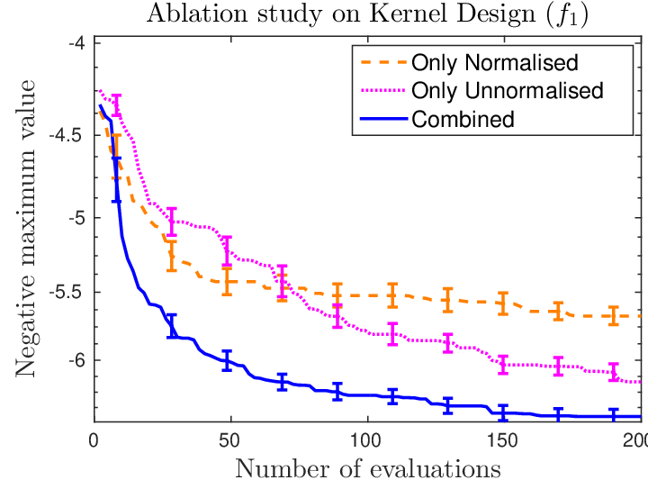
In Figure 7a, we compare NASBOT using only the normalised distance, only the unnormalised distance, and the combined kernel as in (7). While the individual distances performs well, the combined form outperforms both.
Next, we modify our EA procedure to optimise the acquisition. We execute NASBOT using only the EA modifiers which change the computational units (first four modifiers in Table 6), then using the modifiers which only change the structure of the networks (bottom 5 in Table 6), and finally using all 9 modifiers, as used in all our experiments. The combined version outperforms the first two.
Finally, we experiment with different choices for and in (7). As the figures indicate, the performance was not particularly sensitive to these choices.
Below we describe the three synthetic functions used in our synthetic experiments. applies for CNNs while apply for MLPs. Here denotes the average mass per layer, is the average in degree the layers, is the average out degree, is the shortest distance from to , is the average stride in CNNS, is the fraction of layers that are conv3, is the fraction of layers that are sigmoidal.


Appendix D Additional Discussion on Related Work
Historically, evolutionary (genetic) algorithms (EA) have been the most common method used for designing architectures [30, 21, 8, 51, 26, 36, 41]. EA techniques are popular as they provide a simple mechanism to explore the space of architectures by making a sequence of changes to networks that have already been evaluated. However, as we will discuss later, EA algorithms, while conceptually and computationally simple, are typically not best suited for optimising functions that are expensive to evaluate. A related line of work first sets up a search space for architectures via incremental modifications, and then explores this space via random exploration, MCTS, or A* search [25, 32, 6]. Some of the methods above can only optimise among feed forward structures, e.g. Fig. 1a, but cannot handle spaces with arbitrarily structured networks, e.g. Figs. 1b, 1c.
The most successful recent architecture search methods that can handle arbitrary structures have adopted reinforcement learning (RL) [1, 53, 54, 52]. However, architecture search is in essence an optimisation problem – find the network with the highest function value. There is no explicit need to maintain a notion of state and solve the credit assignment problem in RL [43]. Since RL is fundamentally more difficult than optimisation [16], these methods typically need to try a very large number of architectures to find the optimum. This is not desirable, especially in computationally constrained settings.